One-dimensional aggregation equation after blow up: existence, uniqueness and numerical simulation

Abstract

The nonlocal nonlinear aggregation equation in one space dimension is investigated. In the so-called attractive case smooth solutions blow up in finite time, so that weak measure solutions are introduced. The velocity involved in the equation becomes discontinuous, and a particular care has to be paid to its definition as well as the formulation of the corresponding flux. When this is done, the notion of duality solutions allows to obtain global in time existence and uniqueness for measure solutions. An upwind finite volume scheme is also analyzed, and the convergence towards the unique solution is proved. Numerical examples show the dynamics of the solutions after the blow up time.

2010 AMS subject classifications: Primary: 35B40, 35D30, 35L60, 35Q92; Secondary: 49K20.

Keywords: Aggregation equation, Weak measure solutions, Transport equation, Blow up, Finite volume scheme.

1 Introduction

This paper presents a survey of several results obtained by the authors concerning existence, uniqueness and numerical simulation of measure solutions for the one-dimensional aggregation equation in the attractive case. This equation describes aggregation phenomena in a population of individuals interacting under a continuous potential $W\,:\,\mathbb{R}\to\mathbb{R}$. If $\rho$ denotes the density of individuals, its dynamics is modelled by a nonlocal nonlinear conservation equation

$$\partial_{t}\rho+\partial_{x}\big{(}a(\partial_{x}W*\rho)\rho\big{)}=0,\qquad t>0,\quad x\in\mathbb{R}.$$ (1.1)

This equation is complemented with the initial condition $\rho(0,x)=\rho^{ini}$. Here $a\,:\,\mathbb{R}\to\mathbb{R}$ is a smooth given function which depends on the actual model under consideration. This model appears in many applications in physics and population dynamics. It is used for instance in the framework of granular media [2], in the description of crowd motion [11, 25], and in the description of the collective motion of cells or bacteria [27, 13, 14, 19], and the references therein. In many of these examples, the potential $W$ has a singularity at the origin. Due to this weak regularity, finite time blow up of regular solutions occurs and has caught the attention of several authors [24, 5, 3]. The context of weak measure solution is natural here, because of this blow up property as well as the conservative structure of the aggregation equation (1.1), which gives rise to a bound on the mass of measure solutions.

In this paper, we focus on these singular attractive potentials, sometimes called mild singular. More precisely, we introduce the following notion.

Definition 1.1 (pointy potential)

The interaction potential $W$ is said to be an attractive pointy potential if it satisfies the following assumptions:

$$\begin{array}[]{c}W\mbox{ is Lipschitz continuous, }W(x)=W(-x),\ W(0)=0,\\[5.69054pt] \mbox{ and }W\mbox{ is }\lambda\mbox{-concave for some }\lambda\geq 0,\mbox{ i.e. }W(x)-\frac{\lambda}{2}x^{2}\mbox{ is concave}.\end{array}$$ (1.2)

Depending upon the applications, the function $a$ may be linear ($a(x)=x$) or nonlinear. In what follows, we shall refer to the linear case when $a={\rm id}$ and the potential $W$ satisfies (1.2). In the nonlinear case additional assumptions have to be made. First, to obtain an attractive model, $a$ has to be nondecreasing. This is related to the so-called one-sided Lipschitz estimates, see Section 4 below for details. Therefore we consider the following set of assumptions on the velocity field:

$$a\in C^{1}(\mathbb{R}),\quad 0\leq a^{\prime}\leq\alpha,\quad\alpha>0.$$ (1.3)

Unfortunately, in this case, the class of admissible potentials has to be reduced, namely we are limited to potentials $W$ such that

$$\begin{array}[]{c}W\in C^{2}(\mathbb{R}\setminus\{0\})\mbox{ satisfies \eqref{hyp1} and there exists $w$ continuous, }\|w\|_{L^{1}(\mathbb{R})}=w_{0}\\[5.69054pt] \mbox{such that }W^{\prime\prime}=-\delta_{0}+w\mbox{ holds in the distributional sense}.\end{array}$$ (1.4)

The above assumptions include classical functions $W$ such as $W(x)=-|x|$ or $W(x)=e^{-|x|}-1$. As we shall see, each case deserves its own definition of the velocity.

Several authors have studied existence of global in time weak measure solution for the aggregation equation. In [9], global existence of weak measure solutions in the linear case, that is for $W$ satisfying (1.2), in $\mathbb{R}^{d}$ for any dimension $d\geq 1$ has been obtained using the gradient flow structure of this problem. In fact, for the aggregation equation in the case $a={\rm id}$, we can define the interaction energy by

$$\mathcal{W}(\rho)=\frac{1}{2}\int_{\mathbb{R}^{d}\times\mathbb{R}^{d}}W(x-y)\,\rho(dx)\rho(dy).$$

Then a gradient flow solution $\mu$ in the Wasserstein space is defined as a solution in the sense of distributions of the continuity equation

$$\partial_{t}\mu+\mathop{\rm div}\nolimits\big{(}v\mu\big{)}=0,\qquad v\in\partial^{0}\mathcal{W}(\mu),$$

where $\partial^{0}\mathcal{W}(\mu)$ denotes the element of minimal norm in $\partial\mathcal{W}(\mu)$, which is the subdifferential of $\mathcal{W}$ at the point $\mu$, see [1] for more details. Such a solution is constructed by performing the JKO scheme [22]. However this approach cannot be applied in the nonlinear case that is under assumptions (1.3)-(1.4) and there is, up to our knowledge, no numerical result based on this approach allowing to recover the dynamics of the solution after blow up.

An alternative strategy has been proposed by the authors, which consists in interpreting (1.1) as a conservative transport equation with velocity $a(\partial_{x}W*\rho)$. Since solutions blow up in finite time, eventually $\rho$ become measure-valued, and care has to be taken of the product $a(\partial_{x}W*\rho)\rho$: typically Dirac masses may appear and the velocity becomes discontinuous precisely at their location. Hence this requires the use of tools which have been developped for advection equations with discontinuous coefficients: pushforward by a generalized flow [29, 4], or duality solutions [6]. This paper will make use of the latter notion, which is recalled in the next Section. The first application to the aggregation equation was done in the particular case of chemotaxis in [19]. It has been extended later to more general aggregation equations in both the linear and nonlinear cases in [20]. The main drawback of this method is that it is presently limited to one space dimension. In the linear multidimensional case (as in [9]), the pushforward method has been successfully applied in [10]. We emphasize that in all cases the definition of the velocity and of its product with the measure $\rho$ has to be very carefully treated, as it is a key ingredient to prove the uniqueness of solutions.

Numerical simulations of solutions to (1.1) before the blow up time has been investigated in [8] with a finite volume method but no convergence result has been obtained, and in [12] thanks to a particle method. However, the dynamics of the solutions after the blow up time is not recovered in these works. Then, in [21], a finite volume scheme of Lax-Friedrichs type has been proposed and analyzed. This scheme has been designed in order to recover the dynamics of the solution after blow up time. In this paper, we study another finite volume scheme, based on an upwind approach. As in [21], the convergence of the scheme is proved and numerical simulations showing different blow up profiles are proposed.

The outline of the paper is the following. The next Section is devoted to the definition of duality solution to equation (1.1). We first recall useful results on duality solutions for transport equation. Then the definition of duality solution for the problem at hand is defined in subsection 2.2. A particular attention is given to the definition of the flux and velocity in both sets of assumptions. Section 3 is devoted to the proof of existence and uniqueness of weak measure solutions in the linear case ($a={\rm id}$ and $W$ satisfying (1.2)). The nonlinear case, that is assumptions (1.3)-(1.4), is studied in Section 4. Section 3 and 4 summarize the main results of the articles [19, 20]. Finally the numerical resolution of the problem is proposed in Section 5. The convergence of an upwind-type finite volume scheme is obtained in Theorem 5.4. Numerical illustrations showing different behaviours of solutions after blow up for different choices of the interaction potential are provided in subsection 5.4

2 Duality solutions

We will make use of the notations $C_{0}(\mathbb{R})$ for the set of continuous functions that vanish at infinity, $\mathcal{M}_{b}(\mathbb{R})$ for the space of finite measures on $\mathbb{R}$. For $\rho\in\mathcal{M}_{b}(\mathbb{R})$, its total mass is denoted $|\rho|(\mathbb{R})$. This space will be always endowed with the weak topology $\sigma(\mathcal{M}_{b},C_{0})$ and we denote $\mathcal{S}_{\mathcal{M}}:=C([0,T];{\mathcal{M}}_{b}(\mathbb{R})-\sigma({\mathcal{M}}_{b},C_{0}))$. Since we focus on scalar conservation laws, we can assume without loss of generality that the total mass of the system is scaled to $1$. Indeed, if the total mass is $M\neq 1$, then we rescale the density by introducing $\rho/M$, it suffices to change the definition of the function $a$ by introducing $\widetilde{a}(x)=a(Mx)$ which will always satisfies (1.3). Thus we will work in some space of probability measures, namely the Wasserstein space of order $q\geq 1$, which is the space of probability measures with finite order $q$ moment:

$$\mathcal{P}_{q}(\mathbb{R})=\left\{\mu\mbox{ nonnegative Borel measure},\mu(\mathbb{R})=1,\int|x|^{q}\mu(dx)<\infty\right\}.$$

2.1 Duality solutions for linear transport equation

We consider the conservative transport equation

$$\partial_{t}\rho+\partial_{x}\big{(}b(t,x)\rho\big{)}=0,\qquad(t,x)\in(0,T)\times\mathbb{R},$$ (2.5)

where $b$ is a given bounded Borel function. Since no regularity is assumed for $b$, solutions to (2.5) eventually are measures in space. A convenient tool to handle this is the notion of duality solutions, which are defined as weak solutions, the test functions being Lipschitz solutions to the backward linear transport equation

$$\displaystyle\partial_{t}p+b(t,x)\partial_{x}p=0,\qquad p(T,.)=p^{T}\in{\rm Lip}(\mathbb{R}).$$ (2.6)

In fact, a formal computation shows that $\frac{d}{dt}\left(\int_{\mathbb{R}}p(t,x)\rho(t,dx)\right)=0$, which defines the duality solutions for suitable $p$.

It is quite classical that a sufficient condition to ensure existence for (2.6) is that the velocity field be compressive, in the following sense:

Definition 2.1

We say that the function $b$ satisfies the one-sided Lipschitz (OSL) condition if

$$\partial_{x}b(t,.)\leq\beta(t)\qquad\mbox{for $\beta\in L^{1}(0,T)$, in the distributional sense}.$$ (2.7)

However, to have uniqueness, we need to restrict ourselves to reversible solutions of (2.6): let ${\mathcal{L}}$ denote the set of Lipschitz continuous solutions to (2.6), and define the set ${\mathcal{E}}$ of exceptional solutions by

$${\mathcal{E}}=\Big{\{}p\in{\mathcal{L}}\mbox{ such that }p^{T}\equiv 0\Big{\}}.$$

The possible loss of uniqueness corresponds to the case where ${\mathcal{E}}$ is not reduced to $\{\rho=0\}$.

Definition 2.2

We say that $p\in{\mathcal{L}}$ is a reversible solution to (2.6) if $p$ is locally constant on the set

$${\mathcal{V}}_{e}=\Big{\{}(t,x)\in[0,T]\times\mathbb{R};\ \exists\ p_{e}\in{\mathcal{E}},\ p_{e}(t,x)\not=0\Big{\}}.$$

We refer to [6] for complete statements of the characterization and properties of reversible solutions. Then, we can state the definition of duality solutions.

Definition 2.3

We say that $\rho\in\mathcal{S}_{\mathcal{M}}:=C([0,T];{\mathcal{M}}_{b}(\mathbb{R})-\sigma({\mathcal{M}}_{b},C_{0}))$ is a duality solution to (2.5) if for any $0<\tau\leq T$, and any reversible solution $p$ to (2.6) with compact support in $x$, the function $\displaystyle t\mapsto\int_{\mathbb{R}}p(t,x)\rho(t,dx)$ is constant on $[0,\tau]$.

We summarize now some useful properties of duality solutions.

Theorem 2.4

(Bouchut, James [6])

1. Given $\rho^{\circ}\in{\mathcal{M}}_{b}(\mathbb{R})$, under the assumptions (2.7), there exists a unique $\rho\in\mathcal{S}_{\mathcal{M}}$, duality solution to (2.5), such that $\rho(0,.)=\rho^{\circ}$.
   Moreover, if $\rho^{\circ}$ is nonnegative, then $\rho(t,\cdot)$ is nonnegative for a.e. $t\geq 0$. And we have the mass conservation

   $$|\rho(t,\cdot)|(\mathbb{R})=|\rho^{\circ}|(\mathbb{R}),\quad\mbox{ for a.e. }t\in]0,T[.$$

2. Backward flow and push-forward: the duality solution satisfies

   $$\forall\,t\in[0,T],\forall\,\phi\in C_{0}(\mathbb{R}),\quad\int_{\mathbb{R}}\phi(x)\rho(t,dx)=\int_{\mathbb{R}}\phi(X(t,0,x))\rho^{0}(dx),$$ (2.8)

   where the backward flow $X$ is defined as the unique reversible solution to

   $$\partial_{t}X+b(t,x)\partial_{x}X=0\quad\mbox{ in }]0,s[\times\mathbb{R},\qquad X(s,s,x)=x.$$

3. For any duality solution $\rho$, we define the generalized flux corresponding to $\rho$ by $b{\mbox{\tiny$\Delta$}}\rho=-\partial_{t}u$, where $u=\int^{x}\rho\,dx$.

   There exists a bounded Borel function $\widehat{b}$, called universal representative of $b$, such that $\widehat{b}=b$ almost everywhere, $b{\mbox{\tiny$\Delta$}}\rho=\widehat{b}\rho$ and for any duality solution $\rho$,

   $$\partial_{t}\rho+\partial_{x}(\widehat{b}\rho)=0\qquad\hbox{in the distributional sense.}$$

4. Stability: Let $(b_{n})$ be a bounded sequence in $L^{\infty}(]0,T[\times\mathbb{R})$, such that $b_{n}\rightharpoonup b$ in $L^{\infty}(]0,T[\times\mathbb{R})-w\star$. Assume $\partial_{x}b_{n}\leq\beta_{n}(t)$, where $(\beta_{n})$ is bounded in $L^{1}(]0,T[)$, $\partial_{x}b\leq\beta\in L^{1}(]0,T[)$. Consider a sequence $(\rho_{n})\in\mathcal{S}_{\mathcal{M}}$ of duality solutions to

   $$\partial_{t}\rho_{n}+\partial_{x}(b_{n}\rho_{n})=0\quad\hbox{in}\quad]0,T[\times\mathbb{R},$$

   such that $\rho_{n}(0,.)$ is bounded in ${\mathcal{M}}_{b}(\mathbb{R})$, and $\rho_{n}(0,.)\rightharpoonup\rho^{\circ}\in{\mathcal{M}}_{b}(\mathbb{R})$.

   Then $\rho_{n}\rightharpoonup\rho$ in $\mathcal{S}_{\mathcal{M}}$, where $\rho\in\mathcal{S}_{\mathcal{M}}$ is the duality solution to

   $$\partial_{t}\rho+\partial_{x}(b\rho)=0\quad\hbox{in}\quad]0,T[\times\mathbb{R},\qquad\rho(0,.)=\rho^{\circ}.$$

   Moreover, $\widehat{b}_{n}\rho_{n}\rightharpoonup\widehat{b}\rho$ weakly in ${\mathcal{M}}_{b}(]0,T[\times\mathbb{R})$.

The set of duality solutions is clearly a vector space, but it has to be noted that a duality solution is not a priori defined as a solution in the sense of distributions. However, assuming that the coefficient $b$ is piecewise continuous, we have the following equivalence result:

Theorem 2.5

(Bouchut, James [6]) Let us assume that in addition to the OSL condition (2.7), $b$ is piecewise continuous on $]0,T[\times\mathbb{R}$ where the set of discontinuity is locally finite. Then there exists a function $\widehat{b}$ which coincides with $b$ on the set of continuity of $b$.

With this $\widehat{b}$, $\rho\in\mathcal{S}_{\mathcal{M}}$ is a duality solution to (2.5) if and only if $\partial_{t}\rho+\partial_{x}(\widehat{b}\rho)=0$ in ${\mathcal{D}}^{\prime}(\mathbb{R})$. Then the generalized flux $b{\mbox{\tiny$\Delta$}}\rho=\widehat{b}\rho$. In particular, $\widehat{b}$ is a universal representative of $b$.

This result comes from the uniqueness of solutions to the Cauchy problem for both kinds of solutions, see [6, Theorem 4.3.7].

2.2 Aggregation equation as a transport equation

Equipped with this notion of solutions, we can now define duality solutions for the aggregation equation. The idea was introduced in [7] in the context of pressureless gases. It was next applied to chemotaxis in [19] and generalized in [20].

Definition 2.6

We say that $\rho\in\mathcal{S}_{\mathcal{M}}$ is a duality solution to (1.1) if there exists $\widehat{a}_{\rho}\in L^{\infty}((0,T)\times\mathbb{R})$ and $\beta\in L^{1}_{loc}(0,T)$ satisfying $\partial_{x}\widehat{a}_{\rho}\leq\beta$ in ${\mathcal{D}}^{\prime}((0,T)\times\mathbb{R})$, such that for all $0<t_{1}<t_{2}<T$,

$$\partial_{t}\rho+\partial_{x}(\widehat{a}_{\rho}\rho)=0$$ (2.9)

in the sense of duality on $(t_{1},t_{2})$, and $\widehat{a}_{\rho}=a(W^{\prime}*\rho)$ a.e. We emphasize that it means that the final datum for (2.6) should be at $t_{2}$ instead of $T$.

This allows at first to give a meaning to the notion of distributional solutions, but it turns out that uniqueness is a crucial issue. For that, a key point is a specific definition of the product $\widehat{a}_{\rho}\rho$, which can be seen as the flux of the system. Indeed, when concentrations occur in conservation equations, measure-valued solutions can have Dirac deltas, which makes the velocity a BV function. A key point for the definition of the flux is to be able to handle products of BV functions with measure-valued functions. In the framework of the aggregation equation, a definition of the flux can be obtained using the dependancy of the velocity on the solution. Let us make this point precise in both situations considered in this paper.

In the linear case that is $a={\rm id}$ and $W$ satisfying assumptions (1.2), the flux is defined by

$$J=\widehat{a}_{\rho}\rho,\qquad\widehat{a}_{\rho}(t,x):=\partial^{0}W*\rho(t,x)=\int_{x\neq y}W^{\prime}(x-y)\rho(t,dy).$$ (2.10)

This definition is motivated by the following stability result:

Lemma 2.7

[10, Lemma 3.1] Let us assume that $W$ satisfies (1.2). Let $(W_{n})_{n\in\mathbb{N}^{*}}$ be a sequence in $C^{1}(\mathbb{R})$ satisfying (1.2) with the same constant $\lambda$ not depending on $n$ and such that

$$sup_{x\in\mathbb{R}\setminus(-\frac{1}{n},\frac{1}{n})}\big{|}W^{\prime}_{n}(x)-W^{\prime}(x)\big{|}\leq\frac{1}{n},\qquad\mbox{ for all }n\in\mathbb{N}^{*}.$$

If the sequence $\rho_{n}\rightharpoonup\rho$ weakly as measures, then for every continuous compactly supported $\phi$, we have

$$\lim_{n\to+\infty}\iint_{\mathbb{R}\times\mathbb{R}}\phi(x)W^{\prime}_{n}(x-y)\rho_{n}(dx)\rho_{n}(dy)=\iint_{\mathbb{R}\times\mathbb{R}\setminus D}\phi(x)W^{\prime}(x-y)\rho(dx)\rho(dy),$$

where $D$ is the diagonal of $\mathbb{R}\times\mathbb{R}$: $D=\{(x,x),\,x\in\mathbb{R}\}$.

In the nonlinear case given by assumptions (1.3) and (1.4), we use the assumption on $W$ to obtain a definition of the flux. Indeed we can formally take the convolution of (1.4) by $\rho$, then multiply by $a(W^{\prime}*\rho)$. Denoting by $A$ the antiderivative of $a$ such that $A(0)=0$ and using the chain rule we obtain formally

$$-\partial_{x}(A(W^{\prime}*\rho))=-a(W^{\prime}*\rho)W^{\prime\prime}*\rho=a(W^{\prime}*\rho)(\rho-w*\rho).$$ (2.11)

Thus a natural formulation for the flux $J$ is given by

$$J:=-\partial_{x}\big{(}A(W^{\prime}*\rho)\big{)}+a(W^{\prime}*\rho)w*\rho.$$ (2.12)

The product $a(W^{\prime}*\rho)w*\rho$ is well defined since $w*\rho$ is Lipschitz. The function $A(W^{\prime}*\rho)$ is a $BV(\mathbb{R})$ function. Then $J$ is defined in the sense of measures. The analogue of the stability result of Lemma 2.7 is verified since if $\rho_{n}\rightharpoonup\rho$, we have that $W^{\prime}*\rho_{n}\rightharpoonup W*\rho$ a.e., which induces that in the sense of distributions $J_{n}$ converges to $J$. Moreover, from the chain rule for BV functions (or Vol’pert calculus), there exists a function $\widehat{a}_{\rho}$ such that $\widehat{a}_{\rho}=a(W^{\prime}*\rho)$ a.e., and $J=\widehat{a}_{\rho}\rho$. Then it can be verified (see Section 3.3 in [20]) that in the case $a={\rm id}$, $\widehat{a}_{\rho}$ is given by (2.10).

This idea of definition of the flux comes from [19], where the particular case $W(x)=\frac{1}{2}e^{-|x|}-\frac{1}{2}$ appearing in chemotaxis has been treated. An analogous situation arising in plasma physics is considered in [18]. In a similar context, other definitions of the product can be found, see [26] in the one-dimensional setting, and [28] for a generalization in two space dimensions, where defect measures are used. In this latter work, more singular potentials are considered, but the uniqueness of the weak measure solution is not recovered.

3 Existence and uniqueness in the linear case

In this section we state and prove the existence and uniqueness theorem for duality solutions to the aggregation equation (1.1) in the linear case, that is $a={\rm id}$ and a general pointy potential $W$ satisfying (1.2).

Theorem 3.1

[20, Theorem 3.7] Let $W$ as in (1.2) and $a=\mbox{\rm id}$. Assume that $\rho^{ini}\in\mathcal{P}_{1}(\mathbb{R})$. Then for any $T>0$, there exists a unique $\rho\in\mathcal{S}_{\mathcal{M}}$ such that $\rho(0)=\rho^{ini}$, $\rho(t)\in\mathcal{P}_{1}(\mathbb{R})$ for any $t\in(0,T)$, and $\rho$ is a duality solution to equation (1.1) with universal representative $\widehat{a}_{\rho}$ in (2.9) defined in (2.10). Moreover we have $\rho=X_{\#}\rho^{ini}$ where $X$ is the backward flow corresponding to $\widehat{a}_{\rho}$.

The proof of this result is splitted into several steps corresponding to the following subsections.

Remark 3.2

This result has been extended to any dimension $d\geq 1$ in [10] and it has been proved that such solutions are equivalent to gradient flow solutions obtained in [9].

3.1 One-sided Lipschitz estimate

Lemma 3.3

Let $\rho(t)\in\mathcal{M}_{b}(\mathbb{R})$ be nonnegative for all $t\geq 0$. Then under assumptions (1.2) the function $(t,x)\mapsto\widehat{a}_{\rho}(t,x)$ defined in (2.10) satisfies the one-sided Lipschitz estimate

$$\widehat{a}_{\rho}(t,x)-\widehat{a}_{\rho}(t,y)\leq\lambda(x-y)|\rho|(\mathbb{R}),\quad\mbox{ for all }\ x>y,\ t\geq 0$$

Proof.

Using assumption (1.2), $x\mapsto W^{\prime}(x)-\lambda x$ is a nonincreasing function on $\mathbb{R}\setminus\{0\}$. Therefore $\lim_{x\to 0^{\pm}}W^{\prime}(x)=W^{\prime}(0^{\pm})$ exists and from the oddness of $W^{\prime}$, we deduce that $W^{\prime}(0^{-})=-W^{\prime}(0^{+})$. Moreover, for all $x>y$ in $\mathbb{R}\setminus\{0\}$ we have $W^{\prime}(x)-\lambda x\leq W^{\prime}(y)-\lambda y$. Thus we have the one-sided Lipschitz estimate (OSL) for $W^{\prime}$

$$\forall\,x>y\in\mathbb{R}\setminus\{0\},\qquad W^{\prime}(x)-W^{\prime}(y)\leq\lambda(x-y).$$ (3.13)

Letting $y\to 0^{\pm}$ we deduce that for all $x>0$, $W^{\prime}(x)-\lambda x\leq W^{\prime}(0^{+})$ and $W^{\prime}(x)-\lambda x\leq W^{\prime}(0^{-})$. Thus we also have the one-sided estimate

$$W^{\prime}(x)\leq\lambda x,\quad\mbox{ for all }x>0.$$ (3.14)

By definition of $\widehat{a}_{\rho}$ (2.10), we have

$$\widehat{a}_{\rho}(x)-\widehat{a}_{\rho}(y)=\int_{z\neq x,z\neq y}(W^{\prime}(x-z)-W^{\prime}(y-z))\rho(dz)+W^{\prime}(x-y)\int_{z\in\{x\}\cup\{y\}}\rho(dz),$$

where we use the oddness of $W^{\prime}$ (1.2) in the last term. Let us assume that $x>y$, from (3.13), we deduce that $W^{\prime}(x-z)-W^{\prime}(y-z)\leq\lambda(x-y)$ and with (3.14), we deduce $W^{\prime}(x-y)\leq\lambda(x-y)$. Thus, using the nonnegativity of $\rho$, we deduce the one-sided Lipschitz (OSL) estimate for $\widehat{a}_{\rho}$.

3.2 Dynamics of aggregates

We first assume that the initial density is given by a finite sum of Dirac deltas: $\rho^{ini}_{n}=\sum_{i=1}^{n}m_{i}\delta_{x_{i}^{0}}$ where $x_{1}^{0}<x_{2}^{0}<\dots<x_{n}^{0}$ and the $m_{i}$-s are nonnegative. Moreover, we assume that $\sum_{i=1}^{n}m_{i}=1$ and that the first moment $\sum_{i=1}^{n}m_{i}|x_{i}^{0}|$ is uniformly bounded with respect to $n$, so that $\rho^{ini}_{n}\in\mathcal{P}_{1}(\mathbb{R})$. We look for a solution in the form $\rho_{n}(t,x)=\sum_{i=1}^{n}m_{i}\delta_{x_{i}(t)}$. Injecting this expression into the definition of the macroscopic velocity in (2.10), we get

$$\widehat{a}_{\rho_{n}}(x)=\left\{\begin{array}[]{ll}\displaystyle\sum_{j\neq i}m_{j}W^{\prime}(x_{i}-x_{j})&\displaystyle\qquad\mbox{ if }x=x_{i},\ i=1,\ldots,n\\[5.69054pt] \displaystyle\sum_{j=1}^{n}m_{j}W^{\prime}(x-x_{j})&\displaystyle\qquad\mbox{ otherwise}.\end{array}\right.$$ (3.15)

We emphasize that this macroscopic velocity is defined everywhere, which allows to give a sense to its product with the measure $\rho_{n}$. Then, $\rho_{n}$ is a solution in the sense of distributions of (2.9) provided the sequence $(x_{i})_{i=1,\ldots,n}$ satisfies the ODE system

$$x^{\prime}_{i}(t)=\sum_{j\neq i}m_{j}W^{\prime}(x_{i}-x_{j}),\qquad x_{i}(0)=x_{i}^{0},\qquad i=1,\ldots,n_{\ell},$$ (3.16)

where $n_{\ell}\leq n$ is the number of distinct particles, i.e. $n_{\ell}=\#\{i\in\{1,\ldots,N\},x_{i}\neq x_{j},\forall\,j\}$. Then we define the dynamics of aggregates by:

• When the $x_{i}$ are all distinct, they are solutions of system (3.16) (with zero right hand side if $n_{\ell}=1$).

• When two particles collide, they stick to form a bigger particle whose mass is the sum of both particles and the dynamics continues with one particle less.

Clearly this choice of the dynamics implies mass conservation. It also preserves the one-sided Lipschitz estimate for the velocity. Finally, setting $\rho_{n}(t,x)=\sum_{i=1}^{n_{\ell}}m_{i}\delta_{x_{i}(t)}(x)$, the sticky particle dynamics defines a distributional solution to (2.9). Hence, we are in position to apply Theorem 2.5, and deduce that $\rho_{n}(t,x)$ is a duality solution for given initial data $\rho_{n}^{ini}$.

For a general initial datum $\rho^{ini}$ in $\mathcal{P}_{1}(\mathbb{R})$, we approximate it by a sequence of measures $\rho^{ini}_{n}$, for which we can construct a duality solution as above. Then we use the stability of duality solutions (see Theorem 2.4) to pass to the limit in the approximation. This allows to prove the existence result in Theorem 3.1.

3.3 Contraction property

Uniqueness in Theorem 3.1 is obtained thanks to a contraction argument in the Wasserstein distance. In the present one dimensional framework, the definition of the Wasserstein distance can be simplified using the generalized inverse. More precisely, let $\rho$ be a nonnegative measure, we denote by $F$ its cumulative distribution function. Then we can define the generalized inverse of $F$ (or monotone rearrangement of $\rho$) by $F^{-1}(z):=\inf\{x\in\mathbb{R}/F(x)>z\}$, it is a right-continuous and nondecreasing function as well, defined on $[0,1]$. We have for every nonnegative Borel map $\xi$,

$$\int_{\mathbb{R}}\xi(x)\rho(dx)=\int_{0}^{1}\xi(F^{-1}(z))\,dz.$$

In particular, $\rho\in\mathcal{P}_{1}(\mathbb{R})$ if and only if $F^{-1}\in L^{1}(0,1)$. Then, if $\rho_{1}$ and $\rho_{2}$ belong to $\mathcal{P}_{1}(\mathbb{R})$, with monotone rearrangement $F_{1}$ and $F_{2}$, respectively, we have the explicit expression of the Wasserstein distance (see [30])

$$d_{W1}(\rho_{1},\rho_{2})=\int_{0}^{1}|F_{1}(z)-F_{2}(z)|\,dz.$$ (3.17)

Let $\rho$ be a duality solution that satisfies (2.9) in the distributional sense. Denoting $F$ its cumulative distribution function and $F^{-1}$ its generalized inverse, we have by integration of (2.9)

$$\partial_{t}F+\widehat{a}_{\rho}\partial_{x}F=0,$$

so that the generalized inverse is a solution to

$$\partial_{t}F^{-1}(t,z)=\widehat{a}_{\rho}(t,F^{-1}(z)).$$ (3.18)

Moreover thanks to a change of variables in (2.10),

$$\widehat{a}_{\rho}(t,F^{-1}(z))=\int_{y\neq z}W^{\prime}\big{(}F^{-1}(z)-F^{-1}(y)\big{)}\,dy.$$

Now using (3.18) and since $W^{\prime}$ is one-sided Lipschitz continuous (3.13), we obtain the following contraction property, which implies uniqueness.

Proposition 3.4

Assume $\rho_{1}(t,\cdot),\rho_{2}(t,\cdot)\in\mathcal{P}_{1}(\mathbb{R})$ satisfy (2.9) in the sense of distributions, with $\widehat{a}_{\rho_{i}}$ given by (2.10), and initial data $\rho_{1}^{ini}$ and $\rho_{2}^{ini}$. Then we have, for all $t>0$

$$d_{W1}(\rho_{1}(t,\cdot),\rho_{2}(t,\cdot))\leq e^{2\lambda t}d_{W1}(\rho_{1}^{ini},\rho_{2}^{ini}).$$

4 Existence and uniqueness in the nonlinear case

In this Section, we focus on the nonlinear case characterized by assumptions (1.3) and (1.4). The main result is the following theorem, which includes the existence result of [19], where the particular case $W(x)=\frac{1}{2}e^{-|x|}-\frac{1}{2}$ arising in chemotaxis has been considered, and the existence result presented in [18], when $W(x)=-|x|/2$, which appears in many applications in physics or biology.

Theorem 4.1

[20, Theorem 3.10] Let be given $\rho^{ini}\in\mathcal{P}_{1}(\mathbb{R})$. Let us assume that $a$ and $W$ are such as in (1.4). For all $T>0$ there exists a unique duality solution $\rho$ of (1.1) in the sense of Definition 2.6 that satisfies in the distributional sense

$$\partial_{t}\rho+\partial_{x}J=0,$$ (4.19)

where $J$ is defined by (2.12). Moreover, $\rho(t)\in\mathcal{P}_{1}(\mathbb{R})$ for $t\in(0,T)$.

The proof follows the same steps as the preceding one, except that uniqueness here relies on an entropy estimate. In this respect, we emphasize now some links with entropy solutions of scalar conservation laws.

Remark 4.2

If $w=0$ in (1.4), then $\rho$ is the unique duality solution of Theorem 4.1 if and only if $u=W^{\prime}*\rho$ is an entropy solution to $\partial_{t}u+\partial_{x}A(u)=0$. (see [20, Theorem 5.7])

4.1 One sided-Lipschitz estimate

Lemma 4.3

Assume $0\leq\rho\in{\mathcal{M}}_{b}(\mathbb{R})$ and that (1.4) is satisfied. Then the function $x\mapsto a(W^{\prime}*\rho)$ satisfies the OSL condition (2.7).

Proof.

Using the assumption on $W$ in (1.4), we deduce that

$$\partial_{xx}W*\rho=-\rho+w*\rho.$$

Therefore,

$$\partial_{x}(a(\partial_{x}W*\rho))=a^{\prime}(\partial_{x}W*\rho)(-\rho+w*\rho)\leq a^{\prime}(\partial_{x}W*\rho)w*\rho,$$

where we use the nonnegativity of $\rho$ in the last inequality. Then from assumption (1.3) on the function $a$ we get

$$\partial_{x}(a(\partial_{x}W*\rho))\leq\alpha\|\rho\|_{L^{1}}\|w\|_{L^{\infty}}.$$

4.2 Dynamics of aggregates

Following the idea in subsection 3.2, we first approximate the initial data $\rho^{ini}$ by a finite sum of Dirac deltas: $\rho^{ini}_{n}=\sum_{i=1}^{n}m_{i}\delta_{x_{i}^{0}}$ where $x_{1}^{0}<x_{2}^{0}<\dots<x_{n}^{0}$ and the $m_{i}$ are nonnegative. We assume that $\sum_{i=1}^{n}m_{i}=1$ and $\sum_{i=1}^{n}m_{i}|x_{i}^{0}|$ is uniformly bounded with respect to $n$, i.e. $\rho^{ini}_{n}\in\mathcal{P}_{1}(\mathbb{R})$. We look for a sequence $(\rho_{n})_{n}$ solving in the distributional sense $\partial_{t}\rho_{n}+\partial_{x}J_{n}=0$ where the flux $J_{n}$ is given by (2.12). Let $\rho_{n}(t,x)=\sum_{i=1}^{n}m_{i}\delta_{x_{i}(t)}$. From assumption (1.4) on $W$, we deduce that

$$W^{\prime}(x)=-H(x)+\widetilde{w}(x),\quad\mbox{ where }\widetilde{w}(x)=\int^{x}_{0}w(y)\,dy+\frac{1}{2}.$$

Then, we have

$$W^{\prime}*\rho_{n}(x_{i}^{+})=-\sum_{j=1}^{i}m_{j}+\sum_{j=1}^{n}m_{j}\widetilde{w}(x_{i}-x_{j});\quad W^{\prime}*\rho_{n}(x_{i}^{-})=m_{i}+W^{\prime}*\rho_{n}(x_{i}^{+}),$$

where we use the standard notation $f(x_{i}^{+})=\lim_{x\underset{>}{\to}x_{i}}f(x)$ and $f(x_{i}^{-})=\lim_{x\underset{<}{\to}x_{i}}f(x)$. From these identities, we deduce that in the distributional sense

$$\partial_{x}\big{(}A(W^{\prime}*\rho_{n})\big{)}=a(W^{\prime}*\rho_{n})w*\rho_{n}+\sum_{i=1}^{n}[A(W^{\prime}*\rho_{n})]_{x_{i}}\delta_{x_{i}},$$

where $[f]_{x_{i}}=f(x_{i}^{+})-f(x_{i}^{-})$ is the jump of the function $f$ at $x_{i}$. Then we find that $\rho_{n}$ satisfies (4.19) in the sense of distributions if we have

$$m_{i}x^{\prime}_{i}(t)=-[A(W^{\prime}*\rho_{n})]_{x_{i}(t)},\quad\mbox{ for }i=1,\dots,n_{\ell}.$$ (4.20)

This system of ODEs is complemented by the initial data $x_{i}(0)=x_{i}^{0}$.

Then the dynamics of aggregates is given as in subsection 3.2 by (4.20) as long as particles are all distinct, and by a sticky dynamics at collisions. By construction, $\rho_{n}(t,x)=\sum_{i=1}^{n_{\ell}}m_{i}\delta_{x_{i}(t)}(x)$ is a duality solution as in Theorem 4.1 for given initial data $\rho_{n}^{ini}$.

For a general initial datum $\rho^{ini}$ in $\mathcal{P}_{1}(\mathbb{R})$, we approximate it by a sequence of measures $\rho^{ini}_{n}$, for which we can construct a duality solution as above. Then we use the stability of duality solutions (see Theorem 2.4) to pass to the limit in the approximation.

4.3 Uniqueness

The strategy used in subsection 3.3 cannot be used here, since it strongly relies on the linearity of $a$. Then we use an analogy with entropy solutions for scalar conservation laws. Indeed, the quantity $W^{\prime}*\rho$ solves a scalar conservation law with source term, for which we can prove the following entropy estimate:

Proposition 4.4

[19, Lemma 4.5] Let us assume that assumptions (1.4) hold. For $T>0$, let $\rho\in C([0,T],\mathcal{P}_{1}(\mathbb{R}))$ satisfy (2.12)-(4.19) in the sense of distributions. Then $u:=W^{\prime}*\rho$ is a weak solution of

$$\partial_{t}u+\partial_{x}A(u)=a(u)w*\rho+\partial_{x}(w*A(u))-w*(a(u)w*\rho).$$ (4.21)

Moreover, if we assume that the entropy condition

$$\partial_{x}u\leq w*\rho$$ (4.22)

holds, then for any twice continuously differentiable convex function $\eta$, we have

$$\partial_{t}\eta(u)+\partial_{x}q(u)-\eta^{\prime}(u)a(u)w*\rho+\eta^{\prime}(u)\big{(}\partial_{x}(w*A(u))-w*(a(u)w*\rho))\leq 0,$$ (4.23)

where $q$, the entropy flux, is given by $\displaystyle q(x)=\int_{0}^{x}\eta^{\prime}(y)a(y)\,dy$.

This entropy estimate allows to deal with uniqueness. Consider two solutions $\rho_{1}$ and $\rho_{2}$ with initial data $\rho_{1}^{ini}$ and $\rho_{2}^{ini}$, as in Theorem 4.1. Since $\rho_{1}$ and $\rho_{2}$ are nonnegative, we deduce from (1.4) that both $u_{1}:=W^{\prime}*\rho_{1}$ and $u_{2}=W^{\prime}*\rho_{2}$ satisfy (4.22). Starting from the entropy inequality (4.23) with the family of Kružkov entropies $\eta_{\kappa}(u)=|u-\kappa|$ and using the doubling of variable technique developed by Kružkov, we show

$$\begin{array}[]{ll}\displaystyle\frac{d}{dt}\int_{\mathbb{R}}\big{|}u_{1}-u_{2}\big{|}\leq&\|w\|_{Lip}\int_{\mathbb{R}}\big{|}A(u_{1})-A(u_{2})\big{|}\,dx\\ &\displaystyle+\big{(}1+\|w\|_{\infty}\big{)}\int_{\mathbb{R}}\big{|}a(u_{1})w*\rho_{1}-a(u_{2})w*\rho_{2}\big{|}\,dx.\end{array}$$

From (1.3) and the bound on $\rho(t)$ in $\mathcal{P}_{1}(\mathbb{R})$ for all $t$, we deduce that $u_{i}$, $i=1,2$ are bounded in $L^{\infty}_{t,x}$. Then we get

$$\frac{d}{dt}\int_{\mathbb{R}}\big{|}u_{1}-u_{2}\big{|}\leq C\Big{(}\int_{\mathbb{R}}\big{|}u_{1}-u_{2}\big{|}\,dx+\int_{\mathbb{R}}\big{|}w*\rho_{1}-w*\rho_{2}\big{|}\,dx\Big{)},$$ (4.24)

where we use once again assumption on $a$ in (1.3). Taking the convolution with $w$ of equation (4.19) we deduce

$$\partial_{t}w*\rho_{i}-\partial_{x}\big{(}w*A(u_{i})\big{)}+w*\big{(}a(u_{i})w*\rho_{i}\big{)}=0,\qquad i=1,2.$$

We deduce from (1.3) and the Lipschitz bound on $w$ that

$$\frac{d}{dt}\int_{\mathbb{R}}\big{|}w*\rho_{1}-w*\rho_{2}\big{|}\leq C\Big{(}\int_{\mathbb{R}}\big{|}u_{1}-u_{2}\big{|}\,dx+\int_{\mathbb{R}}\big{|}w*\rho_{1}-w*\rho_{2}\big{|}\,dx\Big{)}.$$ (4.25)

Summing (4.24) and (4.25), we deduce applying a Gronwall lemma that for all $T>0$ there exists a nonnegative constant $C_{T}$ such that for all $t\in[0,T]$,

$$\begin{array}[]{l}\displaystyle\int_{\mathbb{R}}\Big{(}\big{|}W^{\prime}*\rho_{1}-W^{\prime}*\rho_{2}\big{|}(t)+\big{|}w*\rho_{1}-w*\rho_{2}\big{|}(t)\Big{)}\,dx\\ \displaystyle\leq C_{T}\int_{\mathbb{R}}\Big{(}\big{|}W^{\prime}*\rho_{1}^{ini}-W^{\prime}*\rho_{2}^{ini}\big{|}+\big{|}w*\rho_{1}^{ini}-w*\rho_{2}^{ini}\big{|}\Big{)}\,dx.\end{array}$$

The uniqueness follows easily.

5 Numerical simulations

An important advantage of the approach presented in this paper, is that it allows to prove convergence of well designed finite volume schemes. Numerical simulations of duality solutions for linear scalar conservation laws with discontinuous coefficients have been proposed and analyzed in [16]. In the present nonlinear context, a careful discretization of the velocity has to be implemented in order to recover the dynamics of aggregates after blow up time. In [21] a finite volume scheme of Lax-Friedrichs type is proposed and analyzed. Up to our knowledge, this is the only example of numerical scheme allowing to recover the dynamics of measure solutions after blow up. In this paper, we perform the same analysis on an upwind-type scheme, which is less diffusive than the Lax-Friedrichs scheme of [21]. Numerical simulations are also proposed.

5.1 Upwind finite volume scheme

Let us consider a mesh with constant space step $\Delta x$, and denote $x_{i}=i\Delta x$ for $i\in\mathbb{Z}$. We fix a constant time step $\Delta t$, and set $t_{n}=n\Delta t$ for $n\in\mathbb{N}$. For a given nonnegative measure $\rho^{ini}\in\mathcal{P}_{1}(\mathbb{R})$, we define for $i\in\mathbb{Z}$,

$$\rho_{i}^{0}=\frac{1}{\Delta x}\int_{C_{i}}\rho^{ini}(dx)\geq 0.$$ (5.26)

Since $\rho^{ini}$ is a probability measure, the total mass of the system is $\sum_{i}\Delta x\rho_{i}^{0}=1$. Assuming that an approximating sequence $(\rho_{i}^{n})_{i\in\mathbb{Z}}$ is known at time $t_{n}$, we compute the approximation at time $t_{n+1}$ by:

$$\rho_{i}^{n+1}=\rho_{i}^{n}-\frac{\Delta t}{\Delta x}\big{(}({a}^{n}_{i})_{+}\rho_{i}^{n}+({a}^{n}_{i+1})_{-}\rho_{i+1}^{n}-({a}^{n}_{i-1})_{+}\rho_{i-1}^{n}-({a}^{n}_{i})_{-}\rho_{i}^{n}\big{)}$$ (5.27)

The notation $(a)_{+}=\max\{0,a\}$ stands for the positive part of the real $a$ and respectively $(a)_{-}=\min\{0,a\}$ for the negative part. Then we define the flux by

$$J_{i+1/2}^{n}=({a}^{n}_{i})_{+}\rho_{i}^{n}+({a}^{n}_{i+1})_{-}\rho_{i+1}^{n}$$ (5.28)

A key point is the definition of the discrete velocity which should be done in accordance with (2.10) in the linear case and with (2.12) in the nonlinear case.

In the linear case, the discretization of the velocity is given by

$$a_{i}^{n}=\widehat{a}(t_{n},x_{i})=\sum_{j\neq i}W^{\prime}(x_{i}-x_{j})\rho_{j}^{n}\Delta x.$$ (5.29)

In the nonlinear case, we define

$$a_{i}^{n}=\left\{\begin{array}[]{ll}a(\partial_{x}S_{i+1/2}),&\mbox{ if }\ \partial_{x}S_{i+1/2}^{n}=\partial_{x}S_{i-1/2}^{n},\\[5.69054pt] \displaystyle\frac{A(\partial_{x}S_{i+1/2}^{n})-A(\partial_{x}S_{i-1/2}^{n})}{\partial_{x}S_{i+1/2}^{n}-\partial_{x}S_{i-1/2}^{n}},&\mbox{ otherwise.}\end{array}\right.$$ (5.30)

In this definition we have set $S_{i}^{n}$ an approximation of $W*\rho(t_{n},x_{i})$. Using (1.4), $S_{i}^{n}$ is a solution to

$$-\frac{\partial_{x}S_{i+1/2}^{n}-\partial_{x}S_{i-1/2}^{n}}{\Delta x}+\nu_{i}^{n}=\rho_{i}^{n},\qquad\partial_{x}S_{i+1/2}^{n}=\frac{S_{i+1}^{n}-S_{i}^{n}}{\Delta x}.$$ (5.31)

The quantity $(\nu_{i}^{n})_{i}$ corresponds to an approximation of $(w*\rho(t_{n},x_{i}))_{i}$. We will use the following discretization

$$\nu_{i}^{n}=\sum_{k\in\mathbb{Z}}\rho_{k}^{n}w_{ki}\Delta x,\quad\mbox{ with }\quad\frac{1}{2}(w_{ki}+w_{ki+1})=\frac{1}{\Delta x}\int_{x_{i}}^{x_{i+1}}w(x-x_{k})\,dx.$$ (5.32)

Then using (5.30) and (5.31) we recover the discretization of the product

$$a_{i}^{n}\rho_{i}^{n}=a_{i}^{n}\Big{(}-\frac{\partial_{x}S_{i+1}^{n}-\partial_{x}S_{i}^{n}}{\Delta x}+\nu_{i}^{n}\Big{)}=-\frac{A(\partial_{x}S_{i+1/2}^{n})-A(\partial_{x}S_{i-1/2}^{n})}{\Delta x}+a_{i}^{n}\nu_{i}^{n}.$$ (5.33)

Remark 5.1

If we choose for the nonlinear function $a$ the identity function $a(x)=x$, then we can verify that (5.30) reduces to (5.29). Indeed, in this case, we have $A(x)=x^{2}/2$, such that (5.30) reduces to $a_{i}^{n}=\frac{1}{2}(\partial_{x}S_{i+1/2}^{n}+\partial_{x}S_{i-1/2}^{n})$. Moreover, from (5.31), we deduce that

$$\partial_{x}S_{i+1/2}^{n}+\partial_{x}S_{i-1/2}^{n}=-\sum_{j\neq i}\operatorname{sgn}(x_{i}-x_{j})(\rho_{j}^{n}-\nu_{j}^{n})\Delta x.$$ (5.34)

From our choice of discretization in (5.32), we have

$$\sum_{j\neq i}\operatorname{sgn}(x_{i}-x_{j})\nu_{j}^{n}=\sum_{k\in\mathbb{Z}}\rho_{k}^{n}\left(\sum_{j<i}w_{kj}-\sum_{j>i}w_{kj}\right)\Delta x.$$

And by definition of $w_{kj}$ in (5.32), we obtain

$$\sum_{j<i}w_{kj}-\sum_{j>i}w_{kj}=\frac{1}{\Delta x}\left(\int_{-\infty}^{x_{i}}w(x-x_{k})dx-\int_{x_{i}}^{+\infty}w(x-x_{k})dx\right).$$

Denoting by $\widetilde{w}(x)=\frac{1}{2}(\int_{-\infty}^{x}w(y)dy-\int_{x}^{+\infty}w(y)dy)$, which is an antiderivative of $w$, we deduce from (5.34) that

$$\frac{1}{2}(\partial_{x}S_{i+1/2}^{n}+\partial_{x}S_{i-1/2}^{n})=\sum_{j\neq i}\left(\frac{1}{2}\operatorname{sgn}(x_{i}-x_{j})+\widetilde{w}(x_{i}-x_{j})\right)\rho_{j}^{n}\Delta x.$$

From (1.4), we deduce that $W^{\prime}(x)=-\frac{1}{2}\operatorname{sgn}(x)+\widetilde{w}(x)$ so that

$$a_{i}^{n}=\frac{1}{2}(\partial_{x}S_{i+1/2}^{n}+\partial_{x}S_{i-1/2}^{n})=\sum_{j\neq i}W^{\prime}(x_{i}-x_{j})\rho_{j}^{n}\Delta x,$$

which is equation (5.29).

5.2 Properties of the scheme

The following Lemma states a Courant-Friedrichs-Lewy (CFL)-like condition for the scheme.

Lemma 5.2

Let $\rho^{ini}\in\mathcal{P}_{1}(\mathbb{R})$. We define $\rho_{i}^{0}$ by (5.26). Let us assume that the following condition is satisfied:

$$a_{\infty}\frac{\Delta t}{\Delta x}\leq 1,$$ (5.35)

where

$$a_{\infty}:=\left\{\begin{array}[]{ll}\displaystyle\hfill\|W\|_{Lip},&\mbox{ in the linear case,}\\ \\ \displaystyle\max_{x\in[-(1+w_{0}),(1+w_{0})]}|a(x)|,&\mbox{ in the nonlinear case.}\end{array}\right.$$

Then the sequence computed thanks to the scheme defined in (5.27) satisfies $\rho_{i}^{n}\geq 0$ and $|a_{i}^{n}|\leq a_{\infty}$, for all $i\in\mathbb{Z}$ and $n\in\mathbb{N}$, .

Proof.

The total initial mass of the system is $\sum_{i}\rho_{i}^{0}\Delta x=1$. Since the scheme (5.27) is conservative, we have for all $n\in\mathbb{N}$, $\sum_{i}\rho_{i}^{n}\Delta x=1$.

We can rewrite equation (5.27) as

$$\rho_{i}^{n+1}=\rho_{i}^{n}\left(1-\frac{\Delta t}{\Delta x}|{a}^{n}_{i}|\right)-\rho_{i+1}^{n}\frac{\Delta t}{\Delta x}({a}^{n}_{i+1})_{-}+\rho_{i-1}^{n}\frac{\Delta t}{\Delta x}({a}^{n}_{i-1})_{+}.$$ (5.36)

Then assuming that condition (5.35) holds, we prove the Lemma by induction on $n$. For $n=0$, we have $\rho_{i}^{0}\geq 0$ from (5.26) and from (5.29) in the linear case, we deduce that $|a_{i}^{0}|\leq a_{\infty}$. In the nonlinear case, we have from (5.31)

$$|\partial_{x}S^{0}_{i+1/2}|=\Delta x|\sum_{k\leq i}(\nu_{k}^{0}-\rho_{k}^{0})|\leq 1+w_{0},$$

Indeed from (5.32), $\sum_{i}|\nu_{i}^{0}|\leq w_{0}$, where $w_{0}$ is defined in (1.4). Then using definition (5.30), we obtain by the mean value theorem that $|a_{i}^{0}|\leq a_{\infty}$. Thus the result is satisfied for $n=0$.

By induction, we assume that the estimates hold for some $n\in\mathbb{N}$. Then, in the scheme (5.36), all the coefficients in front of $\rho_{i}^{n}$, $\rho_{i-1}^{n}$ and $\rho_{i+1}^{n}$ are nonnegative. We deduce that the scheme is nonnegative therefore $\rho_{i}^{n+1}\geq 0$ for all $i\in\mathbb{Z}$ and $n\in\mathbb{N}$. Next, in the linear case, from (5.29) and (1.3) we deduce that $|a_{i}^{n+1}|\leq a_{\infty}$; in the nonlinear case, we have from (5.31) and the mass conservation

$$|\partial_{x}S^{n+1}_{i+1/2}|=\Delta x|\sum_{k\leq i}(\nu_{k}^{n+1}-\rho_{k}^{n+1})|\leq 1+w_{0}.$$

As above, from the definition (5.30) and the mean value theorem, we deduce that $|a_{i}^{n+1}|\leq a_{\infty}$.

In the following Lemma, we gather some properties of the scheme.

Lemma 5.3

Let $\rho_{i}^{0}$ defined by (5.26) for some $\rho^{ini}\in\mathcal{P}_{1}(\mathbb{R})$. Let us assume that (5.35) is satisfied. Then the sequence $(\rho_{i}^{n})$ constructed thanks to the numerical scheme (5.27) satisfies:

$(i)$ Conservation of the mass: for all $n\in\mathbb{N}^{*}$, we have

$$\displaystyle\sum_{i\in\mathbb{Z}}\rho_{i}^{n}\Delta x=\sum_{i\in\mathbb{Z}}\rho_{i}^{0}\Delta x=1\ ,$$

$(ii)$ Bound on the first moment: there exists a constant $C>0$ such that for all $n\in\mathbb{N}^{*}$, we have

$$M_{1}^{n}:=\sum_{i\in\mathbb{Z}}|x_{i}|\rho_{i}^{n}\Delta x\leq M_{1}^{0}+a_{\infty}t_{n}.$$ (5.37)

where $t_{n}=n\Delta t$.

$(iii)$ Support: Let us assume that $a_{\infty}\Delta t=\gamma\Delta x$ for $\gamma\in(0,1)$. If $\rho^{ini}$ has a finite support then the numerical approximation at finite time has a finite support too. More precisely, assuming that $\rho^{ini}$ is compactly supported in $B(0,R)$, then for any $T>0$, we have $\rho^{n}_{i}=0$ for any $n\leq T/\Delta t$ and any $i\in\mathbb{Z}$ such that $x_{i}\notin B(0,R+\frac{a_{\infty}T}{\gamma})$.

Proof.

$(i)$ It is a direct consequence of Lemma 5.2 and the fact that the scheme is conservative.

$(ii)$ For the first moment, we have from (5.27) after using a discrete integration by parts:

$$\begin{array}[]{ll}\displaystyle\sum_{i\in\mathbb{Z}}|x_{i}|\rho_{i}^{n+1}=&\displaystyle\sum_{i\in\mathbb{Z}}|x_{i}|\rho_{i}^{n}\\ &\displaystyle-\frac{\Delta t}{\Delta x}\sum_{i\in\mathbb{Z}}\left(({a}^{n}_{i})_{+}\,\rho_{i}^{n}\big{(}|x_{i}|-|x_{i+1}|\big{)}+({a}^{n}_{i})_{-}\,\rho_{i}^{n}\big{(}|x_{i-1}|-|x_{i}|\big{)}\right).\end{array}$$

From the definition $x_{i}=i\Delta x$, we deduce

$$\sum_{i\in\mathbb{Z}}|x_{i}|\rho_{i}^{n+1}\Delta x\leq\sum_{i\in\mathbb{Z}}|x_{i}|\rho_{i}^{n}\Delta x+\Delta t\sum_{i\in\mathbb{Z}}|a^{n}_{i}|\,\rho_{i}^{n}\Delta x.$$

Since the velocity is bounded by $a_{\infty}$ from Lemma 5.2, and using the mass conservation we get $M_{1}^{n+1}\leq M_{1}^{n}+a_{\infty}\Delta t$. The conclusion follows directly by induction on $n$.

$(iii)$ By definition of the numerical scheme (5.27), we clearly have that the support increases of only $1$ point of discretisation at each time step. Therefore after $n$ iterations, the support has increased of $n\Delta t=n\Delta ta_{\infty}/\gamma\leq Ta_{\infty}/\gamma$.

5.3 Convergence result

We define the initial reconstruction

$$\rho_{h}^{n}(x)=\sum_{i\in\mathbb{Z}}\rho_{i}^{n}\Delta x\delta_{x_{i}}.$$ (5.38)

Then we construct $\rho_{h}(t,x)=\sum_{n=0}^{N_{T}}\rho_{h}^{n}(x){\mathbf{1}}_{[t_{n},t_{n+1})}$, where $N_{T}=T/\Delta t$. The following result proves the convergence of this approximation towards the unique duality solution of the aggregation equation. A similar result for the Lax-Friedrichs scheme has been proved in [21, Theorem 3.4].

Theorem 5.4

Let us assume that $\rho^{ini}\in\mathcal{P}_{1}(\mathbb{R})$ is given, compactly supported and nonnegative and define $\rho_{i}^{0}$ by (5.26).

• In the linear case, under assumptions (1.2) and $a={\rm id}$, if (5.35) is satisfied, then the discretization $\rho_{h}$ converges in $\mathcal{M}_{b}([0,T]\times\mathbb{R})$ towards the unique duality solution $\rho$ of Theorem 3.1 as $\Delta t$ and $\Delta x$ go to $0$.

• In the nonlinear case, under assumptions (1.3) and (1.4), if (5.35) is satisfied, then the discretization $\rho_{h}$ converges in $\mathcal{M}_{b}([0,T]\times\mathbb{R})$ towards the unique duality solution $\rho$ of Theorem 4.1 as $\Delta t$ and $\Delta x$ go to $0$.

Proof.

The proof follows closely the ideas of [21, Theorem 3.4], which are adapted to the upwind scheme. First we define $M_{h}(t,x)=\int_{-\infty}^{x}\rho_{h}(t,dy)$. This is a piecewise constant function: on $[t_{n},t_{n+1})\times[x_{i},x_{i+1})$ we have $M_{h}(t)=M_{i}^{n}:=\sum_{k\leq i}\rho_{k}^{n}\Delta x$. After a summation of (5.27), we deduce

$$M_{i}^{n+1}=M_{i}^{n}\left(1-\Big{(}(a_{i}^{n})_{+}-(a_{i+1}^{n})_{-}\Big{)}\frac{\Delta t}{\Delta x}\right)+(a_{i}^{n})_{+}\frac{\Delta t}{\Delta x}M_{i-1}^{n}-(a_{i+1}^{n})_{-}\frac{\Delta t}{\Delta x}M_{i+1}^{n}.$$

Introducing the incremental coefficients as in Harten and Le Roux [23, 17]

$$b_{i+1/2}^{n}=-(a_{i+1}^{n})_{-}\frac{\Delta t}{\Delta x};\qquad c_{i-1/2}^{n}=(a_{i}^{n})_{+}\frac{\Delta t}{\Delta x},$$

we can rewrite the latter equation as

$$M_{i}^{n+1}=M_{i}^{n}+c_{i-1/2}^{n}(M_{i-1}^{n}-M_{i}^{n})+b_{i+1/2}^{n}(M_{i+1}^{n}-M_{i}^{n}).$$

Provided the CFL condition of Lemma 5.2 is satisfied, we have $0\leq b_{i+1/2}$, $0\leq c_{i+1/2}$ and $b_{i+1/2}+c_{i+1/2}\leq 1$, so that following [23, 17] the scheme is TVD provided the CFL condition holds.

It is now standard to prove prove a total variation in time which will imply a $BV([0,T]\times\mathbb{R})$ bound. Then we apply the Helly compactness Theorem to extract a subsequence of $M_{h}$ converging in $L^{1}_{loc}([0,T]\times\mathbb{R})$ towards some function $\widetilde{M}$. Next we use a diagonal extraction procedure to extend the local convergence to the whole real line. We refer the reader for instance to [15] for more details on these well-known techniques. We deduce the convergence of $\rho_{h}$ towards $\rho:=\partial_{x}\widetilde{M}$ in $\mathcal{M}_{b}([0,T]\times\mathbb{R})$.

By definition of $\rho_{h}^{n}$ in (5.38), we have for any test function $\phi$,

$$\int_{\mathbb{R}}\phi(x)\rho_{h}^{n+1}(dx)=\sum_{i\in\mathbb{Z}}\rho_{i}^{n+1}\phi(x_{i})\Delta x.$$

Then from the definition of the scheme (5.27) and using a discrete integration by parts, we get

$$\begin{array}[]{l}\displaystyle\int_{\mathbb{R}}\phi(x)\rho_{h}^{n+1}(dx)=\\ =\displaystyle\sum_{i\in\mathbb{Z}}\rho_{i}^{n}\Delta x\left[\phi(x_{i})-\frac{\Delta t}{\Delta x}\Big{(}(a_{i}^{n})_{+}\big{(}\phi(x_{i})-\phi(x_{i+1})\big{)}+(a_{i}^{n})_{-}\big{(}\phi(x_{i-1})-\phi(x_{i})\big{)}\Big{)}\right].\end{array}$$

Using a Taylor expansion, there exist $y_{i}\in(x_{i},x_{i+1})$ and $z_{i}\in(x_{i-1},x_{i})$ such that

$$\int_{\mathbb{R}}\phi(x)\rho_{h}^{n+1}(dx)=\sum_{i\in\mathbb{Z}}\rho_{i}^{n}\Delta x\left[\phi(x_{i})+a_{i}^{n}\phi^{\prime}(x_{i})\Delta t+\frac{1}{2}\Delta t\Delta x\big{(}\phi^{\prime\prime}(y_{i})+\phi^{\prime\prime}(z_{i})\big{)}\right].$$

Let us denote $a_{h}$ an affine interpolation of the sequence $(a_{i}^{n})$ such that $a_{h}(t_{n},x_{i})=a_{i}^{n}$. We have

$$\begin{array}[]{ll}\displaystyle\int_{\mathbb{R}}\phi(t,x)\frac{(\rho_{h}^{n+1}-\rho_{h}^{n})(t,dx)}{\Delta t}=&\displaystyle\int_{\mathbb{R}}\phi^{\prime}(t,x)a_{h}(t,x)\rho_{h}(t,dx)\\ &\displaystyle+\frac{1}{2}\sum_{i\in\mathbb{Z}}\rho_{i}^{n}\Delta x^{2}\big{(}\phi^{\prime\prime}(y_{i})+\phi^{\prime\prime}(z_{i})\big{)}.\end{array}$$

Passing to the limit in the latter identity, using Lemma 2.7 in the linear case or (5.33) in the nonlinear case, we deduce that the limit $\rho$ satisfies in the sense of distributions equation (2.9). By uniqueness of such a solution, we deduce that $\rho$ is the unique duality solution in Theorem 3.1 in the linear case, or respectively the unique duality solution in Theorem 4.1, and the whole sequence converges.

5.4 Numerical results

To illustrate the behaviour of solutions, we propose numerical simulations obtained with scheme (5.27) for three examples of interacting potential. In these examples we choose the computational domain $[-2.5,2.5]$ discretized with 1000 intervals. The time step is chosen in order to satisfy the CFL condition (5.35). We consider two initial data. In Figures 1, 2 and 3 Left, the initial data is given by a sum of two bumps:

$$\rho^{ini}(x)=\exp(-10(x-0.7)^{2})+\exp(-10(x+0.7)^{2}).$$ (5.39)

In Figures 1, 2 and 3 Right, the initial data is given by a sum of three bumps:

$$\rho^{ini}(x)=\exp(-10(x-1.25)^{2})+0.8\exp(-20x^{2})+\exp(-10(x+1)^{2}).$$ (5.40)

Example 1: Figure 1 displays the time dynamics of the density $\rho$ if we take $W(x)=\frac{1}{2}e^{-|x|}-\frac{1}{2}$ and $a(x)=\frac{2}{\pi}\mbox{atan}(50x)$. Figure 1-left gives the dynamics for the initial data in (5.39). We observe the blow up into two numerical Dirac deltas in a very short time. Then the two Dirac deltas aggregate into one single Dirac mass which is stationary. A similar phenomenon is observed on Figure 1-right where the dynamics for the initial data (5.40) is plotted.

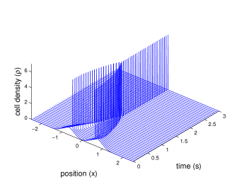
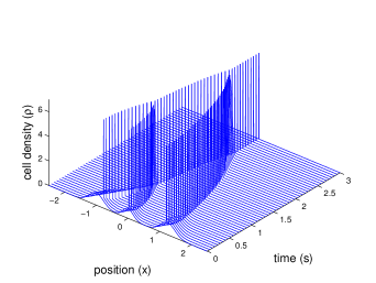
Figure 1: Dynamics of the density $\rho$ in the case $W=\frac{1}{2}(e^{-|x|}-1)$ and for a nonlinear function $a(x)=\frac{2}{\pi}\mbox{atan}(50x)$.

Example 2: In Figure 2 we display the time dynamics of the density $\rho$ for $W(x)=-\frac{|x|}{250}$ and $a(x)=\frac{2}{\pi}\mbox{atan}(50x)$. Contrary to the first example, we observe that the blow up occurs in the center and all bumps concentrate in this point to form a Dirac delta.

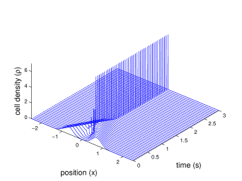
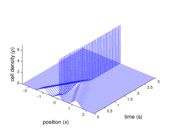
Figure 2: Dynamics of the density $\rho$ in the case $W=-\frac{|x|}{250}$ and for a nonlinear function $a(x)=\frac{2}{\pi}\mbox{atan}(50x)$.

Example 3: Finally, Figure 3 displays the time dynamics of the density $\rho$ when $W(x)=-\frac{|x|}{250}$ and in the linear case $a(x)=x$. In this last example, the bumps attract themselves and blow up in the same time. Then in Figure 3-left, with initial data (5.39), the blow up occurs when the two initial bumps are close to each other. In Figure 3-right, with initial data (5.40), the bump in the center blows up before the external ones.

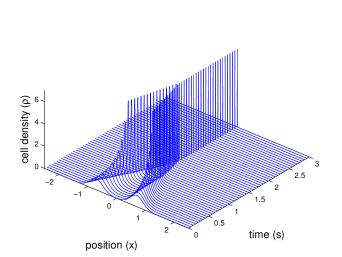
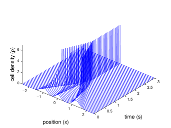
Figure 3: Dynamics of the density $\rho$ in the case $W=-\frac{|x|}{250}$ and when $a$ is linear.

References

• [1] L. Ambrosio, N. Gigli, and G. Savaré, Gradient Flows in Metric Space of Probability Measures, Lectures in Mathematics, Birkäuser, 2005
• [2] D. Benedetto, E. Caglioti, and M. Pulvirenti, A kinetic equation for granular media, RAIRO Model. Math. Anal. Numer., 31 (1997), 615-641.
• [3] A.L. Bertozzi, J.A. Carrillo, and T. Laurent, Blow-up in multidimensional aggregation equation with mildly singular interaction kernels, Nonlinearity 22 (2009), 683-710.
• [4] S. Bianchini, and M. Gloyer, An estimate on the flow generated by monotone operators, Comm. Partial Diff. Eq., 36 (2011), no 5, 777–796.
• [5] M. Bodnar, and J. J. L. Velázquez, An integro-differential equation arising as a limit of individual cell-based models, J. Differential Equations 222 (2006), no. 2, 341–380.
• [6] F. Bouchut, and F. James, One-dimensional transport equations with discontinuous coefficients, Nonlinear Analysis TMA, 32 (1998), no 7, 891–933.
• [7] F. Bouchut, and F. James, Duality solutions for pressureless gases, monotone scalar conservation laws, and uniqueness, Comm. Partial Differential Eq., 24 (1999), 2173–2189.
• [8] J. A. Carrillo, A. Chertock, and Y. Huang, A Finite-Volume Method for Nonlinear Nonlocal Equations with a Gradient Flow Structure, Comm. in Comp. Phys. 17 1 (2015), 233–258.
• [9] J. A. Carrillo, M. DiFrancesco, A. Figalli, T. Laurent, and D. Slepčev, Global-in-time weak measure solutions and finite-time aggregation for nonlocal interaction equations, Duke Math. J. 156 (2011), 229–271.
• [10] J. A. Carrillo, F. James, F. Lagoutière, and N. Vauchelet, The Filippov characteristic flow for the aggregation equation with mildly singular potentials, J. Differential Equations to appear
• [11] R.M. Colombo, M. Garavello, and M. Lécureux-Mercier, A class of nonlocal models for pedestrian traffic, Math. Models Methods Appl. Sci., (2012) 22(4):1150023, 34.
• [12] K. Craig, and A. L. Bertozzi, A blob method for the aggregation equation, Math. Comp. to appear.
• [13] Y. Dolak, and C. Schmeiser, Kinetic models for chemotaxis: Hydrodynamic limits and spatio-temporal mechanisms, J. Math. Biol., 51 (2005), 595–615.
• [14] F. Filbet, Ph. Laurençot, and B. Perthame, Derivation of hyperbolic models for chemosensitive movement, J. Math. Biol., 50 (2005), 189–207.
• [15] E. Godlewski, and P.-A. Raviart, Numerical approximation of hyperbolic systems of conservation laws, volume 118 of Applied Mathematical Sciences, Springer-Verlag, New York, 1996.
• [16] L. Gosse, and F. James, Numerical approximations of one-dimensional linear conservation equations with discontinuous coefficients, Math. Comput. 69 (2000) 987–1015.
• [17] A. Harten, On a class of high resolution total-variation-stable finite difference schemes SIAM Jour. of Numer. Anal. (1984), 21, 1–23.
• [18] F. James, and N. Vauchelet, A remark on duality solutions for some weakly nonlinear scalar conservation laws, C. R. Acad. Sci. Paris, Sér. I, 349 (2011), 657–661.
• [19] F. James, and N. Vauchelet, Chemotaxis: from kinetic equations to aggregation dynamics, Nonlinear Diff. Eq. and Appl. (NoDEA), 20 (2013), no 1, 101–127.
• [20] F. James, and N. Vauchelet, Equivalence between duality and gradient flow solutions for one-dimensional aggregation equations, Disc. Cont. Dyn. Syst., 36 no 3 (2016), 1355-1382.
• [21] F. James, and N. Vauchelet, Numerical method for one-dimensional aggregation equations, SIAM J. Numer. Anal., 53 no 2 (2015), 895–916.
• [22] R. Jordan, D. Kinderlehrer, and F. Otto, The variational formulation of the Fokker-Planck equation, SIAM J. Math. Anal., 29 (1998), 1–17.
• [23] A.-Y. Le Roux A numerical conception of entropy for quasi-linear equations Math. of Comp. 31, (1977) 848–872.
• [24] H. Li, and G. Toscani, Long time asymptotics of kinetic models of granular flows, Arch. Rat. Mech. Anal., 172 (2004), 407–428.
• [25] B. Maury, A. Roudneff-Chupin, and F. Santambrogio, A macroscopic Crowd Motion Model of the gradient-flow type, Math. Models and Methods in Applied Sci. Vol. 20, No. 10 (2010) 1787–1821.
• [26] J. Nieto, F. Poupaud, and J. Soler, High field limit for Vlasov-Poisson-Fokker-Planck equations, Arch. Rational Mech. Anal., 158 (2001), 29-59.
• [27] A. Okubo, and S. Levin, Diffusion and Ecological Problems: Modern Perspectives, Springer, Berlin, 2002.
• [28] F. Poupaud, Diagonal defect measures, adhesion dynamics and Euler equation, Methods Appl. Anal., 9 (2002), no 4, 533–561.
• [29] F. Poupaud, and M. Rascle, Measure solutions to the linear multidimensional transport equation with discontinuous coefficients, Comm. Partial Diff. Equ., 22 (1997), 337–358.
• [30] C. Villani, Topics in Optimal Transportation, Graduate Studies in Mathematics 58, Amer. Math. Soc, Providence, 2003.