A study of geodesic motion in a (2+1)–dimensional charged BTZ black hole

Abstract

This study is purposed to derive the equation of motion for geodesics in vicinity of spacetime of a $(2+1)$–dimensional charged BTZ black hole. In this paper, we solve geodesics for both massive and massless particles in terms of Weierstrass elliptic and Kleinian sigma hyper–elliptic functions. Then we determine different trajectories of motion for particles in terms of conserved energy and angular momentum and also using effective potential.

I INTRODUCTION

Black hole is one of the most interesting predictions of general theory of relativity which has been attractive for theoretical physicists for a long time, and it has still unknown parts to study.

Black hole is a region of spacetime with a strong gravitational field that even light can not escape from it. It has an event horizon which its total area never decreases in any physical process Singh:2014gva . In 1992 Banados, Teitelboim, and Zanelli (BTZ) demonstrated that there is a black hole solution to (2+1)–dimensional general relativity with a negative cosmological constant Banados:1992wn which it is proved that this type of black hole arises from collapsing matter Ross:1992ba . In their solution of gravitational field equation, it is required a constant curvature in local spacetime Horowitz:1993jc , which was a strange result as a solution of general relativity. In a certain subset of Anti–de Sitter (AdS) spacetime, they found a solution which contains all the properties of black hole, by making a special identification Horowitz:1993jc ,Banados:1992gq . Also, the charged BTZ black hole is the analogous solution of AdS–Maxwell gravity in (2+1)–dimension Martinez:1999qi ,Carlip:1995qv ,Clement:1995zt .

The BTZ black hole is interesting because of its connections with string theory Sfetsos:1997xs ,Hyun:1997jv and its role in microscopic entropy derivations Carlip:1994gy ,Carlip:1996yb . The BTZ black hole can also be used in some ways to study black holes in quantum scales Carlip:1995qv ,Strominger:1996sh . Against the Schwarzschild and Kerr black holes the BTZ black hole is asymptotically anti–de Sitter rather than flat which has not curvature singularity at the origin Carlip:1995qv .

Black holes have various aspects to study. One of them that we are more interested to investigate is the gravitational effects on test particles and light which reach to spacetime of a black hole. It is important because the motion of matter and light can be used to classify an arbitrary spacetime, in order to discover its structure. For this purpose, we need to solve geodesic equations that describe the motion of particles and light. The analytical solutions for many famous spacetimes (such as Schwarzschild Y.Hagihara:1931 , four-dimensional Schwarzschild-de-Sitter Hackmann:2008zz , higher–dimensional Schwarzschild, Schwarzschild–(anti)de Sitter, Reissner–Nordstrom and Reissner–Nordstrom–(anti)-de Sitter Hackmann:2008tu , Kerr Kerr:1963ud , Kerr–de Sitter Hackmann:2010zz , A black hole in f(R) gravity Soroushfar:2015wqa ) have been found previously. The solutions are given in terms of Weierstrass $\wp$-functions and derivatives of Kleinian sigma functions.

The interesting classical and quantum properties of the black hole, have made it appropriate to have existing a lower dimensional analogue that could represent the main features without unessential complications Banados:1992wn . Moreover, (2+1)-dimensional black holes are interesting as simplifed models for analyzing conceptual issues such as black hole thermodynamics Ashtekar:2002qc . In addition, the study of black holes in lower dimensions is useful to better understanding the physical features (like entropy, radiated flux) in a black hole geometry Sa:1995vs . Also, studying the gravitational field of (2+1)-dimensional black holes and motion around these black hole, can be useful.

The purpose in this paper is to determine types of particle’s motion around a (2+1)–dimensional charged BTZ black hole by studying its spacetime. The outline of our paper is as follows. In section II we introduce the metric and obtain geodesic equations. Section III includes analytical solutions for massless and massive particles and also the resulting orbits are classified in terms of the energy and the angular momentum of test particle, and we conclude in section IV.

II Metric and geodesic equations

The charged BTZ black hole is the solution of the (2+1)–dimensional Einstein-Maxwell gravity with a negative cosmological constant $\Lambda=-\frac{1}{l^{2}}$ Martinez:1999qi . In the case of a special matter source which is a nonlinear electrodynamic term in the form of $(F_{\mu\nu}~{}F^{\mu\nu})^{s}$, which is called Einstein-PMI gravity Hassaine:2008pw ; Maeda:2008ha ; Hendi:2009zzc , the form of the coupled (2+1)–dimensional action in presence of cosmological constant is written as follow Hendi:2010px

$$I(g_{\mu\nu},A_{\mu})=\frac{1}{16\pi}{\int}_{\partial M}d^{3}x\sqrt{-g}[R-2\Lambda+(kF)^{s}].$$ (1)

Here $R$ denotes the scalar curvature, $F$ is the Maxwell invariant which is equal to $F_{\mu\nu}F^{\mu\nu}$ ($F_{\mu\nu}=\partial_{\mu}A_{\nu}-\partial_{\nu}A_{\mu}$ is the electromagnetic tensor field and $A_{\mu}$ is the gauge potential), and $s$ is an arbitrary positive nonlinearity parameter ($s\neq\frac{1}{2}$). Varying the action (1) with respect to $g_{\mu\nu}$ (the metric tensor) and $A_{\mu}$ (the electromagnetic field), one can obtain the equations of gravitational and electromagnetic fields as

$$G_{\mu\nu}-\Lambda g_{\mu\nu}=T_{\mu\nu},$$ (2)

$$\partial_{\mu}(\sqrt{-g}F^{\mu\nu}(kF)^{s-1})=0,$$ (3)

and energy–momentum tensor is

$$T_{\mu\nu}=2[skF_{\mu\rho}F_{\nu}^{\rho}(kF)^{s-1}-\frac{1}{4}g_{\mu\nu}(kF)^{s}],$$ (4)

where $k$ is a constant. When $s$ and $k$ go to $-1$, Eqs.(1-4), reduce to the field equations of black hole in Einstein-Maxwell gravity. It is convenient to restrict the nonlinearity parameter to $s>\frac{1}{2}$ in order to have asymptotically well-defined electric field. The metric of non rotating charged BTZ black hole can be written as following Hendi:2014mba

$$ds^{2}=-g(r)dt^{2}+\frac{dr^{2}}{g(r)}+r^{2}d\phi^{2},$$ (5)

in which the metric function $g(r)$ using the components of Eq.(2) obtains as Hendi:2014mba

$$g(r)=\frac{r^{2}}{l^{2}}-m+\left\{\begin{array}[]{rl}{\ 2q^{2}ln(\frac{r}{l})}&s=1,\\ \\ \frac{(2s-1)^{2}(\frac{sq^{2}(s-1)^{2}}{(2s-1)^{2}})^{s}}{2(s-1)}r^{(\frac{2(s-1)}{2s-1})}&otherwise.\\ \end{array}\right.$$ (6)

This spacetime is characterized by $m$ (an integration constant related to the mass), $q$ (the electric charge of the black hole) and cosmological constant $\Lambda$. In the case of $s=\frac{3}{4}$, one can obtain a well-known metric which is called conformally invariant Maxwell solution Hendi:2014mba , such as

$$g(r)=\frac{r^{2}}{l^{2}}-m-\frac{(2q^{2})^{\frac{3}{4}}}{2r}.$$ (7)

Taking $(2q^{2})^{\frac{3}{4}}=K$ we have

$$ds^{2}=-(\frac{r^{2}}{l^{2}}-m-\frac{K}{2r})dt^{2}+\frac{dr^{2}}{\frac{r^{2}}{l^{2}}-m-\frac{K}{2r}}+r^{2}d\phi^{2}.$$ (8)

The metric (8) is stationay and axially symmetric. To describe geodesic motion in such a spacetime we need geodesic equation which is written as

$$\frac{d^{2}x^{\mu}}{d\lambda^{2}}+\Gamma_{\rho\sigma}^{\mu}\frac{dx^{\rho}}{d\lambda}\frac{dx^{\sigma}}{d\lambda}=0,$$ (9)

in which $d\lambda^{2}=g_{\mu\nu}dx^{\mu}dx^{\nu}$ is the proper time and $\Gamma_{\rho\sigma}^{\mu}$ denotes the Christoffel connections given by

$$\Gamma^{\mu}_{\rho\sigma}=\dfrac{1}{2}g^{\mu\nu}(\partial_{\rho}{g_{\sigma\nu}}+\partial_{\sigma}{g_{\rho\nu}}-\partial_{\nu}g_{\rho\sigma}).$$ (10)

We can obtain geodesic equations using Lagrangian equation

$$L=\frac{1}{2}\sum_{\mu,\nu=0}^{3}g_{\mu\nu}\frac{dx^{\mu}}{d\lambda}\frac{dx^{\nu}}{d\lambda}=\frac{1}{2}\epsilon=\frac{1}{2}[-(\frac{r^{2}}{l^{2}}-m-\frac{K}{2r})(\frac{dt}{d\lambda})^{2}+\frac{1}{(\frac{r^{2}}{l^{2}}-m-\frac{K}{2r})}(\frac{dr}{d\lambda})^{2}+r^{2}(\frac{d\phi}{d\lambda})^{2}],$$ (11)

where $\epsilon$ for massive and massless particles has the value of $1$ and $0$ respectively and $\lambda$ is an affine parameter.

Using Euler–Lagrange equation we can obtain constants of motion

$$P_{t}=\frac{\partial L}{\partial\dot{t}}=-(\frac{r^{2}}{l^{2}}-m-\frac{K}{2r})\dot{t}=-E\,\,\,,\,\,\,P_{\phi}=\frac{\partial L}{\partial\dot{\phi}}=r^{2}\dot{\phi}=\mathcal{L},$$ (12)

where $E$ is energy and $\mathcal{L}$ is angular momentum. Now, using Eq.(11) and Eq.(12), we can obtain geodesic equations as following

$$(\frac{dr}{d\lambda})^{2}=E^{2}+m\epsilon-\frac{\mathcal{L}^{2}}{l^{2}}-\frac{\epsilon r^{2}}{l^{2}}+\frac{K\epsilon}{2r}+\frac{m\mathcal{L}^{2}}{r^{2}}+\frac{K\mathcal{L}^{2}}{2r^{3}},$$ (13)

$$(\frac{dr}{d\phi})^{2}=(-\frac{\epsilon}{l^{2}\mathcal{L}^{2}})r^{6}+(\frac{E^{2}}{\mathcal{L}^{2}}+\frac{m\epsilon}{\mathcal{L}^{2}}-\frac{1}{l^{2}})r^{4}+(\frac{K\epsilon}{2\mathcal{L}^{2}})r^{3}+mr^{2}+\frac{Kr}{2}=R(r),$$ (14)

$$(\frac{dr}{dt})^{2}=(\frac{r^{2}}{l^{2}}-m-\frac{K}{2r})^{2}-\frac{\epsilon(\frac{r^{2}}{l^{2}}-m-\frac{K}{2r})^{3}}{E^{2}}-\frac{\mathcal{L}^{2}(\frac{r^{2}}{l^{2}}-m-\frac{K}{2r})^{3}}{E^{2}r^{2}}.$$ (15)

These equations give a complete description of dynamics. Using Eq.(13) we can find effective potential

$$V_{eff}=\frac{\epsilon r^{2}}{l^{2}}-\frac{K\epsilon}{2r}-\frac{m\mathcal{L}^{2}}{r^{2}}-\frac{K\mathcal{L}^{2}}{2r^{3}}-m\epsilon+\frac{\mathcal{L}^{2}}{l^{2}}.$$ (16)

Here for convenience we define a series of dimensionless parameters as

$$\tilde{r}=\frac{r}{m}\,\,,\,\,\tilde{l}=\frac{l}{m}\,\,,\,\,\tilde{K}=\frac{K}{m}\,\,,\,\,\tilde{\mathcal{L}}=\frac{m^{2}}{\mathcal{L}^{2}},$$ (17)

and then rewrite Eq.(14) as

$$(\frac{d\tilde{r}}{d\phi})^{2}={\tilde{r}}^{6}(\frac{-\epsilon\tilde{\mathcal{L}}}{\tilde{l}^{2}})+{\tilde{r}}^{4}(E^{2}\tilde{\mathcal{L}}+\epsilon\tilde{\mathcal{L}}m-\frac{1}{\tilde{l}^{2}})+\tilde{r}^{3}(\frac{\epsilon\tilde{\mathcal{L}}\tilde{K}}{2})+m\tilde{r}^{2}+\frac{\tilde{K}\tilde{r}}{2}=R(\tilde{r}).$$ (18)

Comparision to other cases of paremeter $s$

For $s=\frac{3}{2}$, the metric function is equal to $g(r)=\frac{r^{2}}{l^{2}}-m+Ar^{\frac{1}{2}}$, in which $A=4(\frac{3q^{2}}{32})^{\frac{3}{2}}$, so we have

$$(\frac{dr}{d\phi})^{2}=r^{6}(-\frac{\epsilon}{\mathcal{L}^{2}l^{2}})+r^{4}(\frac{E^{2}}{\mathcal{L}^{2}}+\frac{m\epsilon}{l^{2}\mathcal{L}^{2}}-\frac{1}{l^{2}})+r^{2}(-\frac{A\epsilon}{\mathcal{L}^{2}}+m)-Ar.$$ (19)

The solution of this equation is similar to Eq.(14) (i.e. for $s=\frac{3}{4}$, that, it is investigated completely in this paper).
In the case of $s=1$, the metric function $g(r)$ is

$$g(r)=\frac{r^{2}}{l^{2}}-m+2q^{2}\ln(\frac{r}{l}),$$ (20)

and so we have

$$(\frac{dr}{d\phi})^{2}=r^{6}(-\frac{\epsilon}{\mathcal{L}^{2}l^{2}})+r^{4}(\frac{E^{2}}{\mathcal{L}^{2}}+\frac{m\epsilon}{\mathcal{L}^{2}}-\frac{2\epsilon q^{2}}{\mathcal{L}^{2}}\ln(\frac{r}{l})-\frac{1}{l^{2}})+r^{2}(m-2q^{2}\ln(\frac{r}{l})),$$ (21)

and for $s=3$, the metric function is $g(r)=\frac{r^{2}}{l^{2}}-m+Qr^{\frac{4}{5}}$, where $Q=\frac{25(\frac{12q^{2}}{25})^{3}}{4}$, so we have

$$(\frac{dr}{d\phi})^{2}=r^{6}(-\frac{\epsilon}{\mathcal{L}^{2}l^{2}})+r^{4}(\frac{E^{2}}{\mathcal{L}^{2}}+\frac{m\epsilon}{\mathcal{L}^{2}}-\frac{1}{l^{2}})+mr^{2}-\frac{Q\epsilon}{\mathcal{L}^{2}}r^{\frac{24}{5}}-Qr^{\frac{14}{5}}.$$ (22)

Equation (21) includes some logarithmic terms, equation (22) and other equations related to other cases of $s$, have some terms with fractional powers of $r$, that, in our knowledge can not be solved analytically. However, they may be solved numerically similar to applied methods in Ref. Hartmann:2010rr . Therefore, in the following we consider the conformally invariant Maxwell solution ($s=\frac{3}{4}$).

Possible regions for Geodesic motion

Equation (18) implies that a necessary condition for the existence of a geodesic is $R(\tilde{r})\geq 0$, and therefore, the real positive zeros of $R(\tilde{r})$ are extremal values of the geodesic motion and determine the type of geodesic. Since $\tilde{r}=0$ is a zero of this polynomial for all values of the parameters, we can neglect it. So the Eq.(18) changes to a polynomial of degree $5$ as below

$$R^{*}(\tilde{r})={\tilde{r}}^{5}(\frac{-\epsilon\tilde{\mathcal{L}}}{\tilde{l}^{2}})+{\tilde{r}}^{3}(E^{2}\tilde{\mathcal{L}}+\epsilon\tilde{\mathcal{L}}m-\frac{1}{\tilde{l}^{2}})+\tilde{r}^{2}(\frac{\epsilon\tilde{\mathcal{L}}\tilde{K}}{2})+m\tilde{r}+\frac{\tilde{K}}{2}.$$ (23)

Using analytical solutions, one can analyze possible orbits which depend on the parameters of test particle or light ray $\epsilon$, $E^{2}$, $l$, $K$ and $\mathcal{L}$. In the next sections it will be shown exactly.

For a given set of parameters $\epsilon$, $l$, $E^{2}$, $K$ and $\mathcal{L}$ the polynomial $R^{*}(r)$ has a certain number of positive and real zeros. If $E^{2}$ and $\mathcal{L}$ are varied, the number of zeros can change only if two zeros of $R^{*}(r)$ merge to one. Solving $R^{*}(\tilde{r})=0$ and $\frac{dR^{*}(\tilde{r})}{d\tilde{r}}=0$ give us $E^{2}$ and $\mathcal{\tilde{L}}$. For massive particles $(\epsilon=1)$ we have

$$\tilde{\mathcal{L}}=-\frac{\tilde{l}^{2}(4m\tilde{r}+3\tilde{K})}{\tilde{r}^{2}(\tilde{K}\tilde{l}^{2}+4\tilde{r}^{3})}\,\,\,,\,\,\,E^{2}=-\frac{4\tilde{l}^{4}m^{2}\tilde{r}^{2}+4\tilde{K}\tilde{l}^{4}m\tilde{r}-8\tilde{l}^{2}m\tilde{r}^{4}+\tilde{K}^{2}\tilde{l}^{4}-4\tilde{K}\tilde{l}^{2}\tilde{r}^{3}+4\tilde{r}^{6}}{(4m\tilde{r}+3\tilde{K})\tilde{l}^{4}\tilde{r}},$$ (24)

and for massless particles $(\epsilon=0)$

$$\tilde{\mathcal{L}}=(-\frac{64m^{3}}{27\tilde{K}^{2}}+\frac{1}{\tilde{l}^{2}})\frac{1}{E^{2}}.$$ (25)

The results of this analysis are shown in Figs.(1), (2) in which regions of different types of geodesic motion are classified.

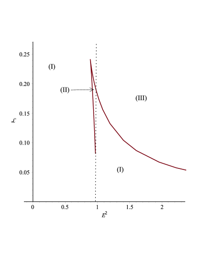
Figure 1: Region of different types of geodesic motion for test particles ($\epsilon=1$). The numbers of positive real zeros in these regions are: I=2, II=4, III=0.

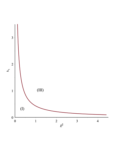
Figure 2: Region of different types of geodesic motion for light ($\epsilon=0$). The numbers of positive real zeros in these regions are: I=2, III=0.

The shape of an orbit is related to energy and angular momentum of test particle. Since $\tilde{r}$ must be real and positive, the acceptable physical regions can be found with the condition $E^{2}\geqslant V_{eff}$. So the number of positive and real zeros of $R(\tilde{r})$ will characterize the shape of different orbits. Here according to the obtained results in this section, we can identify three regions for geodesic motion of test particles:

1. In region I, $R^{*}(\tilde{r})$ has two real and positive zeros $(r_{1}<r_{2})$ which for $R^{*}(\tilde{r})\geq 0$ we have $0<\tilde{r}<r_{1}$ and $\tilde{r}\geq r_{2}$. There are two kinds of orbits, terminating bound orbit and flyby orbit (TBOs, FOs).

2. In region II, $R^{*}(\tilde{r})$ has four real positive zeros $(r_{i}<r_{i+1})$ that for $R^{*}(\tilde{r})\geq 0$ they are $0<\tilde{r}<r_{1}$, $r_{2}<\tilde{r}<r_{3}$ and $r_{4}\leq\tilde{r}$. Three possible orbits are terminating bound, bound and flyby orbits respectively (TBOs, BOs, FOs).

3. In region III, there is no real and positive zero for $R^{*}(\tilde{r})$ and $R^{*}(\tilde{r})\geq 0$ for positive $\tilde{r}$, therefore there is just terminating escape orbit (TEOs).

For timelike geodesics these three regions will appear but for null geodesics only regions I and III are exist. In Fig.3 different potentials for each of these regions are illustrated.

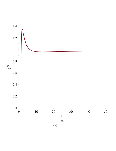
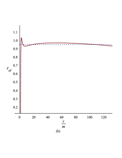
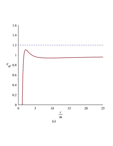
Figure 3: Effective potentials for different regions of geodesic motion for test particles (a: region I, b: region II, c: region III). The horizontal line denotes the squared energy parameter $E^{2}$.

III Analytical solution of geodesic equation

In this section we study analytical solutions of equations of motion. Using a new parameter $u=\frac{1}{\tilde{r}}$ we simplify Eq.(18) to

$$(\frac{du}{d\phi})^{2}=\frac{\tilde{K}u^{3}}{2}+mu^{2}+(\frac{\epsilon\tilde{\mathcal{L}}\tilde{K}}{2})u+(E^{2}\tilde{\mathcal{L}}+\epsilon\tilde{\mathcal{L}}m-\frac{1}{\tilde{l}^{2}})+(\frac{-\epsilon\tilde{\mathcal{L}}}{\tilde{l}^{2}})\frac{1}{u^{2}}.$$ (26)

We will consider it for both particle and light ray as following.

3.1) Null geodesics

For $\epsilon=0$ Eq.(26) changes to

$$(\frac{du}{d\phi})^{2}=\frac{\tilde{K}u^{3}}{2}+mu^{2}+(E^{2}\tilde{\mathcal{L}}-\frac{1}{\tilde{l}^{2}})=P_{3}(u)=\sum_{i=0}^{3}a_{i}u^{i},$$ (27)

which is of elliptic type. Another substitution $u=\frac{1}{a_{3}}(4y-\frac{a_{2}}{3})=\frac{2}{\tilde{K}}(4y-\frac{m}{3})$ transforms Eq.(27) into Weierstrass form as below

$$(\frac{dy}{d\phi})^{2}=4y^{3}-\alpha y-\gamma=P_{3}(y),$$ (28)

in which

$$\alpha=\frac{a_{2}^{2}}{12}-\frac{a_{1}a_{3}}{4}=\frac{m^{2}}{12}\,\,\,\,,\,\,\,\,\gamma=\frac{a_{1}a_{2}a_{3}}{48}-\frac{a_{0}a_{3}^{2}}{16}-\frac{a_{2}^{3}}{216}=-\frac{(E^{2}\tilde{\mathcal{L}}\tilde{l}^{2}-1)\tilde{K}^{2}}{64\tilde{l}^{2}}-\frac{m^{3}}{216},$$ (29)

are Weierstrass constants. The Eq.(28) is of elliptic type and is solved by the Weierstrass function Hackmann:2008zz , Soroushfar:2015wqa

$$y(\phi)=\wp(\phi-\phi_{in};\alpha,\gamma),$$ (30)

which here we have $\phi_{in}=\phi_{0}+\int_{y_{0}}^{\infty}\frac{dy}{\sqrt{4y^{3}-\alpha y-\gamma}}$ and $y_{0}=\frac{1}{4}(\frac{a_{3}}{\tilde{r}_{0}}+\frac{a_{2}}{3})=\frac{\tilde{K}}{8\tilde{r}_{0}}+\frac{m}{12}$ depends only on the initial values $\phi_{0}$ and $\tilde{r}_{0}$. As a result, the analytical solution of Eq.(18) is

$$\tilde{r}(\phi)=\frac{a_{3}}{4\wp(\phi-\phi_{in};\alpha;\gamma)-\frac{a_{2}}{3}}=\frac{\tilde{K}}{2[4\wp(\phi-\phi_{in};\alpha;\gamma)-\frac{m}{3}]}.$$ (31)

Using this solution we could create the examples of null geodesics for each region of different types of orbits which are plotted in Figs.4 and 5.

3.2) Timelike geodesics

For $\epsilon=1$ Eq.(26) changes to

$$(u\frac{du}{d\phi})^{2}=\frac{\tilde{K}u^{5}}{2}+mu^{4}+(\frac{\tilde{\mathcal{L}}\tilde{K}}{2})u^{3}+(E^{2}\tilde{\mathcal{L}}+\tilde{\mathcal{L}}m-\frac{1}{\tilde{l}^{2}})u^{2}-\frac{\tilde{\mathcal{L}}}{\tilde{l}^{2}}=P_{5}(u)=\sum_{i=1}^{5}a_{i}u^{i},$$ (32)

which is a polynomial of degree $5$ with an analytical solution as below Hackmann:2008zz ; Enolski:2010if ; Soroushfar:2015wqa

$$u(\phi)=-\frac{\sigma_{1}}{\sigma_{2}}(\phi_{\sigma}),$$ (33)

where $\sigma_{i}$ is the i-th derivative of the Kleinian sigma function in two variables

$$\sigma(z)=Ce^{-\frac{1}{2}z^{t}\eta\omega^{-1}z}\theta[g,h]((2\omega)^{-1}z;\tau).$$ (34)

We have some parameters here: the symmetric Riemann matrix $\tau=\omega^{-1}\acute{\omega}$, the Riemann theta-function $\theta[g,h]$, which is written as

$$\theta[g;h](z;\tau)=\sum_{m\in\mathbb{Z}^{g}}e^{i\pi(m+g)^{t}(\tau(m+g)+2z+2h)},$$ (35)

the period-matrix $(2\omega,2\acute{\omega})$, the period-matrix of the second type $(2\eta,2\acute{\eta})$, and $C$ is a constant that can be given explicitly. Note that $z$ is a zero of the Kleinian sigma function if and only if $(2\omega)^{-1}z$ is a zero of the theta-function $\theta[g,h]$.

With Eq.(33) the solution for $\tilde{r}$ is

$$\tilde{r}=-\frac{\sigma_{2}}{\sigma_{1}}(\phi_{\sigma}).$$ (36)

This solution of $\tilde{r}$ is the analytical solution of the equation of motion for massive particle. Different types of orbits for each region of this solution are illustrated in Figs.6–8.

III.1 Orbits

In region I, as we expressed before, there are two kinds of orbits ((TBO: $r$ starts in $(0,r_{a}]$ for $0<r_{a}<\infty$ and falls into the singulariry at $r=0$),(FO: $r$ starts from $\infty$, then approaches a periapsis $r=r_{p}$ and then goes back to $\infty$)) with $E^{2}=1.2$ and $\mathcal{L}=0.11$. In region II, we have three orbits ((TBO),(FO),(BO: $r$ oscillates between two boundary values $r_{p}\leq r\leq r_{a}$ with $0<r_{p}<r_{a}<\infty$)) with $E^{2}=0.95$ and $\mathcal{L}=0.17$. Region III has just one kind of orbit (TEO: $r$ comes from $\infty$ and falls into the singularity at $r=0$) with $E^{2}=1.2$ and $\mathcal{L}=0.15$. With the help of analytical solutions, parameter diagrams Figs. 1, 2 and effective potentials Fig. 3, various orbits for these three regions considering, $\Lambda=-\frac{1}{l^{2}}=\frac{1}{3}(10^{-5})$ and $q=1.25$, are presented in Figs. 4–8.

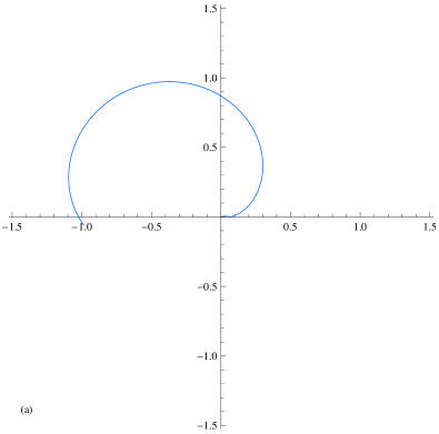
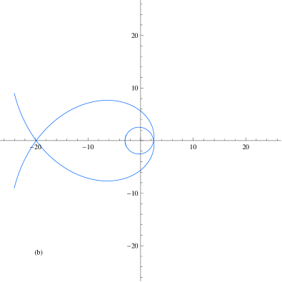
Figure 4: Null geodesic, Region I: (a) corresponding Terminating Bound Orbit with $E^{2}=0.3$, $\mathcal{L}=0.1$ , (b) corresponding Flyby Orbit with $E^{2}=0.9$, $\mathcal{L}=0.1$.

Figure 5: Null geodesic, Region III: corresponding Terminating Escape Orbit with $E^{2}=3$, $\mathcal{L}=0.3$.

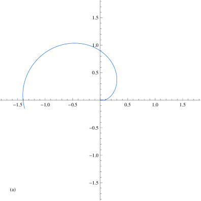
Figure 6: Timelike geodesic, Region I: (a) corresponding Terminating Bound Orbit with $E^{2}=1.2$, $\mathcal{L}=0.11$ , (b) corresponding Flyby Orbit with $E^{2}=1.6$, $\mathcal{L}=0.05$.

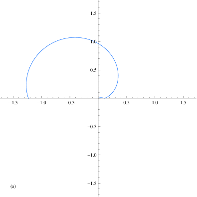
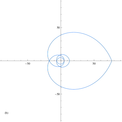
Figure 7: Timelike geodesic, Region II: (a) corresponding Terminating Bound Orbit with $E^{2}=0.965$, $\mathcal{L}=0.11$ , (b) corresponding Bound Orbit with $E^{2}=0.95$, $\mathcal{L}=0.17$, (c) corresponding Flyby Orbit with $E^{2}=0.95$, $\mathcal{L}=0.17$.

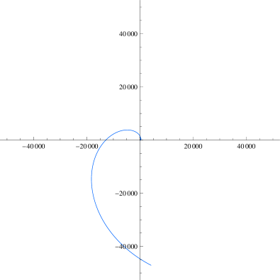
Figure 8: Timelike geodesic, Region III: Terminating Escape Orbit with $E^{2}=2.2$, $\mathcal{L}=0.15$.

IV Conclusion

In this paper, considering a three dimensional charged BTZ black hole, we studied the motion of particles (massive) and light rays (massless). For this purpose, at first we found equations of motion (geodesic equations), then using effective potential and solving geodesic equations in terms of Weierstrass elliptic function and Kleinian sigma hyper-elliptic function, we classified the complete set of orbit types. We also demonstrated that for both timelike and null geodesics there are different regions where test particles can move in. These regions and possible kinds of motion are illustrated in Figs. 1–8. For timelike geodesics TBO, BO, FO and TEO are possible and for null geodesics TBO, FO and TEO are possible.

These results and obtained figures can be used to have an intuition about the properties of the orbits such as light deflection, periastron shift and so on. The higher dimension and rotating version of this spacetime could be studied in future.

References

- (1) D. V. Singh and S. Siwach, J. Phys. Conf. Ser. 481, 012014 (2014).
- (2) M. Banados, C. Teitelboim and J. Zanelli, Phys. Rev. Lett. 69, 1849 (1992) [hep-th/9204099].
- (3) S. F. Ross and R. B. Mann, Phys. Rev. D 47, 3319 (1993) [hep-th/9208036].
- (4) G. T. Horowitz and D. L. Welch, Phys. Rev. Lett. 71, 328 (1993) [hep-th/9302126].
- (5) M. Banados, M. Henneaux, C. Teitelboim and J. Zanelli, Phys. Rev. D 48, 1506 (1993) [Phys. Rev. D 88, no. 6, 069902 (2013)] [gr-qc/9302012].
- (6) C. Martinez, C. Teitelboim and J. Zanelli, Phys. Rev. D 61, 104013 (2000) [hep-th/9912259].
- (7) S. Carlip, Class. Quant. Grav. 12, 2853 (1995) [gr-qc/9506079].
- (8) G. Clement, Phys. Lett. B 367, 70 (1996) [gr-qc/9510025].
- (9) K. Sfetsos and K. Skenderis, Nucl. Phys. B 517, 179 (1998) [hep-th/9711138].
- (10) S. Hyun, J. Korean Phys. Soc. 33, S532 (1998) [hep-th/9704005].
- (11) S. Carlip, Phys. Rev. D 51, 632 (1995) [gr-qc/9409052].
- (12) S. Carlip, Phys. Rev. D 55, 878 (1997) [gr-qc/9606043].
- (13) A. Strominger and C. Vafa, Phys. Lett. B 379, 99 (1996) [hep-th/9601029].
- (14) Y.Hagihara. Theory of relativistic trajectories in a gravitational field of Schwarzschild .( Japan. J. Astron.Geophys., 8:67, 1931).
- (15) E. Hackmann and C. Lammerzahl, Phys. Rev. D 78, 024035 (2008) [arXiv:1505.07973 [gr-qc]].
- (16) E. Hackmann, V. Kagramanova, J. Kunz and C. Lammerzahl, Phys. Rev. D 78, 124018 (2008); Phys. Rev. D 79, 029901 (E) (2009) [arXiv:0812.2428 [gr-qc]].
- (17) R. P. Kerr, Phys. Rev. Lett. 11, 237 (1963).
- (18) E. Hackmann, C. Lammerzahl, V. Kagramanova and J. Kunz, Phys. Rev. D 81, 044020 (2010) [arXiv:1009.6117 [gr-qc]].
- (19) S. Soroushfar, R. Saffari, J. Kunz and C. Lämmerzahl, Phys. Rev. D 92, 044010 (2015) [arXiv:1504.07854 [gr-qc]].
- (20) A. Ashtekar, J. Wisniewski and O. Dreyer, Adv. Theor. Math. Phys. 6, 507 (2003) [gr-qc/0206024].
- (21) P. M. Sa, A. Kleber and J. P. S. Lemos, Class. Quant. Grav. 13, 125 (1996) [hep-th/9503089].
- (22) M. Hassaine and C. Martinez, Class. Quant. Grav. 25, 195023 (2008) [arXiv:0803.2946 [hep-th]].
- (23) H. Maeda, M. Hassaine and C. Martinez, Phys. Rev. D 79, 044012 (2009) [arXiv:0812.2038 [gr-qc]].
- (24) S. H. Hendi, Phys. Lett. B 678, 438 (2009) [arXiv:1007.2476 [hep-th]].
- (25) S. H. Hendi, Eur. Phys. J. C 71, 1551 (2011) [arXiv:1007.2704 [gr-qc]].
- (26) S. H. Hendi, B. Eslam Panah and R. Saffari, Int. J. Mod. Phys. D 23, 1450088 (2014) [arXiv:1408.5570 [hep-th]].
- (27) B. Hartmann and P. Sirimachan, JHEP 1008, 110 (2010) doi:10.1007/JHEP08(2010)110 [arXiv:1007.0863 [gr-qc]].
- (28) V. Z. Enolski, E. Hackmann, V. Kagramanova, J. Kunz and C. Lammerzahl, J. Geom. Phys. 61, 899 (2011) [arXiv:1011.6459 [gr-qc]].