Preweighting method in Monte-Carlo sampling with complex action
— Strong-Coupling Lattice QCD with $1/g^{2}$ corrections, as an example —

Abstract:

We investigate the QCD phase diagram in the strong-coupling lattice QCD with fluctuation and $1/g^{2}$ effects by using the auxiliary field Monte-Carlo simulations. The complex phase of the Fermion determinant at finite chemical potential is found to be suppressed by introducing a complex shift of integral path for one of the auxiliary fields, which corresponds to introducing a repulsive vector mean field for quarks. The obtained phase diagram in the chiral limit shows suppressed $T_{c}$ in the second order phase transition region compared with the strong-coupling limit results. We also argue that we can approximately guess the statistical weight cancellation from the complex phase in advance in the case where the complex phase distribution is Gaussian. We demonstrate that correct expectation values are obtained by using this guess in the importance sampling (preweighting).

1 Introduction

QCD phase diagram is closely related to compact star phenomena and can be accessed using heavy-ion collisions. It is desirable to understand the QCD phase diagram in non-perturbative first-principles theory, i.e. lattice QCD Monte-Carlo (LQCD-MC) simulations, but LQCD-MC suffers from the sign problem at finite chemical potential ($\mu$). There are many methods proposed so far to circumvent the sign problem, but it is still difficult to attack low temperature ($T$) QCD matter.

The strong coupling lattice QCD (SC-LQCD) is one of the methods, with which the phase boundary has been drawn using QCD [1, 2, 3, 4, 5, 6]. In SC-LQCD, (spatial) link variables are integrated out first, and we obtain the effective action consisting of color singlet composites to a given order of $1/g^{2}$. Then fluctuations of the complex phase from the link fluctuations could be suppressed, namely the sign problem becomes milder. For example, there is no sign problem in the mean field treatment [1, 2], and the phase diagram has been obtained in the strong coupling limit ($\mathcal{O}(1/g^{0})$) [1] as well as with finite coupling effects [2]. The sign problem appears when we include fluctuation effects, but it is not severe in the strong coupling limit. The phase boundary in the strong coupling limit with fluctuation effects has been obtained in two independent method, the Monomer-Dimer-Polymer (MDP) simulations [3] and the Auxiliary Field Monte-Carlo (AFMC) method [4], and obtained phase boundaries agree with each other. Towards the actual QCD phase diagram, we need to take account of both finite coupling and fluctuation effects. Recently, the plaquette effects on the phase boundary were evaluated using the linear and exponential extrapolation in the MDP simulation [5]. In AFMC, an effective action including $1/g^{2}$ contributions was considered, but the sign problem was found to be severe [7]. Thus the direct sampling method including the finite coupling corrections should be further developed.

Another interesting technique to avoid the sign problem has been developed in the density of states method [8, 9, 10]. If the complex phase $\theta$ follows a Gaussian distribution, as examined in the heavy quark mass region [9], we can integrate out $\theta$ and obtain the partition function without the sign problem. It is desirable to examine the $\theta$ distribution at small quark masses. Furthermore, it is preferable to judge the statistical weight in advance in order to enhance numerical efficiency.

In this proceedings, we discuss the QCD phase transition in SC-LQCD with fluctuation and $1/g^{2}$ effects by using the AFMC method. We introduce two ideas to suppress the complex phase spread; the complex shift of auxiliary field integration path and the preweighting.

2 Auxiliary Field Monte-Carlo method in SC-LQCD with $1/g^{2}$ corrections

We here consider the lattice QCD with one species of unrooted staggered fermion in the anisotropic Euclidean spacetime. Throughout this paper, we work in the lattice unit $a=1$, where $a$ is the spatial lattice spacing, and the case of color $\mathrm{SU}(N_{c}=3)$ in 3+1 dimension $(d=3)$ spacetime. Temporal and spatial lattice sizes are denoted as $N_{\tau}$ and $L$, respectively.

Starting from the lattice QCD partition function, we obtain the effective action including the leading order (strong coupling limit (SCL), $\mathcal{O}(1/g^{0})$) terms and next-to-leading order (NLO, $1/g^{2}$) corrections by integrating out spatial link variables [1, 2, 4, 11, 12, 13],

$$S_{\mathrm{eff}}= \frac{1}{2}\sum_{x}\left[V^{+}_{x}(\mu)-V^{-}_{x}(\mu)\right]-\frac{1}{4N_{c}\gamma^{2}}\sum_{x,j}M_{x}M_{x+\hat{j}}+\frac{m_{0}}{\gamma}\sum_{x}M_{x}\ ,$$

$$+ \frac{\beta_{\tau}}{2}\sum_{x,j}\left[V_{x}^{+}(\mu)\,V^{-}_{x+\hat{j}}(\mu)+V_{x+\hat{j}}^{+}(\mu)\,V^{-}_{x}(\mu)\right]-\frac{\beta_{s}}{\gamma^{4}}\sum_{x,k,j,k\not=j}Q^{(j)}_{x}Q^{(j)}_{x+\hat{k}}\ ,$$ (1)

$$V^{+}_{x}(\mu)= \bar{\chi}_{x}e^{\mu/\gamma^{2}}U_{0,x}\chi_{x+\hat{0}}\ ,\ V^{-}_{x}(\mu)=\bar{\chi}_{x+\hat{0}}e^{-\mu/\gamma^{2}}U^{\dagger}_{0,x}\chi_{x}\ ,\ M_{x}=\bar{\chi}_{x}\chi_{x}\ ,\ Q^{(j)}_{x}=M_{x}M_{x+\hat{j}}\ ,$$ (2)

where $\chi_{x}$ and $U_{0,x}$ represent the quark field and the temporal link variable, respectively, $V^{\pm}_{x}$, $M_{x}$ and $Q^{(j)}_{x}$ are mesonic composites, $\beta_{\tau}=\beta_{g}/4N_{c}^{3}\gamma$, and $\beta_{s}=\beta_{g}/32N_{c}^{5}\gamma$, where $\beta_{g}=2N_{c}/g^{2}$. We assume that the physical lattice spacing ratio is given as a function of the lattice anisotropy parameter $\gamma$ as $f(\gamma)=a_{\mathrm{s}}^{\mathrm{phys}}/a_{\tau}^{\mathrm{phys}}=\gamma^{2}$, then the temperature is given as $T=\gamma^{2}/N_{\tau}$ [1].

We obtain the effective action of quarks, temporal link variables, and auxiliary fields in the bilinear form of quarks, by applying the extended Hubbard-Stratonovich (EHS) transformation $\exp(\alpha AB)=\int d\phi d\phi^{*}\exp[-\alpha(\phi^{*}\phi+\phi^{*}A+\phi B)]$ several times,

$$S_{\mathrm{EHS}}= \frac{1}{2}\sum_{x}\left(Z^{-}_{x}V_{x}^{+}-Z^{+}_{x}V_{x}^{-}\right)+\frac{1}{\gamma}\sum_{x}m_{x}M_{x}+S_{\mathrm{AF}}\ ,$$ (3)

$$m_{x}= m_{0}+\frac{1}{4N_{c}}\sum_{j}(\sigma+i\varepsilon\pi)_{x\pm\hat{j}}+\beta_{s}\sum_{j}\left\{\varphi^{(j)*}_{x}(\Theta_{x}^{(j)})^{1/2}+\varphi^{(j)*}_{x-\hat{j}}(\Theta_{x-\hat{j}}^{(j)})^{1/2}\right\}\ ,$$

$$Z^{-}_{x}= 1+\beta_{\tau}\sum_{j}(\omega-\varepsilon\Omega)_{x\pm\hat{j}}^{*}\ ,\quad Z^{+}_{x}=1+\beta_{\tau}\sum_{j}(\omega+\varepsilon\Omega)_{x\pm\hat{j}}\ ,\quad\Theta^{(j)}_{x}=\sum_{k,k\not=j}(\sigma^{(j)}+i\varepsilon\pi^{(j)})_{x\pm\hat{k}}\ ,$$

$$S_{\mathrm{AF}}= \frac{L^{3}}{4N_{c}}\sum_{\mathbb{k},\tau,f(\mathbb{k})>0}f(\mathbb{k})\left[\sigma^{*}_{\mathbb{k},\tau}\sigma_{\mathbb{k},\tau}+\pi^{*}_{\mathbb{k},\tau}\pi_{\mathbb{k},\tau}\right]+\beta_{\tau}L^{3}\sum_{\mathbb{k},\tau,f(\mathbb{k})>0}f(\mathbb{k})\left[\Omega_{\mathbb{k},\tau}^{*}\Omega_{\mathbb{k},\tau}+\omega_{\mathbb{k},\tau}^{*}\omega_{\mathbb{k},\tau}\right]$$

$$+\beta_{s}L^{3}\sum_{\mathbb{k},\tau,f^{(j)}(\mathbb{k})>0}f^{(j)}(\mathbb{k})\left[\sigma^{(j)*}_{\mathbb{k},\tau}\sigma^{(j)}_{\mathbb{k},\tau}+\pi^{(j)*}_{\mathbb{k},\tau}\pi^{(j)}_{\mathbb{k},\tau}\right]+\beta_{s}\sum_{x,j}\varphi^{(j)*}_{x}\varphi^{(j)}_{x}\ ,$$

where $f(\mathbb{k})=\sum_{j}\cos k_{j}$ and $f^{(j)}(\mathbb{k})=\sum_{k,k\not=j}\cos k_{k}$. SCL fields $(\sigma,\pi)$, spatial $(\sigma^{(j)},\pi^{(j)})$ and temporal $(\Omega,\omega)$ NLO fields are introduced to bosonize interaction terms, $M_{x}M_{x+\hat{j}}$, $Q^{(j)}_{x}Q^{(j)}_{x+\hat{k}}$, and $V^{+}_{x}V^{-}_{x+\hat{j}}+V^{+}_{x+\hat{j}}V^{-}_{x}$ terms in Eq. (1), respectively. The other spatial NLO field $\varphi^{(j)}$ is introduced in the second step bosonization of the eight-Fermi term, $Q^{(j)}_{x}Q^{(j)}_{x+\hat{k}}$. It should be noted that $\sigma$, $\pi$, $\sigma^{(j)}$ and $\pi^{(j)}$ fields are real in the coordinate representation.

We can integrate out quarks and temporal links analytically, and the partition function and the effective action in AFMC are found to be,

$$\mathcal{Z}_{\mathrm{AFMC}}= \int\mathcal{D}\Phi\exp\left(-S_{\mathrm{AFMC}}[\Phi]\right)\quad(\Phi=\left\{\sigma,\pi,\sigma^{(j)},\pi^{(j)},\varphi,\varphi^{*},\Omega,\Omega^{*},\omega,\omega^{*}\right\})\ ,$$ (4)

$$S_{\mathrm{AFMC}}= S_{\mathrm{AF}}-\sum_{\mathbb{x}}\log\left[R(\mathbb{x})\right]\ ,\quad R(\mathbb{x})=Z^{3}\left[(X_{N_{\tau}}/Z)^{3}-2(X_{N_{\tau}}/Z)+2\cosh(N_{c}\widetilde{\mu}/T)\right]\ ,$$ (5)

where $Z=[\prod_{\tau}Z_{\mathbb{x},\tau}^{-}Z_{\mathbb{x},\tau}^{+}]^{1/2}$ and $\widetilde{\mu}/T=\mu/T+\frac{1}{2}\sum_{\tau}\log\left(Z_{\mathbb{x},\tau}^{-}/Z_{\mathbb{x},\tau}^{+}\right)$. $X_{N_{\tau}}$ is obtained by using the recursion formula, $X_{N}(1;N)=B_{N}(1;N)+\gamma_{N}B_{N-2}(2;N-1)$, $B_{N}(1;N)=I_{N}B_{N-1}(1;N-1)+\gamma_{N-1}B_{N-2}(1;N-2)\ (N>3)$, $B_{1}(1;1)=I_{1}$, and $B_{2}(1;2)=I_{1}I_{2}+\gamma_{1}$, where $I_{\tau}=2m_{\mathbb{x},\tau}/\gamma$ and $\gamma_{\tau}=Z^{-}_{\mathbb{x},\tau}Z^{+}_{\mathbb{x},\tau}$ [12].

We now perform Monte-Carlo calculation using the auxiliary field effective action Eq. (5). We have made calculations at $\beta_{g}=0,1,2,3$ on $4^{3}\times 4$ and $6^{3}\times 4$ lattices in the chiral limit ($m_{0}=0$). In the left panel of Fig. 1, we show the chiral condensate at $\mu=0$ as a function of $T$ on a $4^{3}\times 4$ lattice at $\beta_{g}=0,1,2,3$ in comparison with the mean field results on anisotropic lattice with $N_{\tau}=4$. We define the chiral circle radius $\phi=\sqrt{\sigma^{2}_{k=0}+\pi^{2}_{k=0}}$ as the chiral condensate, since we work in the chiral limit. The chiral condensate is suppressed from the mean field results, and it roughly corresponds to the mean field result at $T_{\mathrm{MF}}=T/0.93$. In the right panel of Fig. 1, we show the critical temperature $T_{c}$ as a function of $\beta_{g}$. We have made a function fit to the chiral condensate in AFMC, and the critical temperature is defined as the maximum of $-d\phi/dT$ of the fitted function. The behavior of $T_{c}$ is again consistent with the scaled mean field results on an anisotropic lattice, $T_{c}(\mathrm{AFMC})\simeq 0.89T_{c}(\mathrm{MF,aniso.},N_{\tau}=4)$.

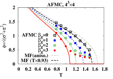
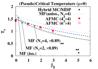
Figure 1: Chiral condensate (left) and critical temperature (right) at $\mu=0$.

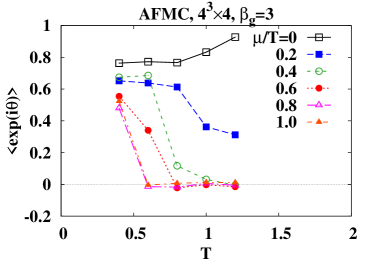
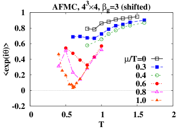
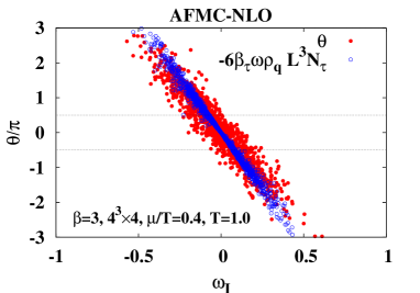
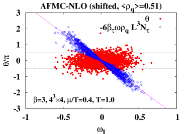
Figure 2: Average phase factor (upper panels) and correlation between $\omega_{I}$ and the complex phase (lower panels) in the original (left) and subtracted (right) action.

We have a sign problem in AFMC coming from the bosonization; decomposing the product of different composites requires introducing complex fields, as seen in the position dependent mass $m_{x}$ in Eq. (3), then the fermion determinant becomes a complex number. As shown in the upper left panel of Fig. 2, the average phase factor at $\mu/T=0$ is large enough, $\langle\exp(i\theta)\rangle>0.7$. At $\mu/T>0.4$, however, it suddenly collapses at around $T\sim 0.7$. This collapse comes from finite density. Let us examine this point. We focus our attention to those terms involving the imaginary part of $\omega$ at zero momentum in the EHS action Eq. (3),

$$S_{\omega_{I}}=\frac{1}{2}C\omega_{I}^{2}+iC\omega_{I}\rho_{q}\ \quad(C=6\beta_{\tau}L^{3}N_{\tau})\ ,$$ (6)

where $\omega_{I}=\sum_{\tau}\mathrm{Im}\omega_{\mathbb{k}=0,\tau}/N_{\tau}$, and $\rho_{q}$ is the quark number density. When $\rho_{q}$ is finite, the above term gives rise to a complex phase of $\theta=-C\omega\rho_{q}$. As shown in the lower left panel of Fig. 2, the above term dominates the complex phase. Fortunately, this sign problem is a kind of textbook example; By shifting the integral path to the imaginary direction $\omega_{I}\to\omega_{I}-i\rho_{q}$, we can remove the imaginary part $S_{\omega_{I}}\to C\omega_{I}^{2}/2+C\rho_{q}^{2}/2$. We tune the shift constant $\langle\rho_{q}\rangle$ for each $(T,\mu)$ carefully, then $\theta$ is suppressed and $\langle\exp(i\theta)\rangle$ becomes larger as shown in the right panels of Fig. 2.

We show the phase boundary at $\beta_{g}=3$ in the left panel of Fig. 3, in comparison with the phase boundary in SCL. The phase boundary at small $\mu/T$ seems to be flatter compared with the SCL boundary. This is consistent with the previous results [5, 7]. At $\mu/T>1$ where the first order phase transition would appear, a constant shift is not enough. When the high-density Wigner phase and the low-density Nambu-Goldstone phase coexist, we need to introduce configuration dependent shifts. Work in this direction is in progress.

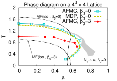
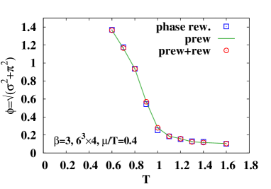
Figure 3: Phase diagram in SC-LQCD with $1/g^{2}$ correction at $\beta_{g}=3$ (left) and the chiral condensate in preweighting and reweighting (right).

3 Preweighting

For a calculation on larger lattices, complex shift of the integration path of one auxiliary field is not enough. One of the ideas to circumvent the sign problem is to apply the density of states approach [8, 9, 10], where we obtain the density of states for a given variable $x$, and evaluate the average phase factor in each bin of $x$. Leading order truncation of the cumulant expansion in $\theta$ corresponds to assuming that the complex phase distribution is Gaussian [9]. If this is the case, we can analytically integrate out $\theta$ and avoid the sign problem. Let us assume that the effective action is quadratic in $\theta$, $S[\Phi,\theta]=S_{\Phi}+\theta^{2}/2\Delta^{2}_{\Phi}-i\theta$, then the partition function is calculated as

$$\mathcal{Z}= \int\mathcal{D}\Phi d\theta\,e^{-S[\Phi,\theta]}=\int\mathcal{D}\Phi\,\sqrt{2\pi}\Delta_{\Phi}\,e^{-S_{\Phi}-\Delta^{2}_{\Phi}/2}\ ,$$ (7)

where $\Phi$ shows variables other than $\theta$, and $\Delta^{2}_{\Phi}$ is a variance of $\theta$ depending on $\Phi$. In the heavy-quark mass case, the complex phase $\theta$ was evaluated by using the Taylor expansion, and the reweighted $\theta$ distribution was examined to be well approximated by a Gaussian [9]. In order to generate MC samples at finite $\mu$ directly, we have an overlap problem and a problem of numerical cost. In standard phase quenched lattice QCD simulations, ignoring the complex phase leads to misidentification of $U$ and $U^{\dagger}$ and of pions and diquarks. The misidentification gives rise to the overlap problem; the appearance of pion condensed phase and superposed Lorentzian distribution of $\theta$ [14] at $\mu>m_{\pi}/2$ at low temperature, instead of baryonic matter. In SC-LQCD, we integrate out link variables analytically, and the pion condensed phase does not appear. By comparison, the cost problem remains. Configurations of $\Phi$ with large $\Delta^{2}_{\Phi}$ are suppressed by the factor $\exp(-\Delta^{2}_{\Phi}/2)$, but we do not know $\Delta^{2}_{\Phi}$ in advance.

Let us now introduce a preweighting factor, which suppresses configurations with large $\theta$,

$$\mathcal{Z}_{\mathrm{prew}}\equiv \int\mathcal{D}\Phi\,d\theta\,e^{-S_{\Phi}-\theta^{2}/2\Delta^{2}_{\Phi}}e^{-f(\theta)}=\int\mathcal{D}\Phi\,e^{-S_{\Phi}}F(\Delta_{\Phi})\ ,$$ (8)

where $F(\Delta)=\int d\theta\,e^{-\theta^{2}/2\Delta^{2}-f(\theta)}$. If we find a function $f(\theta)$ which satisfies $F(\Delta)/\sqrt{2\pi}\Delta=\exp(-\Delta^{2}/2)$, we can obtain a correct partition function. For small values of $\Delta$, the preweighting function $f(\theta)=\theta^{2}/2+\theta^{4}/12+\theta^{6}/45+17\theta^{8}/1260+\mathcal{O}(\theta^{10})$, is found to give a good approximation, $F(\Delta)/\sqrt{2\pi}\Delta=\exp(-\Delta^{2})+\mathcal{O}(\Delta^{10})$. Since $F(\Delta)$ becomes a constant at large $\Delta$, $F(\Delta)\to\int d\theta e^{-f}\ (\Delta\to\infty)$, and the preweighting partition function deviates from the correct one, we need to perform reweighting afterwards. We first obtain configurations in phase-quenched importance sampling with the preweighting factor, and calculate observables $\langle\hat{\phi}\rangle$ with the reweighting method, $\langle\hat{\phi}\rangle=\sum_{n}\phi_{n}R(\Delta_{n})/\sum_{n}R(\Delta_{n})$ with $R(\Delta)=\sqrt{2\pi}\Delta\,e^{-\Delta^{2}}/F(\Delta)$, where $n$ denotes one configuration and the variance $\Delta_{n}^{2}$ is obtained in a bin of $\phi$ to which $\phi_{n}$ belongs.

We have applied the preweighting + reweighting to SC-LQCD with $1/g^{2}$ corrections. We have confirmed that the complex phase distribution is approximated by Gaussian. In the right panel of Fig. 3 we show calculated results of chiral condensate $\phi$. Since the complex shifted path is applied and the complex phase variance is small in this case, the results of the phase reweighting, preweighting, and preweighting+reweighting agree with each other. Comparison under more severe condition would be necessary to verify the usefulness of the preweighting method.

4 Summary

In this proceedings, we have investigated the QCD phase diagram by using the auxiliary field Monte-Carlo simulations of the strong-coupling lattice QCD with $1/g^{2}$ corrections. We have found that a complex shift of integral path for one of the auxiliary fields ($\omega_{I}$) suppresses the complex phase of the Fermion determinant at finite $\mu$, which corresponds to introducing a repulsive vector mean field for quarks. The obtained phase diagram in the chiral limit shows suppressed $T_{c}$ in the second order phase transition region compared with the strong-coupling limit results. as suggested in previous works using the mean field approximation [2] and the reweighting method in the monomer-dimer-polymer simulations [5]. We have also proposed a preweighting method. When the distribution of the complex phase $\theta$ is Gaussian and the variance of $\theta$ is small, we can obtain a correct expectation value of an observable from the phase quenched configurations obtained by introducing the preweighting factor in the sampling process. We need to combine preweighting and reweighting in the large variance cases. We have demonstrated that the preweighting+reweighting works well.

This work is supported in part by JSPS/MEXT Grant Numbers 24540271, 15H03663, 15K05079, 24105001, and 24105008. TI is supported by the Grants-in-Aid for JSPS Fellows (No.25-2059).

References

- [1] E. M. Ilgenfritz, J. Kripfganz, Z. Phys. C29 (1985), 79; N. Bilic, F. Karsch, and K. Redlich, Phys. Rev. D 45 (1992), 3228; K. Fukushima, Prog. Theor. Phys. Suppl. 153 (2004), 204; Y. Nishida, Phys. Rev. D 69 (2004), 094501; N. Kawamoto, K. Miura, A. Ohnishi and T. Ohnuma, Phys. Rev. D 75 (2007) 014502.
- [2] K. Miura, T. Z. Nakano and A. Ohnishi, Prog. Theor. Phys. 122 (2009), 1045; K. Miura, T. Z. Nakano, A. Ohnishi and N. Kawamoto, Phys. Rev. D 80 (2009), 074034; T. Z. Nakano, K. Miura and A. Ohnishi, Prog. Theor. Phys. 123 (2010), 825; Phys. Rev. D 83, 016014 (2011).
- [3] F. Karsch and K. H. Mutter, Nucl. Phys. B 313 (1989), 541. P. de Forcrand and M. Fromm, Phys. Rev. Lett. 104 (2010), 112005; W. Unger and P. de Forcrand, J. Phys. G 38 (2011), 124190.
- [4] T. Ichihara, A. Ohnishi and T. Z. Nakano, PTEP 2014 (2014), 123D02;
- [5] P. de Forcrand, J. Langelage, O. Philipsen and W. Unger, Phys. Rev. Lett. 113 (2014), 152002.
- [6] C. S. Fischer and J. Luecker, Phys. Lett. B 718 (2013), 1036.
- [7] T. Ichihara, A. Ohnishi, PoS LATTICE2014 (2014), 188.
- [8] A. Gocksch, Phys. Rev. Lett. 61 (1988), 2054; K. N. Anagnostopoulos and J. Nishimura, Phys. Rev. D 66 (2002), 106008; Z. Fodor, S. D. Katz and C. Schmidt, JHEP 0703 (2007), 121.
- [9] S. Ejiri, Phys. Rev. D 77 (2008), 014508; Phys. Rev. D 78 (2008), 074507; S. Ejiri et al. [WHOT-QCD Collaboration], Phys. Rev. D 82 (2010) 014508.
- [10] J. Greensite, J. C. Myers and K. Splittorff, PoS LATTICE 2013 (2014), 023.
- [11] H. Kluberg-Stern, A. Morel, O. Napoly and B. Petersson, Nucl. Phys. B 190 (1981), 504; N. Kawamoto, Nucl. Phys. B 190 (1981), 617; H. Kluberg-Stern, A. Morel, B. Petersson, Nucl. Phys. B 215 [FS7] (1983), 527; N. Kawamoto and J. Smit, Nucl. Phys. B192 (1981), 100; P. H. Damgaard, N. Kawamoto and K. Shigemoto, Phys. Rev. Lett. 53 (1984), 2211.
- [12] G. Faldt and B. Petersson, Nucl. Phys. B 265 (1986), 197.
- [13] T. Jolicoeur, H. Kluberg-Stern, M. Lev, A. Morel, and B. Petersson, Nucl. Phys. B 235 (1984), 455.
- [14] M. P. Lombardo, K. Splittorff and J. J. M. Verbaarschot, Phys. Rev. D 80 (2009), 054509.