Polysymplectic Integrator
for the Short Pulse Equation

Abstract

The polysymplectic analysis of the Short Pulse Equation known in nonlinear optics is used in order to construct a geometric polysymplectic integrator for it. The proposed scheme turn out to be much more effective than other standard integration schemes for nonlinear PDEs, such as the pseudo-spectral integrator. In our numerical experiments the polysymplectic integrator appears to be an order of magnitude more precise and approximately 2.5 times faster at long propagation times than the pseudo-spectral method.

1 Introduction

The multisymplectic Hamiltonian formalism has emerged from geometric theories in the calculus of variations[1]. It has been a subject of numerous investigations recently [2, 4, 5, 6, 7, 8, 3, 9]. The polysymplectic formulation was proposed as a certain version of it, which allows to define proper Poisson brackets for the purpose of field quantization [10, 11, 12, 13]. The multisymplectic approach to the construction of geometric numerical integrators of PDEs was proposed in [14]. The application of the closely related “multi-symplectic” structure in wave propagation has been pioneered by Bridges[15].

In this contribution we apply the polysymplectic formalism to the short pulse equation (SPE) known in nonlinear optics. The short pulse equation has been proposed [16, 17] as a description of few-cycle pulses when the standard nonlinear Schrödinger equation cannot be applied because the slowly varying envelope approximation it is based on becomes questionable. In [18, 19] the integrability of this equation has been proven, and in [20] an example of the exact solution has been constructed. In [21] three integrable two component generalizations of SPE have been found.

Here we apply the polysymplectic formalism in order to construct a polysymplectic geometric integrator for SPE. This work is a part of the investigation of the properties of ultra-short pulses in nonlinear optics with the help of SPE and its generalizations which requires a stable and robust numerical integration scheme for SPE.

The polysymplectic formulation of SPE is discussed in Sect. 2. In Sect. 3 we construct the simplest polysymplectic integrator and briefly compare its effectiveness with the well known pseudo-spectral numerical integration [22].

2 The polysymplectic formulation of SPE

The short pulse equation

$$u_{xt}=u+\frac{1}{6}(u^{3})_{xx}$$ (1)

can be written in the form

$$\phi_{xt}-\phi-\frac{1}{6}(\phi_{x}^{3})_{x}=0$$ (2)

if we introduce the potential $\phi$

$$u:=\phi_{x}.$$ (3)

This equation can be derived from the first order Lagrangian

$$L=\frac{1}{2}\phi_{t}\phi_{x}-\frac{1}{24}\phi_{x}^{4}+\frac{1}{2}\phi^{2}.$$ (4)

Using the standard polysymplectic (De Donder-Weyl) Hamiltonian formalism, we introduce the polymomenta

$$p^{t}:=\frac{\partial L}{\partial\phi_{t}}=\frac{1}{2}\phi_{x},$$

$$p^{x}:=\frac{\partial L}{\partial\phi_{x}}=\frac{1}{2}\phi_{t}-\frac{1}{6}\phi_{x}^{3},$$ (5)

and the (De Donder-Weyl) Hamiltonian

$$H_{DW}:=p^{t}\phi_{t}+p^{x}\phi_{x}-L=2p^{x}p^{t}+\frac{2}{3}(p^{t})^{4}-\frac{1}{2}\phi^{2}.$$ (6)

Then the polysymplectic (De Donder-Weyl) Hamiltonian equations take the form

$$\partial_{x}p^{x}+\partial_{t}p^{t}=-\frac{\partial H}{\partial\phi}=\phi,$$

$$\partial_{x}\phi=\frac{\partial H}{\partial p^{x}}=2p^{t},$$ (7)

$$\partial_{t}\phi=\frac{\partial H}{\partial p^{t}}=2p^{x}+\frac{8}{3}(p^{t})^{3}.$$

This set of first order equations is equivalent to SPE written in terms of the potential function $\phi(x,t)$, Eq. 2. It is well known that these equations can be obtained from the geometrical formulation of first order variational problems using the Poincare-Cartan form and its exterior derivative [1, 9].

$$\Omega=d\phi\wedge dp^{x}\wedge dt+d\phi\wedge dp^{t}\wedge dx-dH\wedge dx\wedge dt.$$ (8)

In order to establish a connection with the multi-symplectic formulation of Bridges[15] which has became more popular in discussions of geometric integrators of PDEs, let us introduce the set of variables $Z^{v}:=(\phi,p^{x},p^{t})$. Then the DW Hamiltonian equations can be written in matrix form

$$\beta^{x}\partial_{x}Z+\beta^{t}\partial_{t}Z=\nabla_{Z}H,$$ (9)

where the $\beta$-matrices

$$\beta^{x}=\left(\begin{array}[]{ccc}0&0&-1\\ 0&0&0\\ 1&0&0\end{array}\right),\quad\beta^{t}=\left(\begin{array}[]{ccc}0&0&-1\\ 0&0&0\\ 1&-0&0\end{array}\right),$$ (10)

can be identified with the so-called Duffin-Kemmer-Petiau matrices (in 2D) [23] which fulfill the DKP algebra relations $(a,b,c=(x,t))$.

$$\beta^{a}\beta^{b}\beta^{c}+\beta^{c}\beta^{b}\beta^{a}=-\beta^{a}\delta^{bc}-\beta^{c}\delta^{ab}.$$ (11)

This form of DW Hamiltonian equations generalizes the Hamiltonian equations in mechanics written in the form

$$\omega\partial_{t}Z=\partial_{Z}H,$$

where $\left(\begin{array}[]{cc}0&1\\ -1&0\end{array}\right)$ is the symplectic matrix and $Z:=(p,q)$ .

Associated with the above two anti-symmetric matrices $\beta$ are two components of the polysymplectic form

$$\kappa^{x}=\frac{1}{2}dz\wedge\beta^{x}dz=-dp^{x}\wedge d\phi,$$

$$\kappa^{t}=\frac{1}{2}dz\wedge\beta^{t}dz=dp^{t}\wedge d\phi.$$ (12)

The structure given by two components of the polysymplectic form $\kappa^{x}$ and $\kappa^{t}$ was called multi-symplectic by Bridges [15]. In the notations introduced by Bridges (1997) $\beta^{x}=K$ and $\beta^{t}=M$ and $H=-S$. These notations are now standard in the papers devoted to the geometric (multisymplectic) integrators of PDEs [24, 25, 26, 27, 28]. In this notation the fundamental multi-symplectic conservation law is written in the form:

$$d/dt\kappa^{t}+d/dx\kappa^{x}=0.$$ (13)

It is equivalent to the on-shell exactness of the polysymplectic form.

3 Polysymplectic integrator for SPE

The simplest realization of the polysymplectic integrator is constructed by the discretization of DW Hamiltonian equations using the midpoint method in both $x$ and $t$ directions. Using the following definitions:

$$\phi_{i,j}\approx\phi(i\Delta x,j\Delta t),\quad$$

$$\phi_{i+1,j+1/2}:=\frac{1}{2}(\phi_{i,j}+\phi_{i,j+1}),$$ (14)

$$\phi_{i+1/2,j+1/2}:=\frac{1}{4}(\phi_{i,j}+\phi_{i,j+1}+\phi_{i+1,j}+\phi_{i+1,j+1}).$$

and the derivatives are expressed by:

$$\delta_{x}\phi_{i,j}:=\frac{\phi_{i+1,j+1/2}-\phi_{i,j+1/2}}{\Delta x},\quad\delta_{t}\phi_{i,j}:=\frac{\phi_{i+1/2,j+1}-\phi_{i+1/2,j}}{\Delta x}$$ (15)

we can write the discretized version of the polysymplectic formulation of the SPE (eq. 7):

$$\frac{p^{x}_{i+1,j+\frac{1}{2}}-p^{x}_{i,j+\frac{1}{2}}}{\Delta x}+\frac{p^{t}_{i+\frac{1}{2},j+1}-p^{t}_{i+\frac{1}{2},j}}{\Delta t}=\phi_{i+\frac{1}{2},j+\frac{1}{2}},$$ (16a)

$$\frac{\phi_{i+1,j+\frac{1}{2}}-\phi_{i,j+\frac{1}{2}}}{\Delta x}=2p^{t}_{i+\frac{1}{2},j+\frac{1}{2}},$$ (16b)

$$\frac{\phi_{i+\frac{1}{2},j+1}-\phi_{i+\frac{1}{2},j}}{\Delta t}=2p^{x}_{i+\frac{1}{2},j+\frac{1}{2}}+\frac{8}{3}(p^{t}_{i+\frac{1}{2},j+\frac{1}{2}})^{3}.$$ (16c)

Making simple calculations one can prove (see also [24]) that the discrete version of the polysymplectic formulation of the SPE fully satisfies the discrete version of the polysymplectic conservation law:

$$\frac{\kappa^{t}_{i+1/2,j+1}-\kappa^{t}_{i+1/2,j}}{\Delta t}+\frac{\kappa^{x}_{i+1,j+1/2}-\kappa^{x}_{i,j+1/2}}{\Delta x},$$ (17)

where $\kappa^{t}_{i+1/2,j}=dp^{t}_{i+1/2,j}\wedge\phi_{i+1/2,j}$ and $\kappa^{x}_{i,j+1/2}=dp^{t}_{i,j+1/2}\wedge\phi_{i,j+1/2}$.

3.1 The numerical implementation

We will test our numerical polysymplectic integrator using the exact soliton solutions of the SPE. We solve the initial boundary value problem, $u(x,t=0)=u0$, which discretized gives $u_{i,j=0}=u0_{i},i=1,...,N$. We also assume that the values of the solution vanishes on the right boundary, $u_{N,j}=0,j=0,1,2...$ (the wave propagates from the right to the left). By straightforward calculations we can obtain the initial and boundary values of polysymplectic variables $p^{t}_{i,j=0}$, $\phi_{i,j=0},i=1,N$, and $p^{t}_{N,j}=\phi_{N,j}=p^{x}_{N,j}+p^{x}_{N,j+1}=0,j=0,...,M$.

Knowing values of polysymplectic variables $p^{t},p^{x}$ and $\phi$ at the three mesh points $(i+1,j)$, $(i+1,j+1)$, and $(i,j)$ (see Fig. 1) we calculate values of polysymplectic variables at the grid point $(i,j+1)$, namely given $p^{t}_{i+1,j}$, $p^{t}_{i+1,j+1}$, $p^{t}_{i,j}$, $\phi_{i+1,j}$, $\phi_{i+1,j+1}$, $\phi_{i,j}$, and $p^{x}_{i+1,j+1}+p^{x}_{i+1,j}$, we calculate $p^{t}_{i,j+1}$, $\phi_{i,j+1}$ and $p^{x}_{i,j+1}+p^{t}_{i,j}$.

This can be done by manipulating the set of three nonlinearity coupled polysymplectic discrete equations (16a-16c), which gives:

$$(p^{t}_{i,j+1})^{3}+3(p^{t}_{i+1,j}+p^{t}_{i,j}+p^{t}_{i+1,j+1})(p^{t}_{i,j+1})^{2}$$

$$+3\left((p^{t}_{i+1,j}+p^{t}_{i,j}+p^{t}_{i+1,j+1})^{2}+4\left(\frac{2\Delta x}{\Delta t}+\frac{(\Delta x)^{2}}{2}\right)\right)p^{t}_{i,j+1}$$

$$-\frac{24}{\Delta t}(\phi_{i+1,j+1}-\phi_{i,j})-12\Delta x(\phi_{i+1,j}+\phi_{i+1,j+1})$$

$$+12\left(\frac{2\Delta x}{\Delta t}+\frac{(\Delta x)^{2}}{2}\right)p^{t}_{i+1,j+1}+6(\Delta x)^{2}(p^{t}_{i+1,j}+p^{t}_{i,j})$$

$$+24(p^{x}_{i+1,j}+p^{x}_{i+1,j+1})+(p^{t}_{i+1,j}+p^{t}_{i,j}+p^{t}_{i+1,j+1})^{3}=0,$$ (18a)

$$\phi_{i,j+1}=(\phi_{i+1,j}-\phi_{i,j}+\phi_{i+1,j+1})-\Delta x\,(p^{t}_{i+1,j}+p^{t}_{i,j}+p^{t}_{i+1,j+1})-\Delta x\,p^{t}_{i,j+1},$$ (18b)

$$(p^{x}_{i,j+1}+p^{x}_{i,j})=(p^{x}_{i+1,j+1}+p^{x}_{i+1,j})-\frac{\Delta x}{\Delta t}(p^{t}_{i,j}+p^{t}_{i+1,j}-p^{t}_{i+1,j+1})$$

$$+\frac{\Delta x}{\Delta t}p^{t}_{i,j+1}-\frac{\Delta x}{2}(\phi_{i+1,j}+\phi_{i,j}+\phi_{i+1,j+1}-\frac{\Delta x}{2}\phi_{i,j+1}.$$ (18c)

Figure 1: The discretization mesh.

Figure 2: The evolution of the Sakovich’ solution (with $m=0.2$) for $t=0$ and $t=100$.

Using the cubic Eq. (18a) we first calculate $p^{t}_{i,j+1}$ (we select only the root which ensures the continuity of the solution). Then Eqs. (18b) and (18c) yield, respectively, $\phi_{i,j+1}$ and $p^{x}_{i,j+1}+p^{x}_{i,j}$ (see Fig. 1).

We can now transfer back the polysymplectic variables to the amplitude of the electric field and knowing $u_{i+1,j}\,u_{i,j},\,u_{i+1,j+1}$ we can calculate $u_{i,j+1}=2p^{t}_{i,j+1}$.

In order to test the effectiveness of the method, we numerically propagate the known Sakovich’ exact solution of SPE [20] to $t=100$. The evolution of the Sakovich exact solution (with $m=0.2$) is shown on Fig. 2 at $t=0$ and $t=100$.

The exact solution is compared with the numerical solutions obtained using the polysymplectic scheme and the pseudo-spectral scheme. We compare the error of the methods and the CPU time required to reach $t=100$ at different values of discretization steps $\Delta t$ and $\Delta x$. The error of numerical integration is given by the standard deviation:

$$\sigma=\sqrt{\frac{1}{N}\sum_{i=1}{N}\left(u_{i,j}-\bar{u}_{i,j}\right)^{2}},$$ (19)

where $u_{i,j}$ is the numerical solution and $\bar{u}_{i,j}$ is the exact Sakovich’ solution at time $t=j\Delta t$.

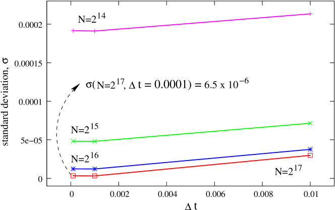
Figure 3: The dependence of the error of the polysymplectic integrator from $\Delta t$ for different values of $\Delta x$.

The results of the polysymplectic integration for different values of $\Delta t$ and $\Delta x=X_{max}/N$ ($X_{max}=400$) are shown of Fig. 3. As expected, the error decreases with $\Delta x$ and $\Delta t$ decreasing. The polysymplectic method appears to be more effective than the pseudo-spectral method. For example, for $N=2^{17}$ and $\Delta t=0.0001$ the error of the polysymplectic scheme $\sigma\approx 6.5\times 10^{-6}$, while for the pseudo-spectral method $\sigma\approx 7\times 10^{-5}$. The CPU time required by the polysymplectic methods is 40000 sec, while the pseudo-spectral method requires $\approx 100000$ sec (on 3GHz Pentium 4 PC).

In conclusion, we have used the polysymplectic formulation of SPE in order to construct the geometric polysymplectic integrator of SPE. We have compared the effectiveness of the corresponding numerical scheme with the pseudo-spectral method which uses the Runge-Kutta integration. The polysymplectic integration appears to be an order of magnitude more precise and approximately 2.5 times faster at long propagation times than the pseudo-spectral method. A comparison with the exact solution of SPE shows that the polysymplectic integrator is more stable and robust than other schemes, and also preserves the energy functional.

References

- [1] M.J. Gotay, J. Isenberg, J.E. Marsden, R. Montgomery, Momentum Maps and Classical Relativistic Fields. Part I: Covariant Field Theory, physics/9801019; Part II: Canonical Analysis of Field Theories, math-ph/0411032.
- [2] G. Giachetta, L. Mangiarotti and G. Sardanashvily, New Lagrangian and Hamiltonian Methods in Field Theory, World Scientific, Singapore 1997.
- [3] O. Krupkova, Hamiltonian field theory, J. Geom. Phys. 43 (2002) 93-132.
- [4] M. de León, M. McLean, L. K. Norris, A. Rey-Roca, M. Salgado, Geometric structures in field theory, math-ph/0208036.
- [5] A. Echeverria-Enriquez, M. de León, M. C. Munoz-Lecanda and N. Roman-Roy, Hamiltonian systems in multisymplectic field theories, arXiv:math-ph/0506003.
- [6] M. Forger, C. Paufler, H. Römer, Hamiltonian multivector fields and poisson forms in multisymplectic field theory, J. Math. Phys. 46 (2005) 112901, math-ph/0407057.
- [7] M. Francaviglia, M. Palese and E. Winterroth, A new geometric proposal for the Hamiltonian description of classical field theories, math-ph/0311018.
- [8] N. Roman-Roy, A. M. Rey, M. Salgado and S. Vilarino, On the k-Symplectic, k-Cosymplectic and Multisymplectic Formalisms of Classical Field Theories, arXiv:0705.4364 [math-ph].
- [9] I.V. Kanatchikov, Canonical structure of classical field theory in the polymomentum phase space, Rep. Math. Phys. 41 (1998) 49-90, hep-th/9709229.
- [10] I.V. Kanatchikov, De Donder-Weyl theory and a hypercomplex extension of quantum mechanics to field theory, Rep. Math. Phys. 43 (1999) 157-70, hep-th/9810165.
- [11] I.V. Kanatchikov, Precanonical quantum gravity: quantization without the space-time decomposition, Int. J. Theor. Phys. 40 (2001) 1121-49, gr-qc/0012074.
- [12] I.V. Kanatchikov, Geometric (pre)quantization in the polysymplectic approach to field theory, hep-th/0112263.
- [13] I.V. Kanatchikov, Precanonical quantization of Yang-Mills fields and the functional Schroedinger representation, Rep. Math. Phys. 53 (2004) 181-193, hep-th/0301001.
- [14] J. E. Marsden, G. W. Patrick, S. Shkoller, Multisymplectic geometry, variational integrators, and nonlinear PDEs, Comm. Math. Phys. 199 (1998) 351-395, math/9807080.
- [15] T.J. Bridges, Multi-symplectic structures and wave propagation, Math. Proc. Camb. Phil. Soc. 121 (1997) 147-190.
- [16] T. Schäfer and C.E. Wayne, Propagation of ultra-short optical pulses in cubic nonlinear media, Physica D 196 (2004) 90-105.
- [17] Y. Chung, C.K.R.T. Jones, T. Schäfer and C.E. Wayne, Ultra-short pulses in linear and nonlinear media, Nonlinearity 18 (2005) 1351-74, nlin.SI/0408020.
- [18] A. Sakovich and S. Sakovich, The short pulse equation is integrable, J. Phys. Soc. Japan 74 (2005) 239-241, nlin.SI/0409034.
-
[19]
J.C. Brunelli,
The short pulse hierarchy,
J. Math. Phys. 46 (2005) 123507, nlin.SI/0601015;
J.C. Brunelli, The bi-Hamiltonian structure of the short pulse equation, Phys. Lett. A 353 (2006) 475-478, nlin.SI/0601014. - [20] A. Sakovich and S. Sakovich, Solitary wave solutions of the short pulse equation, nlin.SI/0601019.
- [21] M. Pietrzyk, I. Kanattšikov, U. Bandelow, On the propagation of vector ultra-short pulses, WIAS preprint No. 128 (2006).
- [22] B. Fornberg, A practical guide to pseudospectral methods, Cambridge University Press, Cambridge, 1998.
- [23] I.V. Kanatchikov, On the Duffin-Kemmer-Petiau Formulation of the Covariant Hamiltonian Dynamics in Field Theory, Rept. Math. Phys. 46 (2000) 107-112, hep-th/9911175.
- [24] T.J. Bridges and S. Reich, Multi-symplectic integrators: numerical schemes for Hamiltonian PDEs that conserve symplecticity, Phys. Lett. A 284 (2001) 184-193.
- [25] P.F. Zhao and M.Z. Qin, Multisymplectic Preissmann scheme for the KdV equation, J. Phys. A 33 (2000) 3613-3626.
-
[26]
J.B. Chen, H.Y. Guo and K. Wu,
Total variation in Hamiltonian formalism and symplectic-energy integrators,
J. Math. Phys. 44 (2003) 1688-1702;
J.B. Chen, Multisymplectic geometry, local conservation laws and a multisymplectic integrator for the Zakharov-Kuznetsov equation, Lett. Math. Phys. 61 (2002) 63-73. - [27] J. Frank, Conservation of wave action under multisymplectic discretizations J. Phys. A 39 (2006) 5479-5493.
- [28] B.E Moore and S. Reich, Multi-symplectic integration methods for Hamiltonian PDEs, Future Generation Computer Systems 19 (2003) 395-402.