Giorgio Sabetta, Emma Perracchione and Ezio Venturino

Department of Mathematics ”G. Peano”, University of Turin - Italy

Abstract. A three population system with a top predator population, i.e. the herbivores, and two prey populations, grass and trees, is considered to model the interaction of herbivores with natural resources. We apply the model for four natural mountain parks in Northern Italy, three located in the Eastern Alps, two of which in the Dolomites and one in the Julian Alps, and one in the Maritime Alps, Northwest Italy. The simulations, based on actual data gathered from contacts with rangers and parks administrators, field samplings and published material, provide useful information on the behavior of the vegetation-wild herbivores interactions and the possible medium-long term evolution of these ecosystems. At the same time they show that these ecosystems are in a very delicate situation, for which the animal populations could become extinguished in case of adverse environmental conditions. The determination of the so-called sensitivity surfaces support our findings and indicate some possible preventive measures to the park admistrators.

1 Introduction

The management of wild parks poses difficult questions to the administrators. The mutual relationships that arise between the various animal and vegetation populations living in them constitute a very complex network of interactions. To intervene in such situations by trying to modify one or some of the parameter values related to these interactions may lead to consequences that are hard to assess and might even be the opposite of the desired outcomes.

In this paper we use a previously built dynamical system model for the interaction of one top predator, here identified as the herbivores population, and two prey, namely the grass and the trees, to study the evolution in the medium term of a few recently created natural parks in Northern Italy, [12].

In spite of the fact that the first models of this kind were built in order to assess the damages that the vegetation, in particular the trees, suffer from overexploitation by the herbivores, [13], the outcome of this investigation points out that, in reality and quite surprisingly, it is the herbivore population that at present is the most endangered one, especially in view of the assumption made in the modelling process. Indeed, we have deliberately excluded possible further negative effects on the herbivores due to their natural predators. This assumption should probably be removed in further studies, as wolves apparently begin to populate at least part of the Western Alps, [2], while as mentioned later on, even the bears have reappeared in the Eastern Alps. But introducing the predators will most likely only worsen the present situation. To assess the herbivores population risk of extinction, we carry out a sensitivity analysis on the model parameters. Moreover, we reconstruct numerically the sensitivity surfaces which enable us to suggest some measures in order to possibly prevent extinction.

The paper is organized as follows. In the next Section, for easiness of the reader, we briefly outline the model already introduced in [12, 13]. Section 3 contains the analysis of the four parks taken in consideration, namely: the Dolomiti Bellunesi Park, the Dolomiti Friulane Park, the Alpi Marittime Park and finally the Prealpi Giulie Park. Section 4 contains several considerations about the sensitivity surfaces and in the final Section we discuss these whole ecosystems survival possibilities at the coexistence level, i.e. with all the population thriving.

2 Background on the Model

For the benefit of the reader we recall here the model introduced in [12] that will be used in the subsequent sections for the analysis of the various specific situations and its main features.

Let $H$, $G$ and $T$ represent respectively the herbivores, grass and trees populations of the environment in consideration. Apart from the obvious ecological fact that the two types of vegetation are different, in that grass grows fast but has a low carrying capacity for surface unit, while trees grow slowly but they contain a large biomass, the reason for considering trees in this context is due to the phenomenon of debarking, that occurs especially when resources are scarce. In such situation, herbivores searching for alternative food tend to bite off stripes of barks from the trees. They thus interrupt the canals that from the roots go up to the leaves to take there the nutrients absorbed from the ground. In this way they damage the tree, sensibly diminishing the clorophyll production up to totally preventing it from occurring. This in due time leads to the tree death.

The model, [12, 13], is a classical predator with two prey system, in which the resources are consumed following a concave response function, usually called the Beddington-De Angelis function, [1, 5]. It has the feature of expressing somewhat the concept of feeding switching, [14, 15, 8, 9, 10], for which herbivores, as stated above, turn to the second resource when the main one is scarce. The Beddington-De Angelis function prevents the herbivores from consuming more than the available amount of grass even if their population becomes very large. Similarly if there is a huge amount of grass the per capita quantity eaten by the herbivores cannot exceed their per capita maximal consumption, $\alpha^{-1}$. Similarly, $\beta$ is the inverse of the herbivores maximal consumption of trees. Letting $r_{1}$ and $r_{2}$ denote the grass and trees growth rates and $K_{1}$ and $K_{2}$ their respective carrying capacities, $\mu$ the metabolic rate of herbivores, $c$ and $g$ the half saturation constants, $e\leq 1$ and $f\leq 1$ the conversion factors of food into new herbivores biomass and $a$ and $b$ the daily feeding rates due to grass and tress, respectively, the model thus reads as follows

$$\dot{H} =-\mu H+ae\frac{H\ G}{c+H+\alpha\ G}+bf\frac{H\ T}{g+H+\beta\ T+\alpha\ G}$$ (1)

$$\dot{G} =r_{1}G\left(1-\frac{G}{K_{1}}\right)-a\frac{H\ G}{c+H+\alpha G}$$

$$\dot{T} =r_{2}T\left(1-\frac{T}{K_{2}}\right)-b\frac{H\ T}{g+H+\beta\ T+\alpha\ G}.$$

All parameters are nonnegative. $K_{1}$, $K_{2}$, $c$ and $g$ are measured in biomass, $e\leq 1$, $f\leq 1$, $\alpha$ and $\beta$ are pure numbers, $\mu$, $r_{1}$, $r_{2}$, $a$ and $b$ are rates.

This model has a few equilibria. Coexistence can only be assessed via numerical simulations, in view of the high nonlinearities appearing in (1). The origin is always unstable, preventing ecosystem collapse. Of the remaining possible equilibria, we mention here only the herbivore-free point $E_{3}=(0,K_{1},K_{2})$ and the forest-free equilibrium $E_{4}=(H_{4},G_{4},0)$ because they play a role also in this investigation. In fact, the stability of equilibrium with loss of woods, representing a severe damage for the environment, motivated the earlier investigations [12, 13]. Here we will need their feasibility and stability conditions given by, [12, 13]: stability of $E_{3}$

$$ae\dfrac{K_{1}}{c+\alpha\ K_{1}}+bf\dfrac{K_{2}}{g+\alpha\ K_{1}+\beta\ K_{2}}<\mu~{};$$ (2)

feasibility of $E_{4}$

$$G_{4}>\dfrac{c\mu}{ae-\mu\alpha}~{};$$ (3)

stability of $E_{4}$:

$$r_{2}\left(g+H_{4}+\alpha\ G_{4}\right)<H_{4}~{}.$$ (4)

3 Parameter estimation and simulations

In this Section we discuss the parameters that are common to all parks. The remaining parameters, namely the carrying capacities $K_{1}$ and $K_{2}$ and the grass and trees half saturation constants $c$ and $g$, are park-dependent and will be discussed in next subsections.

To estimate the parameters we refer to [7, 12, 13]. Specifically, in [7] tables providing estimation of the annual net primary production of several environments are shown. The latter allow to estimate the growth rates of grass and trees, that in all the considered natural parks are about $r_{1}=0.01$ and $r_{2}=0.0006$. In such estimate we take into account that the growth period of grass and trees can be estimated to be about $120$ days every year.

To set the parameter $\mu=0.03$ we refer to [12]. It means that an herbivore with no food available dies in about $30$ days. This is consistent with similar mammals not accustomed to a lethargic period.

The parameter $\alpha$, i.e. the inverse of the per capita maximal consumption of grass, can be approximated as a percentage of the herbivore itself; this percentage is about $4\%-5.5\%$, [13]. In the following we fix $\alpha=0.05^{-1}$. Even if the parameter $\beta$ is the analogous of $\alpha$ for trees, its estimation is different. In fact when an herbivore switches its attention to a tree it may cause the death of the whole tree even if it takes a small piece of barks. In [13], in case of sheep, $\beta$ is estimated to be $1$. However the tree death in case of our herbivores does not occur with likelihood higher than the one due to sheep because a wild herbivore peels off vertical stripes of bark (and not circular stripes of barks at the bottom of the tree). This difference implies that the communication between roots and leaves is not totally interrupted. As a consequence, remarking that $\beta$ is the inverse of the per capita maximal consumption of trees by herbivores, we set $\beta=8$.

We remark that $e$ and $f$ are the herbivores assimilation coefficients of grass and trees, respectively. Since grass represents the preferred resource and moreover herbivores can survive by eating grass alone, it means that an adequate amount of grass can satisfy the metabolic needs of herbivores, i.e. $e>>f$. Similarly, taking into account the above consideration $a>>b$ must hold. In the following we set $e=0.605$, $f=0.001$, $a=0.98$ and $b=0.002$ as reference values.

In our simulations all the above parameters have a fixed value, since they are about the same in each park.

A common remark for the subsequent analysis is the fact that the whole ecosystems dynamics is analysed in the absence of wolf and other herbivores predators and of possible human activities and interferences.

Further, the herbivores-free equilibrium $E_{3}$ in all parks is unstable. The left-hand side of (2) has indeed the values $0.0302$ for the Dolomiti Bellunesi Park and for the Dolomiti Friulane Park, and $0.0301$ for the Alpi Marittime and the Prealpi Giulie, while the right hand side is always $\mu=0.03$. The equilibrium $E_{4}$ stating the extinction of the forests is feasible in all the parks. In fact the right-hand side of (3) and the minimum of $G_{4}$ in two centuries have respectively the values $6.78\times 10^{5}$ and $1.83\times 10^{6}$ for the Dolomiti Bellunesi, $1.05\times 10^{6}$ and $2.52\times 10^{6}$ for the Dolomiti Friulane, $4.63\times 10^{5}$ and $1.19\times 10^{6}$ for the Alpi Marittime, $1.56\times 10^{5}$ and $3.43\times 10^{5}$ for the Prealpi Giulie parks. However $E_{4}$ is never stable, condition (4) is not verified. For each case we find indeed the following values of the left and right hand sides of (4): Dolomiti Bellunesi: $6.9\times 10^{5}$ and $3.2\times 10^{5}$; Dolomiti Friulane: $5.2\times 10^{5}$ and $2.7\times 10^{5}$; Alpi Marittime: $2.9\times 10^{5}$ and $2.1\times 10^{5}$; Prealpi Giulie: $1.13\times 10^{5}$ and $8.7\times 10^{4}$. Nevertheless, we will see later in assessing the sensitivity surface that in spite of these results, the possibility of herbivores extinction is real. No other equilibrium exists at a stable level with one or more vanishing populations.

3.1 Dolomiti Bellunesi National Park

The Dolomiti Bellunesi National Park was established in 1990. It is located in the Veneto Region (NE Italy) in the territory of 15 municipalities, with a surface of about $32000$ ha. of which $8000$ ha. of grass and about $19000$ of forests; in the remaining part there are rivers, lake, pastures and rocks, which are excluded from our study. About $16000$ ha. comprise 8 naturals reserves belonging to the biogenetic reserve of the Council of Europe. The territory includes medium and high mountain areas with altitudes between 400 and 2565 meters above sea level, the highest peak being the Schiara mountain.

There are some protected areas near the park that contribute to construct a large biogeographic network. The park includes a great environmental variety, allowing many animal species to find suitable living and reproducing conditions. Nowadays the park harbors about 115 birds species, 20 amphibian and reptile species, about 100 butterfly species and 50 beetle species. Here some insect species are present that are found nowhere else in the world.

In this park there is a relevant herbivore population. Several species are present, estimated by the park rangers, among which about 3000 chamois (Rupicapra rupicapra), whose average weight is about 50 Kg., about 2000 roes (Capreolus capreolus), their average weight being around 25 Kg., 250 mouflons (Ovis aries), with an average weight of 35 Kg. and 300 deers (Cervus elaphus), each one on average weighting about 200 Kg. These last species occupy the most elevated areas. They exhibit seasonal migrations, climbing upwards in the summer and descending in the valley during the winter.

Let us recall here that the biomass unit is given in tons for all the model populations, the hectares given in the Tables for measuring the amount of grass and trees are suitably converted into biomass tons. On the basis of the above data and following [7] for the conversions, we find the carrying capacities and the half saturation constants to be $K_{1}={3469640.64}$, $K_{2}={15695993.39}$, $c={101862.16}$ and $g={1001229580.18}$. We set the initial conditions using the rangers data and the park vegetation distribution:

$$H(0)=268.750\qquad G(0)={2313093.76}\qquad T(0)={1046399.56}.$$ (5)

We ran our Matlab code to assess the system’s behavior in the medium term timespan. Our simulations show that under undisturbed conditions, the system could reach a stable coexistence equilibrium in about 150 years.

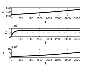
Figure 1: Dolomiti Bellunesi’s system evolution over ten years with initial conditions set as in Equation (5).

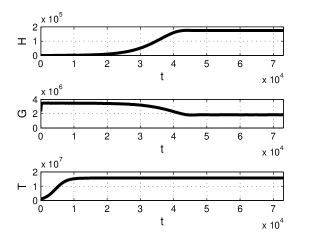
Figure 2: Dolomiti Bellunesi’s system evolution over two centuries with initial conditions set as in Equation (5).

There is a continuous increase of the herbivores population until they reach the equilibrium where they become $647.44$ times the initial condition. Due to a initial slow increase of herbivores, the grass population has a fast initial increase. After that, when herbivores grows a little faster, the grass population starts to decrease until the equilibrium where it becomes about the $79\%$ of the initial condition. The trees population has as imilar behavior. The latter has an initial growth, a little slower than the grass population. After that, it stabilizes at the equilibrium. See Figure 1 for the short range and Figure 2 for the medium-long term.

3.2 Dolomiti Friulane Natural Park

The park, established in 1996, is inserted in the mountains above the high plains of the Friuli-Venezia Giulia region (NE Italy).

The territory has high geological, environmental and natural interest, with a high degree of wilderness, particularly evident due to the absence of many communication roads. Three major tectonic lines are present in this area. The widespread presence, up to several thousands of years ago, of ancient glaciers characterized its geomorphological aspect. In much more recent times, we recall the 1963 catastrophe due to the great landslide of Monte Toc into the artificial lake of Vajont. It constitutes a unique example of colossal landslide.

The park extends for $37275.49$ hectares, its composition is shown in Table 1, the acronym CLC code stands for the CORINE-Land Cover code.

CLC	Denomination	Area	%
code		(ha)
122	Railways, roads and technical infrastructures	$1.07$	$0.003\%$
131	Mining areas	$2.56$	$0.01\%$
3113	Mixed forest of broad-leaf	$576.01$	$1.5\%$
	(Fraxinus, Orno-ostrietum)
3115	Beech forest (Fagus sylvatica L.)	$9247.13$	$24.8\%$
3122	Pine forest (Pinus nigra, Pinus nigra laricio,	$2751.61$	$7.4\%$
	Pinus sylvestris, Pinus Heldreichii)
3123	Fir forest (Picea abies, Abies alba)	$2020.34$	$5.4\%$
3124	Larch (Larix) and pine (Pinus cembra) forest	$474.02$	$1.3\%$
3131	Conifers and broad-leaf forest	$2957.55$	$7.9\%$
3211	Continuous meadows	$2931.26$	$7.9\%$
3212	Discontinuous meadows	$891.00$	$2.4\%$
322	Moorland and bushed land	$8370.44$	$22.5\%$
332	Rocks	$3367.80$	$9.0\%$
333	Thin vegetation areas	$3060.52$	$8.2\%$
411	Internal swamp	$1.77$	$0.005\%$
511	Rivers, drains and waterways	$474.99$	$1.3\%$
512	Ponds	$147.42$	$0.4\%$
	Total	$37275.49$	$100\%$

Table 1: Dolomiti Friulane Natural Park environmental composition.

The park can be regarded as wild, as there are no pastures due to the poor anthropization, a further sign of this fact being the presence of the golden eagle. There are about 2500 chamois (Rupicapra rupicapra), 300 deer (Cervus elaphus), 800 roes (Capreolus capreolus) and a large herd of rock goat (Capra ibex), with an average weight of about 85 Kg. The latter population consists nowadays of at least 196 individuals versus the 239 of 2008, but in spite of this it presently appears to be in expansion, due to an increase of the colonization and an increase of reproductive capabilities. In the last three years an increase of about $10\%$ in the population of chamois (Rupicapra rupicapra) has been observed, probably as a rebound with respect to the decrease of the previous years: $2586$ individuals in 2006, $2476$ in 2007 and $2373$ in 2008.

For the simulations we use the following parameters based on the data above: $K_{1}={4385112.18}$, $K_{2}={10464154.82}$, $c={155246.86}$ and $g={804938520.99}$, with initial conditions:

$$H_{0}=221.660\qquad G_{0}={2923408.12}\qquad T_{0}={6976103.21}.$$ (6)

Again, from our simulation we observe that the herbivores population grows until the equilibrium is reached in about 150 years, see Figure 3. There herbivores attain a value which is about $965$ times the initial condition. Grass and trees populations have a faster growth in the first period, due to a slow growth of the herbivores population. After this period, grass and trees populations reach the equilibrium. Specifically, after an initial surge, grass population decreases until the equilibrium becoming $85\%$ of the initial condition.

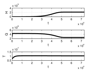
Figure 3: Dolomiti Friulane’s system evolution over two centuries with initial conditions set as in Equation (6).

3.3 Alpi Marittime Natural Park

This park was established only in 2009. It is located in the south-west part of Piedmont region, NW Italy. The territory extends for about $19751.23$ ha. subdivided as shown in Table 2.

According to a 2012 survey, in this park live about 3828 chamois (Rupicapra rupicapra), and 591 rock goats (Capra ibex), this datum going back to a census of the year 2003. Also a few individuals of roes (Capreolus capreolus), deer (Cervus elaphus) and mouflons (Ovis aries), have been spotted, but never accurately surveyed. In absence of better data, to account for their contributions too, in our simulations we arbitrarily set their overall population at $100$ individuals with an average weight of about $85$ kilograms.

Denomination	Area (ha)
Fir forest (Abies alba, Picea abies)	$170.48$
Mixed forests (Acer, Fraxinus, Tilia)	$277.55$
Bushes	$626.60$
Pioneer and invasion woodlands (Populus, Betula, Corylus avellana)	$429.05$
Chestnut forest Castanea Sativa Miller	$42.42$
Fagus sylvatica L.	$5099.38$
Larch (Larix) and pine (Pinus cembra) forest	$1088.48$
Shrubbery	$1522.21$
Meadows	$2011.35$
Pines forest (Pinus mugo)	$3082.2$
Rocked meadows	$6042.34$
Pastures	$1309.4$
Oak forests (Quercus petraea, Quercus pubescens)	$988.30$
Reafforestation	$864.60$
Total	$19751.230$

Table 2: Alpi Marittime Natural Park environmental composition.

In this situation, the carrying capacities and the half saturation constants turn out to have the following values: $K_{1}={2184427.67}$, $K_{2}={5720905.98}$, $c={69587.52}$ and $g={395981556.29}$. Moreover we set the next initial conditions as follows:

$$H_{0}=209.635\qquad G_{0}={1456285.16}\qquad T_{0}={3813937.32}.$$ (7)

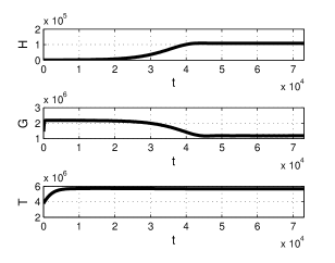
Figure 4: Alpi Marittime’s system evolution over two centuries with initial conditions set as in Equation (7).

The pattern already discovered of a initial fast growth of grass and trees populations matched by a corresponding slow increase of the herbivores population in the first period occurs here as well. After this period again we have a faster growth of the herbivores and consequently their stabilization at the equilibrium. At the same time we have a decrease of grass until the equilibrium, where the herbivores are about $519$ times the initial condition and grass is about the $81\%$ the initial condition.

3.4 Prealpi Giulie Natural Park

This park was established in 1996 in the Friuli-Venezia Giulia region (NE Italy). It is an area of about $10000$ ha., specific because in it the Mediterranean, the Illyrian and the Alpine biogeographic regions come in contact. Their characteristics combine to form an ecosystem with extraordinary biodiversity. The composition of the park is given in Table 3.

Denomination	Area (ha)
Meadows	$1691.15$
Evolving forests	$722.53$
Thin vegetation areas	$723.94$
Agricultural fields	$23.63$
Conifer forests	$218.65$
Broad-leaf forests	$3186.00$
Mixed forests	$1885.60$
Moorland and bushed land	$157.43$
Rocks and cliff	$795.98$
Sands	$30.48$
Total	$9435.40$

Table 3: Prealpi Giulie Natural Park environmental composition.

In the park wildlife species of southern, Mediterranean, and Eastern European origin thrive. In recent years even the presence of the brown bear and of the lynx has been established. About 100 species of birds have been observed, among them there are several predators (eagle owl, tawny owl, boreal owl, golden eagle). As for the herbivores population, at present it is composed of about 30 deer (Cervus elaphus), 257 ibex (Capra ibex) and of chamois (Rupicapra rupicapra). The chamois population had the following evolution: 227 individuals in 2008, 249 in 2009, 153 in 2010, with a rebound to 383 in 2011 and 492 in 2012. From this and using Table 3, in the simulations we employ the following values: $K_{1}={576651.52}$, $K_{2}={3572655.97}$, $c={23537.55}$ and $g={316851220.79}$ and initial conditions:

$$H_{0}=52.445\qquad G_{0}={384434.35}\qquad T_{0}={6012.78}.$$ (8)

The system qualitatively behaves similarly to the former ones.

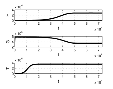
Figure 5: The Prealpi Giulie system evolution over two centuries with initial conditions set as in Equation (8).

4 Approximation of sensitivity surfaces

The results of several numerical experiments indicate that the parameters most affecting the system’s final configuration are $\mu$, $e$ and $\alpha$. In particular the herbivores’ population level appears to be very sensitive and under the threat of a high risk of extinction. In Figure 6 left, the surface shows the value attained by the herbivores as function of the parameters $\mu$ and $e$ after $4$ years. The surface has been reconstructed with state-of-the-art techniques, [3, 4]. The dot represents the situation in the present ecosystem conditions. The right frame shows that it is very close to the line beyond which the herbivores population would vanish. Thus, under possible ecosystem parameter changes, induced for instance by climatic variations or random environmental disturbances, the present situation has some potential risks for an evolution toward an extinction of the herbivores population in the short time span.

In the three-dimensional parameter space $(\mu,e,\alpha)$ Figure 7 represents instead the separatrix of the basins of attraction of the coexistenc equilibrium $E^{*}$ and of the herbivores-free equilibrium $E_{3}$. Again the actual value of the herbivores population, represented by the dot, is very close to this surface, although at present beloging to the not endangered region. But clearly changes in the environmental conditions that might lead even to relatively small parameter perturbations may well push it into the region where the herbivores would be doomed.

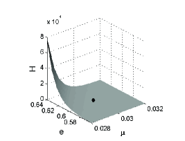
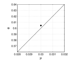
Figure 6: Dolomiti Bellunesi’s system. Left frame: the surface represents the equilibrium value of the herbivores as function of the parameters $\mu$ and $e$ at the end of 4 years. Note that the surface flattens onto the horizontal coordinate plane; Right frame: the curve separates the region in which the surface has a nonzero level, top left, from the region in which the herbivores population vanishes, bottom right. The dot represents the herbivores population level in the present conditions of the ecosystem. Its closeness to the range in which it would vanish is evident.

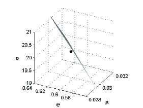
Figure 7: Dolomiti Bellunesi’s system. In the parameter space $(\mu,e,\alpha)$ we show the surface separating the basins of attraction of the coexistence equilibrium $E^{*}$, bottom left, from the one of the herbivore-free equilibrium $E_{3}$, top right. The dot represents the actual situation. Again, small parameter variations may push it into the other basin of attraction, thereby entailing the herbivores extinction.

5 A Caveat on the Ecosystems Preservation

Qualitatively, all the simulations performed in Section 3, by estimating the parameters with techniques which are widely used in literature [7, 12], show very similar results for all the four ecosystems in consideration. But note that the results obtained for the Dolomiti Friulane Natural Park and for the Dolomiti Bellunesi National Park are very similar also from the quantitative point of view. This remark could be attributed to the similar extension and to the similar initial erbivores biomass. It is likely that by considering wolves and other herbivores predators, as well as possible human intervention, the results might differ somewhat.

Assessing and comparing more closely all the simulations results shown in Section 3 it is to be further remarked that in all these ecosystems there seems no immediate high risk of extinction for the herbivores in the actual situation. This result is substantiated by the equilibrium analysis. While for coexistence we have to rely only on simulations, for the herbivores-free equilibrium $E_{3}=(0,K_{1},K_{2})$ we have the stability conditions explicitly, (2). As stated in Section 3 above, the equilibrium is not stable. Moreover we can also exclude any other bistability cases. Excluding bistability situations implies also that the equilibrium with no forests $E_{4}$ is always unstable. This is consistent with the fact that, differently from the context of sheep [12], the trees damage due to wild herbivores is less significant than the one due to sheep.

Therefore, from this analysis there seems to be no risk of extinction for herbivores in the present conditions. On the other hand, in Section 4 we pointed out that the system is really sensitive with respect to small perturbations of several parameters and such perturbations can instead lead to the extinction. By reconstructing the sensitivity curves and surfaces we can deduce that the system (1) is really sensitive with respect to the parameters $\mu$, $e$ and $\alpha$. Specifically, for small perturbations of such parameters a transcritical bifurcation between the coexistence equilibrium point and the herbivores-free equilibrium occurs. Furthermore, since from the estimation of parameters the current ecosystem state is really close to the separatrix a small perturbation can drive the ecosystem into the region where herbivores extinction occurs.

In order to possibly prevent the ecosystem to fall into the unwanted region the strategy is therefore to move away from the separatrix surface. Specifically, from a mathematical point of view, a decrease of $\mu$ and $\alpha$, combined with an increase of $e$, leads to a benefit for the population $H$. We can try to directly act on $\mu$ and $\alpha$. Recalling that $\mu$ is the mortality rate, building safety niches during winter for instance surely leads to a decrease of the herbivores mortality rate. Moreover, by planting grass more nutritious than the existing one and/or by using fertilizers we can try to increase the nutrient assimilation coming from grass, leading to an increase of $\alpha^{-1}$. In this way, mathematically speaking, in order to prevent extinction in the $\mu-e-\alpha$ parameter space we move away the ecosystem state from the separatrix.

References

- [1] J. Beddington, J.Anim. Ecol. 51, 331 (1975).
- [2] M. Borgia, Luna Nuova, Avigliana, Italy, 2003.
- [3] R. Cavoretto, S. Chaudhuri, A. De Rossi, E. Menduni, F. Moretti, M. C. Rodi, E. Venturino, Numerical Analysis and Applied Mathematics ICNAAM 2011, T. Simos, G. Psihoyios, Ch. Tsitouras, Z. Anastassi (Editors), AIP Conf. Proc. 1389, 1220 (2011); doi: 10.1063/1.3637836.
- [4] R. Cavoretto, A. De Rossi, E. Perracchione, E. Venturino, International Journal of Computer Mathematics, to appear (2015).
- [5] D. De Angelis, R. Goldstein, R. O’Neill, Ecol. 56, 881 (1975).
- [6] G. E. Fasshauer, Meshfree Approximations Methods with Matlab, World Scientific Publishers Co., Inc., River Edge, NJ (2007).
- [7] T. Fujimori, Ecological and Silvicultural Strategies for Sustainable Forest Managment, Elsevier - Amterdam, Nederland (2001).
- [8] Q.J.A. Khan, E.V. Krishnan, M.A. Al-Lawatia, Z. Angew. Math. Mech. 82, 125 (2002).
- [9] Q. J. A. Khan, E. Balakrishnan, G. C. Wake, Bull. Math. Biol. 66, 109 (2004).
- [10] S. Palomino Bean, A. C. S. Vilcarromero, J. F. R. Fernandes, O. Bonato, TEMA Tend. Mat. Apl. Comput. 7, 317 (2006).
- [11] G. Pulina, R. Bencini, Dairy Sheep Nutrition, CABI Publishing, Cambridge MA, USA (2004).
- [12] L. Tamburino, E. Venturino, Int. J. Comp. Math. 89, 1808 (2012).
- [13] L. Tamburino, V. La Morgia, E. Venturino, Computational Ecology and Software 2, 26 (2012).
- [14] M. Tanksy, J. Theor. Biol. 70, 263 (1978).
- [15] A. C. S. Vilcarromero, S. Palomino Bean, J. F. R. Fernandes, O. Bonato, Proceedings Of Congreso Latino Americano de Biomatematica (Alab-V Elaem) X, (2001).