Hall conductance of two-band systems in a quantized field

Abstract

Kubo formula gives a linear response of a quantum system to external fields, which are classical and weak with respect to the energy of the system. In this work, we take the quantum nature of the external field into account, and define a Hall conductance to characterize the linear response of a two-band system to the quantized field. The theory is then applied to topological insulators. Comparisons with the traditional Hall conductance are presented and discussed.

I Introduction

The integer quantum Hall effect(IQHE) is manifested by a remarkably precise quantization of the transverse conductance in two-dimensional electron systems in presence of a strong perpendicular magnetic field. Its discoveryklitzing80 ; tsui82 has had profound implications for the understanding of matter, and it may find potential applications in quantum information processingsimon08 . The integer quantum Hall effects can be understood in the single particle frameworkhasan10 ; qi10 : Charged particles in a magnetic field form Landau levels with energy splitting that is proportional to the strength of the magnetic field, and when an integer number of Landau levels are filled, the Hall conductance is quantized and characterized by the TKNN numberthouless82 that is now treated as a topological invariant called Chern number . This topological understanding of the IQHE is a remarkable step of progress, opening up the field of topological electronic states in condensed matter physics. Later, Haldanehaldane88 found that a periodic 2D honeycomb lattice without net magnetic flux can in principle support a similar integer quantum Hall effect. This result suggested that certain materials, other than the 2D electron gas under magnetic field, can have topologically non-trivial electronic band structures, which can be characterized by a non-zero Chern number. Such materials are called topological insulators now.

In contrast to ordinary band insulators, topological insulatorkonig07 ; roth09 ; qi11 comes with gapless chiral edge states that each carries a quantum of conductance, $\frac{e^{2}}{h}$. The number of edge states is mathematically given by the value of the topological invariant, namely the Chern number, that can only assume integer values similar to winding numbers. The integer nature of the Chern number is what makes the edge states, and hence the quantization of the conductivity.

Physically, the quantized conductance can be derived by linear response theory. In the context of quantum statistics, the exposition of the linear response theory can be found in the paper by Ryogo Kubokubo57 , which defines particularly the Kubo formula. This formula gives a linear response of quantum systems to external classical fields. Particularly, it considers the response to a classically electric filed of an otherwise stationary observable, say current. The goal for us in this work is to answer the following question: When the field is quantized, how a quantum system responses to that field?

The answer to this question is not trivial. Firstly, this answer conceptually contributes to the broader question of how quantum systems respond to a quantized driving. A simple setting is provided by a two-band model (that can describe TIs) driven by a single mode electromagnetic field with frequency $\omega$, with the Hall current denoting the response to the driving. Secondly, the answer extends the theory of adiabatic response of quantum systems undergoing unitary evolutionthouless83 ; berry93 to bipartite quantum systems consisting of a quantum system and a quantum driving field kibis10 ; dora12 ; trif12 ; gulasci15 . As a result, the presented formalism opens a remarkable new area for response theory, where condensed matter physics and quantum optics meet.

II formalism

As a starting point, let us consider a generic two-band Hamiltonian,

$$H_{0}(\vec{k})=\vec{d}(\vec{k})\cdot\vec{\sigma}+\epsilon(\vec{k})\cdot\textbf{I},$$ (1)

where I is the $2\times 2$ identity matrix, $\vec{\sigma}=(\sigma_{x},\sigma_{y},\sigma_{z})$ are Pauli matrices, $\epsilon(\vec{k})$ and $\vec{d}(\vec{k})$ depend on the materials under study and determine its band structure. The two bands may describe different physical degrees of freedom. If they are the components of a spin-1/2 electron, $\vec{d}(\vec{k})$ stands for the spin-orbit coupling. If they denote the orbital degrees of freedoms, then $\vec{d}(\vec{k})$ represents the hybridization between bands. The discussion below is completely independent of the physical interpretation of the Hamiltonian Eq. (1), and leads to a general formalism regarding the two-band system.

In the next section, we will specify $\epsilon(\vec{k})$ and $\vec{d}(\vec{k})$ to examine the response of a concrete quantum system to a quantum driving field. In the presence of a electromagnetic field represented by vector potential $\vec{A}$ of frequency $\omega$, by changing the crystal momentum, $\vec{k}\rightarrow(\vec{k}-\frac{e}{\hbar}\vec{A}),$ we can still use the two-band model to describe the system in the field. In the weak field limit, we may expend the Hamiltonian up to the first order in $\vec{A}$,

$$H=H_{0}(\vec{k}-\frac{e}{\hbar}\vec{A})\simeq H_{0}(\vec{k})-\frac{e}{\hbar}\sum_{j=x,y,z}(\nabla d_{j}\cdot\vec{A})\cdot\sigma_{j}.$$ (2)

In the Hilbert space spanned by the eigenstates of $\sigma_{z}$, satisfying $\sigma_{z}|\Uparrow\rangle=+|\Uparrow\rangle,$ $\sigma_{z}|\Downarrow\rangle=-|\Downarrow\rangle,$ the eigenvalues and the corresponding eigenstates of $H_{0}(\vec{k})$ take, $\varepsilon_{\pm}=\epsilon(\vec{k})\pm|\vec{d}|$ and $|\varepsilon_{+}\rangle=\cos\frac{\theta}{2}e^{-i\phi}|\Uparrow\rangle+\sin\frac{\theta}{2}|\Downarrow\rangle$, $|\varepsilon_{-}\rangle=\sin\frac{\theta}{2}e^{-i\phi}|\Uparrow\rangle-\cos\frac{\theta}{2}|\Downarrow\rangle$. Here, $|\vec{d}|=\sqrt{d_{x}^{2}+d_{y}^{2}+d_{z}^{2}}$, $\cos\theta=\frac{d_{z}}{|\vec{d}|}$, and $\tan\phi=\frac{d_{y}}{d_{x}}.$

Taking the field to be in the $x-$direction, $\vec{A}=(A_{x},0,0),$ and decomposing the field in a mean amplitude $\bar{E}$ and a quantum part, $\delta_{E}(a^{\dagger}+a)$, i.e.,

$$A_{x}=E_{x}t=\bar{E}t+\delta_{E}(a^{\dagger}+a)t,$$ (3)

we write the Hamiltonian as,

$$H = |\vec{d}|\tau_{z}+(g_{c}|\varepsilon_{+}\rangle\langle\varepsilon_{-}|e^{i\omega t}+h.c.)$$ (4)

$$+ \left[g_{q}|\varepsilon_{+}\rangle\langle\varepsilon_{-}|(a^{{\dagger}}e^{-i\omega t}+ae^{i\omega t})+h.c.\right].$$

Here $g_{c}\equiv ie\bar{E}\langle\varepsilon_{+}|\frac{\partial\varepsilon_{-}}{\partial k_{x}}\rangle$, $g_{q}\equiv ie\delta_{E}\langle\varepsilon_{+}|\frac{\partial\varepsilon_{-}}{\partial k_{x}}\rangle.$ $\tau_{+}\equiv|\varepsilon_{+}\rangle\langle\varepsilon_{-}|$, $\tau_{-}\equiv\tau_{+}^{\dagger}$, and $\tau_{z}\equiv|\varepsilon_{+}\rangle\langle\varepsilon_{+}|-|\varepsilon_{-}\rangle\langle\varepsilon_{-}|.$ $\bar{E}$ and $\delta_{E}$ are real, $a^{\dagger}$ and $a$ stands for the creation and annihilation operator of the quantum part of the field.

In terms of eigenstates of $H_{c}$ defined by $H_{c}\equiv|\vec{d}|\tau_{z}+(g_{c}|\varepsilon_{+}\rangle\langle\varepsilon_{-}|e^{i\omega t}+h.c.),$ the Hamiltonian can be rewritten as,

$$H=\sum_{j=+,-}E_{j}^{c}|E_{j}^{c}\rangle\langle E_{j}^{c}|+\hbar\omega a^{\dagger}a+\eta(a^{\dagger}+a)|E_{+}^{c}\rangle\langle E_{-}^{c}|+h.c..$$ (5)

Here, $\eta=-g_{q}\cos^{2}\frac{\alpha_{c}}{2}e^{-i\beta_{c}}+g_{q}^{*}\sin^{2}\frac{\alpha_{c}}{2}e^{i\beta_{c}}$, $E_{\pm}^{c}=\pm\sqrt{(|\vec{d}|-\frac{\hbar\omega}{2})^{2}+|g_{c}|^{2}}$, $|E_{+}^{c}\rangle=\cos\frac{\alpha_{c}}{2}e^{i\beta_{c}}|\varepsilon_{+}\rangle+\sin\frac{\alpha_{c}}{2}|\varepsilon_{-}\rangle,$ and $|E_{-}^{c}\rangle=\sin\frac{\alpha_{c}}{2}e^{i\beta_{c}}|\varepsilon_{+}\rangle-\cos\frac{\alpha_{c}}{2}|\varepsilon_{-}\rangle.$ $\cos\alpha_{c}=\frac{2|\vec{d}|-\hbar\omega}{\sqrt{(2|\vec{d}|-\hbar\omega)^{2}+4|g_{c}|^{2}}}$, $\tan\beta_{c}=\Im(g_{c})/\Re(g_{c})$ with $\Im(...)$ and $\Re(...)$ denoting the imaginary and real part of $(...),$ respectively.

Under the rotating-wave approximation(RWA), the eigenstate and the corresponding eigenvalues take,

$$|E_{\pm}^{q}\rangle_{n} = \cos\frac{\alpha_{q}^{\pm}}{2}e^{i\beta_{q}}|E_{+}^{c}\rangle\otimes|n\rangle+\sin\frac{\alpha_{q}^{\pm}}{2}|E_{-}^{c}\rangle\otimes|n+1\rangle,$$ (6)

where $\cos\alpha_{q}^{+}=\frac{\Delta}{\sqrt{\Delta^{2}+4|\eta|^{2}(n+1)}}$, $\alpha_{q}^{-}=\alpha_{q}^{+}-\pi,$ $\tan\beta_{q}=\frac{\Im(\eta)}{\Re(\eta)}$, and $\Delta=2E_{+}^{c}-\hbar\omega.$ $|n\rangle$ denotes a Fock state of the field. The results beyond the RWA will be given in Appendix. Using the relation $v_{y}=\frac{1}{\hbar}\frac{\partial H(\vec{k})}{\partial\vec{k}},$ we easily find $v_{y}=\frac{\hbar k_{y}}{m^{*}}+\sum_{j=x,y,z}\frac{\partial d_{j}}{\hbar\partial k_{y}}\cdot\sigma_{j}.$ Then the $y-$component of the average velocity in state $|E_{-}^{q}\rangle$ is given by,

$$\bar{v}_{y} = {}_{n}\langle E_{-}^{q}|v_{y}|E_{-}^{q}\rangle_{n}$$ (7)

$$= \sin^{2}\frac{\alpha_{q}^{-}}{2}\langle E_{+}^{c}|v_{y}|E_{+}^{c}\rangle+\cos^{2}\frac{\alpha_{q}^{-}}{2}\langle E_{-}^{c}|v_{y}|E_{-}^{c}\rangle$$

$$= -\cos\alpha_{q}^{-}\Re(\sin\alpha_{c}e^{-i\beta_{c}}\langle\varepsilon_{+}|v_{y}|\varepsilon_{-}\rangle).$$

Consider the system under an external electric field $E_{x}\neq 0$ without magnetic field. The dc current density $j(\bar{E},\delta_{E},n)=j_{y}(\bar{E},\delta_{E},n)$ can be then obtained from the equation given above by,

$$j_{y}(\bar{E},\delta_{E},n)=-e\int\frac{dk_{x}dk_{y}}{(2\pi)^{2}}\bar{v}_{y}\big{|}_{\omega\rightarrow 0}.$$ (8)

For the quantum part of the field, a linear response of the system to the photon number in the field is then defined by,

$$\sigma_{n}=\frac{\partial j(\bar{E},\delta_{E},n)}{\partial n}\big{|}_{n\rightarrow 0}.$$ (9)

After some straightforward algebra, and expanding $\sigma_{n}$ up to the first order in $\bar{E}$, we have

$$\sigma_{n}=\frac{e^{2}\bar{E}}{\hbar}\int\frac{idk_{x}dk_{y}}{(2\pi)^{2}}\frac{\partial\cos\alpha_{q}^{-}}{\partial n}\bigg{|}_{n=0}\left[\langle\frac{\partial\varepsilon_{-}}{\partial k_{x}}|\frac{\partial\varepsilon_{-}}{\partial k_{y}}\rangle-\langle\frac{\partial\varepsilon_{-}}{\partial k_{y}}|\frac{\partial\varepsilon_{-}}{\partial k_{x}}\rangle\right].$$ (10)

Noticing that the Berry curvature of the lower bare band $|\varepsilon_{-}\rangle$ is defined by $\Omega^{-}_{xy}(\vec{k})=i\left[\langle\frac{\partial\varepsilon_{-}}{\partial k_{x}}|\frac{\partial\varepsilon_{-}}{\partial k_{y}}\rangle-\langle\frac{\partial\varepsilon_{-}}{\partial k_{y}}|\frac{\partial\varepsilon_{-}}{\partial k_{x}}\rangle\right]$, we find that $\sigma_{n}$ is simply the BZ integral of the Berry curvature weighted by the factor $\frac{\partial\cos\alpha_{q}^{-}}{\partial n}\bigg{|}_{n=0}$. Discussions on Eq. (10) are in order. Consider a limit of $\Delta\gg 4|\eta|^{2}(n+1)$, $\cos\alpha_{q}^{-}\sim\frac{2|\eta|^{2}(n+1)}{\Delta^{2}}-1,$ then $\sigma_{n}\simeq\frac{e^{2}}{h}\bar{E}\frac{2|\eta|^{2}}{\Delta^{2}}C_{n}.$ Here, we assume $\frac{2|\eta|^{2}}{\Delta^{2}}$ independent of $\vec{k},$ and $C_{n}$ denotes the Chern number of band $|\varepsilon_{-}\rangle.$ This suggests that $\sigma_{n}$ behaves like the conventional Hall conductance. In fact, as will be seen below, the response of the two-band system to the photon number in the field witnesses the transition points of the system.

In addition, we may define a response of the topological insulator to the mean amplitude of the field, taking the quantum part of the field into account. Namely, define

$$\sigma_{q}=\frac{\partial j(\bar{E},\delta_{E},n)}{\partial\bar{E}}\bigg{|}_{\bar{E}=0}$$ (11)

to characterize the response of the two-band system to the classical part of the field. Simple algebra shows that, $\sigma_{q}=\frac{e^{2}}{\hbar}\int\frac{dk_{x}dk_{y}}{(2\pi)^{2}}\cos\alpha_{q}^{-}\Omega^{-}_{xy}(\vec{k}).$ A limiting case for $\sigma_{q}$ is that $\sigma_{c}=\sigma_{q}\big{|}_{\delta_{E}=0}=\frac{\partial j(\bar{E},\delta_{E},n)}{\partial\bar{E}}\bigg{|}_{\bar{E}=\delta_{E}=0}$ quantifies the linear response of the insulator to the mean amplitude $\bar{E}$ without quantum fields. Clearly, with $\delta_{E}=0$ and $\omega\rightarrow 0$, we have $\eta=0$ and $\cos\alpha_{q}^{-}=1$. In this case, $\sin\alpha_{c}\simeq\frac{g_{c}}{|\vec{d}|}$, and $\sigma_{c}$ reduces to the well-known result,

$$\sigma_{c}=\frac{e^{2}}{\hbar}\int\frac{dk_{x}dk_{y}}{(2\pi)^{2}}\Omega^{-}_{xy}(\vec{k}).$$

We should notice that $\sigma_{c}$ is exactly the conventional Hall conductance, while $\sigma_{q}$ can be understood as the Hall conductance under the influence of quantum fluctuations. In this sense, we interpret $\sigma_{q}$ as the Hall conductance in quantized fields, and $\sigma_{n}$ quantifies the response of the two-band system to photon number of the field. In the next section, we will exemplify these responses with concrete examples.

III examples

For an explicit discussion on the Hall conductance, we first consider the following choices of $\vec{d}(\vec{k})$, ${d_{x}}=\sin{k_{y}},{d_{y}}=\sin{k_{x}},{d_{z}}=2-\cos{k_{x}}-\cos{k_{y}}-e_{s}$ qi06 .

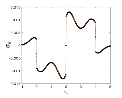
Figure 1: (Color online) $\sigma_{n}$ (in units of $\frac{e^{2}}{h}$), which quantifies the response of the system to the quantized part of field, as a function of $e_{s}$ in a model with ${d_{x}}=\sin{k_{y}},{d_{y}}=\sin{k_{x}},{d_{z}}=2-\cos{k_{x}}-\cos{k_{y}}-e_{s}$. The other parameters chosen are $\delta_{E}=0.3$ meV/nm, $\bar{E}$=0.1meV/nm.

Physically, this model can be interpreted as a tight-binding model describing a magnetic semiconductor with Rashba type spin-orbit coupling, spin dependent effective mass and a uniform magnetization on $z-$direction. It has been shownqi06 that $\sigma_{c}=1$ for $0<e_{s}<2$; $\sigma_{c}=-1$ for $2<e_{s}<4$, and $\sigma_{c}=0$ for $e_{s}<0$ and $e_{s}>4.$

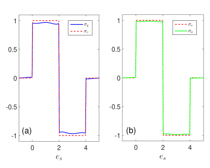
Figure 2: (color online) (a) Hall conductance $\sigma_{q}$(in units of $e^{2}/h$) as a function of $e_{s}.$ $\delta_{E}=0.3$ meV/nm, $n=4$. For comparison, the conventional Hall conductance (red-dashed line) is also shown. (b) Averaged Hall conductance $\sigma_{a}$ as a function of $e_{s}$. $\sigma_{a}$ is defined as ${\sigma_{a}}=\frac{1}{N}\sum_{j=1}^{N}\sigma_{q}(\delta_{E}^{j}),$ where $\delta_{E}^{j}$ denotes the $j-$th random value of $\delta_{E}$ from $[-0.3,0.3].$ Here $N=50$. $\vec{d}(\vec{k})$ is the same as in Fig. 1.

With respect to the photon number $n$, the Hall conductance $\sigma_{n}$ defined in Eq. (9) is plotted as a function of $e_{s}$ in Fig. 1. We find that the phase transition points, i.e., $e_{s}=0,2,4$ remain unchanged. In contrast with the well known Hall conductance $\sigma_{c}$ shown in Fig. 2 (red dashed lines), $\sigma_{n}$ is not a constant in regions, $0<e_{s}<2$, $2<e_{s}<4$, $e_{s}<0$ and $e_{s}>4.$ This results from the weight $\frac{\partial\cos\alpha_{q}^{-}}{\partial n}$ in the integral of Eq. (10). Physically, the weight plays the role of distribution function, which is not a constant and depends on $k_{x}$, $k_{y}$ and $e_{s}$ in this model. Fig. 2 shows $\sigma_{c}$, $\sigma_{a}$ and $\sigma_{q}$ as a function of $e_{s}$, where $\sigma_{a}$ is defined as $\sigma_{a}=\frac{1}{N}\sum_{j=1}^{N}\sigma_{q}(\delta_{E}^{j})$. $\delta_{E}^{j}$ denotes the $j-$th value of $\delta_{E}$ randomly chosen from $[-0.3,0.3],$ that is, $\sigma_{a}$ is defined as an average over $\delta_{E}$ chosen randomly in interval $[-0.3,0.3].$ Two observations can be made. (1) Quantum fluctuations suppress the Hall conductance $\sigma_{c}$, but they do not change the phase transition points; (2) $\sigma_{a}$ is very close to $\sigma_{c}$, suggesting that the quantum fields (fluctuations of the classical field) have small effect on the Hall conductance on average.

The second example we will take to illustrate the conductances is a two-dimensional lattice in a magnetic field kohmoto89 . The tight-binding Hamiltonian for such a lattice takes, $H=-t_{a}\sum\limits_{\left\langle{i,j}\right\rangle}{{}_{x}}c_{j}^{\dagger}{c_{i}}{e^{i{\theta_{ij}}}}-t_{b}\sum\limits_{\left\langle{i,j}\right\rangle}{{}_{y}}c_{j}^{\dagger}{c_{i}}{e^{i{\theta_{ij}}}},$ where $c_{j}$ is the usual fermion operator on the lattice. The phase $\theta_{ij}=-\theta_{ji}$ represents the magnetic flux through the lattice. When $t_{b}=0$, the single band is doubly degenerate. The term with $t_{b}$ in the Hamiltonian gives the coupling between the two branches of the dispersion. Consider two branches which are coupled by $|l|-$th order perturbation, the gaps open and the size of the gap due to this coupling is the order of $t_{b}^{|l|}$. The effective Hamiltonian then take the form of Eq. (1) with ${d_{x}}=\delta\cos{k_{y}},{d_{y}}=\delta\sin{k_{y}},{d_{z}}=2{t_{a}}\cos({k_{x}}+2\pi mp/q)$, where $p,q$ are integers, $\delta$ is proportional to (is the order of) $t_{b}^{\left|l\right|}.$

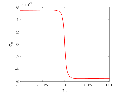
Figure 3: (Color online) $\sigma_{n}$ (in units of $\frac{e^{2}}{h}$) as a function of $t_{a}$. In this model, ${d_{x}}=\delta\cos{k_{y}},{d_{y}}=\delta\sin{k_{y}},{d_{z}}=2{t_{a}}\cos({k_{x}}+2\pi mp/q)$. The other parameters are $\delta_{E}=0.3$ meV/nm, $\bar{E}$=0.1meV/nm, $m=1,p=1,q=4$, $\delta=0.01$ meV.

From Fig. 3, we observe that $\sigma_{n}$ is very small, but it can witness the phase transition points. Fig. 4 shows the conventional Hall conductance $\sigma_{c}$, the Hall conductance $\sigma_{q}$ subject to the quantized field, and the averaged Hall conductance $\sigma_{a}$ as a function of $t_{a}.$ We find that the transition points remain unchanged, but the Hall conductance is slightly changed. The features observed from Fig. 3 and Fig. 4 support the conclusions made in Fig. 1 and Fig. 2. These observations suggests that the quantum Hall effect can be taken as a method to determine the fine structure constant even in the presence of quantum fluctuations.

It is worth noticing that all hall conductance including $\sigma_{q},$ $\sigma_{c}$ and $\sigma_{a}$ are zero when $\bar{E}=0,$ since in this case,

$$\bar{v}_{y}=\sin^{2}\frac{\alpha_{q0}}{2}\langle\varepsilon_{+}|v_{y}|\varepsilon_{+}\rangle+\cos^{2}\frac{\alpha_{q0}}{2}\langle\varepsilon_{-}|v_{y}|\varepsilon_{-}\rangle=0.$$

Here $\alpha_{q0}=\alpha_{q}^{-}(\bar{E}=0).$ In other words, a quantized field can not induce current in the system. This feature is reminiscent of the which-way experimentdurt98 ; buks98 that an attempt to gain information about the path taken by the particle inevitably reduces the visibility of the interference pattern. Here the quantum field can record the information of the path, while the classical field can not. Indeed, observing Eq.(7), we find that the current induced by the external field is very similar to the interference patten in the which-way experiment, where $|\varepsilon_{+}\rangle$ and $|\varepsilon_{-}\rangle$ play the role of the two paths.

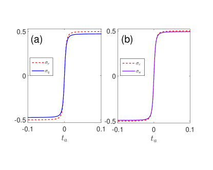
Figure 4: (color online) (a) Hall conductance $\sigma_{q}$ as a function of $t_{a}$. For comparison, the conventional Hall conductance $\sigma_{c}$ is also plotted. The model is ${d_{x}}=\delta\cos{k_{y}},{d_{y}}=\delta\sin{k_{y}},{d_{z}}=2{t_{a}}\cos({k_{x}}+2\pi mp/q)$. The other parameters chosen are $\delta_{E}=0.3$ meV/nm. (b) Averaged Hall conductance $\sigma_{a}$ versus $t_{a}$. $\sigma_{a}$ is defined in the same way as in Fig. 2. $\delta_{E}$ is randomly chosen from [-0.3,0.3] meV/nm for 50 times. The other parameters chosen for both (a) and (b) are $m=1,p=1,q=4,$ $\delta=0.01$ meV, $n=4.$ All conductances are plotted in units of $\frac{e^{2}}{h}$.

Consider the case without photon in the field and neglect the vacuum effect, i.e., $n=0$ and $\omega=0$, the change in Hall conductances (with respect to the conventional Hall conductance) can be understood as a consequence of band mixing caused by the quantum field, since the bulk band gaps remain open, see Fig. 5. In Fig. 5, we plot the energy spectrum of the system in the first example. $E_{d}$ denotes the spectrum of the system $H_{0}$ without external fields, $E_{c}$ stands for the spectrum of the system in the external field with $\delta_{E}=0$, and $E_{q}$ is the spectrum with $\delta_{E}\neq 0$. The interactions parameterized by $\bar{E}$ and $\delta_{E}$ enlarge the band gaps. So, the topological nature of the system remains unchanged.

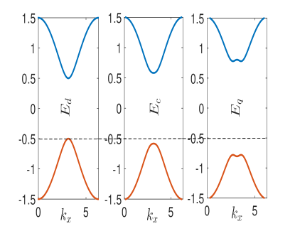
Figure 5: (Color online) Energy spectrum (in units of meV) of the system in the first example. The other parameters are $e_{s}=1.5$meV. $\delta_{E}=\bar{E}=0.3$ meV/nm, $n=0,\omega=0.$

The result changes when $n\neq 0$ and $\omega\neq 0.$ The quantized field (or the photon field) can change the topology of the system, see Fig.6. It is possible to switch between different topological phases by changing the photon number and the frequency, which may induces more avoid-crossing points as depicted in Fig.6. This observation is confirmed by an ac conductance $\sigma_{q}(\omega)$, which is defined in the same way as $\sigma_{q}$ but without the limitation of $\omega\rightarrow 0$ in Eq. (8).

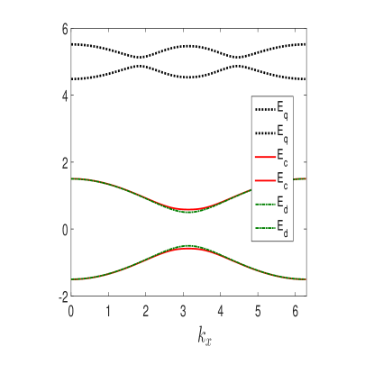
Figure 6: (Color online) The same as Fig. 5, but with $\omega=2,n=1.$

To show the ac conductance of the system in the first example, we calculate $\sigma_{q}(\omega)$ as a function of $e_{s}$ at various applied electric field frequencies $\omega$. The numerical results are shown in Fig. 7. The difference between $\sigma_{q}(\omega)$ with various $\omega$ arises because the photon field may induce more avoid-crossing points, which is depicted in Fig.6, lines for $E_{q}.$

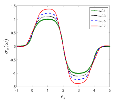
Figure 7: (Color online) Hall conductance $\sigma_{q}(\omega)$ ( in units of $\frac{e^{2}}{h}$) against $e_{s}$ at various frequencies of the external field. In this plot, ${d_{x}}=\sin{k_{y}},{d_{y}}=\sin{k_{x}},{d_{z}}=2-\cos{k_{x}}-\cos{k_{y}}-e_{s}$. The other parameters are $\delta_{E}=0.3$ meV/nm, $E_{x}=0.1$ meV/nm, $n=4.$

IV discussion and conclusion

The two-band model may describe topological insulators, which is realized by using either condensed matterlindner11 or cold atoms settingsjiang11 . The single mode field enters the system via a vector potential. The single photon mode is realized in a quantum LC circuithepp73 or is selected from a ladder of cavity models by placing a dispersive element into the caivty, of which the reflective index is wave-vector dependent. Tuning frequency $\omega$ and the coupling of the field with ITs is possible by changing the dielectric constant. The Hall conductance (equivalently the Chern number) can be probed through a Thouless typeye11 . The photon number may be tuned by a real-time quantum feedback procedure that generates on demand and stabilizes photon number states by reversing the effects of decoherence-induced quantum jumpssayrin11 . Alternatively, the photon number may be tuned via changing the coupling constant, since the square root of the photon number $\sqrt{n+1}$ always appears with the coupling constant $\eta.$

In summary, we have introduced the response of a two-band system to a quantized single-mode field. Three types of Hall conductance are introduced to quantify this response. Two examples are presented to exemplify the theory. Physics behind the findings is revealed and discussed.

Appendix A The result beyond the RWA

In this APPENDIX, we will present discussions on the results beyond the Rotating-wave approximation (RWA). We start with the Hamiltonian in the maintext,

$$H=\sum_{j=\pm}E_{j}^{c}|E_{j}^{c}\rangle\langle E_{j}^{c}|+\hbar\omega a^{\dagger}a+\eta(a^{\dagger}+a)|E_{+}^{c}\rangle\langle E_{-}^{c}|+h.c.$$ (12)

Notations are the same as in the maintext. To solve this Hamiltonian, we transform $H$ into an effective Hamiltonian,

$$H_{eff}=e^{s}He^{-s}=\sum_{j=\pm}E_{j}^{c}|E_{j}^{c}\rangle\langle E_{j}^{c}|+\hbar\omega a^{\dagger}a+g^{\prime}a|E_{+}^{c}\rangle\langle E_{-}^{c}|+h.c.$$ (13)

Here, $s=\frac{\Re({\eta})}{2E_{+}^{c}+\hbar\omega}\tau_{x}(a^{\dagger}-a)-\frac{\Im({\eta})}{2E_{+}^{c}+\hbar\omega}\tau_{y}(a^{\dagger}-a),$ and

$$g^{\prime}=\frac{4E_{+}^{c}}{2E_{+}^{c}+\hbar\omega}\eta,$$ (14)

The eigenstates of the effective Hamiltonian are then,

$$|E_{+}^{q}\rangle_{n}^{\prime}=\cos\frac{\alpha_{q}^{\prime}}{2}e^{i\beta_{q}^{\prime}}|E_{+}^{c}\rangle\otimes|n\rangle+\sin\frac{\alpha_{q}^{\prime}}{2}|E_{-}^{c}\rangle\otimes|n+1\rangle,$$

and

$$|E_{-}^{q}\rangle_{n}^{\prime}=\sin\frac{\alpha_{q}^{\prime}}{2}e^{i\beta_{q}^{\prime}}|E_{+}^{c}\rangle\otimes|n\rangle-\cos\frac{\alpha_{q}^{\prime}}{2}|E_{-}^{c}\rangle\otimes|n+1\rangle,$$

with $\alpha_{q}^{\prime}$ being defined by,

$$\cos\alpha_{q}^{\prime}=\frac{(2E_{+}^{c}-\hbar\omega)}{\sqrt{\Delta^{2}+4|g^{\prime}|^{2}(n+1)}},$$

and $\Delta=(2E_{+}^{c}-\hbar\omega).$ The corresponding eigenenergies are denoted by $E_{+}^{q\prime}(n)$ and $E_{-}^{q\prime}(n)$, respectively. Assuming band $|E_{-}^{q}\rangle_{n}^{\prime}$ is filled, we may calculate the current and the Hall conductance discussed above. Obviously, the Hall conductance takes the same formula except $\alpha_{q}^{\prime}.$ The difference between $\alpha_{q}^{\prime}$ and $\alpha_{q}$ originates from the coupling constant $g^{\prime}=\frac{4E_{+}^{c}}{2E_{+}^{c}+\hbar\omega}\eta.$ For points $\{\vec{k}\}$ satisfying (resonant condition) $2E_{+}^{c}=\hbar\omega,$ we have $g^{\prime}=\eta,$ i.e., no difference $g^{\prime}$ and $\eta$ at these resonant points. However, for the off-resonant points, $g^{\prime}$ and $\eta$ might be very different, which can lead to different topological phases.

References

(1) K. v. Klitzing, G. Dorda and M. Pepper, Phys. Rev. Lett. 45, 494 (1980).
(2) D. C. Tsui, H. L. Störmer and A. C. Gossard, Phys. Rev. Lett. 48, 1559 (1982).
(3) C. Nayak, S. H. Simon, A. Stern, M. Freedman and S. Das Sarma, Rev.
Mod. Phys. 80, 1083(2008); A. Y. Kitaev, Ann. Phys.
303, 2(2003); A. Stern and N. H. Lindner, Science
339, 1179(2013).
(4) M. Z. Hasan and C. L. Kane, Rev. Mod. Phys. 82, 3045 (2010), and references therein.
(5) X. L. Qi, and S. C. Zhang, Phys. Today, 63, 33(2010).
(6) D. J. Thouless, M. Kohmoto, M.P. Nightingale, and M. den Nijs, Phys. Rev. Lett. 49, 405(1982).
(7) F. D. M. Haldane, Phys. Rev. Lett. 61, 2015(1988).
(8) B. A. Bernevig, T. L. Hughes, and S. C. Zhang, Science
314, 1757(2006).
(9) M. König, S. Wiedmann, C. Brüne, A. Roth, H. Buhmann, L.
Molenkamp, X. L. Qi, and S.-C. Zhang, Science 318, 766
(2007).
(10) A. Roth, C. Brüne, H. Buhmann, L. W. Molenkamp, J. Maciejko,
X. L. Qi, and S. C. Zhang, Science 325, 294(2009).
(11) X. L. Qi and S. C. Zhang, Rev. Mod. Phys. 83, 1057 (2011).
(12) R. Kubo, J. Phys. Soc. Jpn. 12, 570 (1957).
(13) D. J. Thouless, Phys. Rev. B 27, 6083(1983).
(14) M. V. Berry and J. M. Robbins, Proc. R. Soc. Lond. A 442,659(1993).
(15) O. V. Kibis, Phys. Rev. B 81, 165433
(2010); O. V. Kibis, Phys. Rev. B 86, 155108 (2012).
(16) B. Dora, J. Cayssol, F. Simon, and R. Moessner,
Phys. Rev. Lett 108, 056602 (2012).
(17) M. Trif and Y. Tserkovnyak, Phys. Rev. Lett.
109, 257002 (2012).
(18) B. Gulasci and B. Dora, Phys. Rev. Lett.
115, 160401 (2015).
(19) S. Durt, T. Nonn, and G. Ramp, Nature 395,
33(1998).
(20) E. Buks, R. Schuster, M. Heiblum, D. Mahalu, V. Umansky, Nauture
391, 871(1998).
(21) X. L. Qi, Y. S. Wu, and S. C. Zhang, Phys. Rev. B 74, 085308(2006).
(22) M. Kohmoto, Phys. Rev. B 39, 11943 (1989).
(23) N. H. Lindner, G. Refael, and V. Galitski, Nat. Phys. 7, 490
(2011).
(24) L. Jiang, T. Kitagawa, J. Alicea, A. R. Akhmerov, D. Pekker, G.
Refael, J. I. Cirac, E. Demler, M. D. Lukin, and P. Zoller, Phys.
Rev. Lett. 106, 220402 (2011); N. Goldman, I. Satija, P.
Nikolic, A. Bermudez, M. A. Martin-Delgado, M. Lewenstein, and I. B.
Spielman, Phys. Rev. Lett. 105, 255302 (2010); F. Wilczek,
Phys. Rev. Lett. 109, 160401 (2012).
(25) K. Hepp and E. H. Lieb, Phys. Rev. A 8, 2517 (1973).
(26) J. Ye and C. Zhang, Phys. Rev. A 84, 023840 (2011).
(27)C. Sayrin, I. Dotsenko, X. Zhou, B.
Peaudecerf, T. Rybarczyk, S. Gleyzes, P. Rouchon, M. Mirrahimi, H.
Amini, M. Brune, J. Raimond, S. Haroche, Nature 477,
73(2011).