Gauge invariance of thermal transport coefficients

Abstract

Thermal transport coefficients are independent of the specific microscopic expression for the energy density and current from which they can be derived through the Green-Kubo formula. We discuss this independence in terms of a kind of gauge invariance resulting from energy conservation and extensivity, and demonstrate it numerically for a Lennard-Jones fluid, where different forms of the microscopic energy density lead to different time correlation functions for the heat flux, all of them, however, resulting in the same value for the thermal conductivity.

It has long been thought that the inherent indeterminacy of any quantum mechanical expression for the energy density would hinder the evaluation of thermal transport coefficients from equilibrium ab-initio molecular dynamics (AIMD), using the Green-Kubo (GK) formalism Green:1954 ; Kubo:1957 ; Kadanoff:1963 ; Forster . In classical molecular dynamics (CMD) this goal is achieved by decomposing the total energy of an extended system into localized atomic contributions and by deriving from this decomposition an explicit (and allegedly unique) expression for the energy flux. While the calculation of thermal transport coefficients from equilibrium AIMD has been successfully addressed by some of us in a recent work Marcolongo:2015 , the question still remains as to whether the expression for the energy flux currently used in CMD is uniquely defined and, in the negative, how is it that different definitions of the energy flux would lead to the same value for the thermal conductivity. In this paper we show that different equivalent definitions for the atomic energies in a classical system lead to different expressions for the macroscopic energy flux, and demonstrate numerically in the case of a Lennard-Jones fluid that these expressions result in the same value for the thermal conductivity, as evaluated from equilibrium CMD through the GK formula. This finding is then rationalized in terms of a kind of gauge invariance of heat transport coefficients, resulting from energy conservation and extensivity.

According to the GK formalism Green:1954 ; Kubo:1957 ; Kadanoff:1963 ; Forster , the heat conductivity $\kappa$ of an isotropic material can be expressed in terms of the auto-correlation function of the macroscopic heat flux, $\mathbf{J}_{q}(t)$, as:

$$\kappa=\frac{1}{3Vk_{B}T^{2}}\int_{0}^{\infty}\langle\mathbf{J}_{q}(t)\cdot\mathbf{J}_{q}(0)\rangle dt,$$ (1)

where brackets $\langle\cdot\rangle$ indicate canonical averages, $k_{B}$ is the Boltzmann constant, and $V$ and $T$ are the system volume and temperature, respectively. The heat flux is the macroscopic average of the heat current density, which is in turn defined as the non-convective component of the energy current density. Atoms in solids can be assumed to not diffuse, while in one-component and molecular fluids convective energy transport can be disregarded because of momentum conservation. Because of this, in the following we assume that energy and heat currents coincide.

In CMD the macroscopic energy flux is expressed in terms of suitably defined atomic energies whose sum yields the total energy of the system. For the sake of simplicity, we restrict our attention to one-component systems held together by pair potentials, in which case the atomic energies can be defined as Hansen:2006 :

$$\epsilon_{I}(\mathbf{R},\mathbf{V})=\frac{1}{2}MV_{I}^{2}+\frac{1}{2}\sum_{J\neq I}v(|\mathbf{R}_{I}-\mathbf{R}_{J}|),$$ (2)

where $M$ is the atomic mass, $\mathbf{R}\doteq\{\mathbf{R}_{I}\}$ and $\mathbf{V}\doteq\{\mathbf{V}_{I}\}$ are atomic coordinates and velocities, respectively, $v(R)$ is the inter-atomic pair potential, and the indices $I$ and $J$ run over all the atoms in the system. Using standard manipulations Hansen:2006 ; Lee:1991 , the macroscopic energy flux can be obtained from Eq. (2) as:

$$\mathbf{J}_{e}=\sum_{I}\epsilon_{I}\mathbf{V}_{I}-\frac{1}{2}\sum_{I,J\neq I}\bigl{(}\mathbf{V}_{I}\cdot\nabla_{I}v(|\mathbf{R}_{I}-\mathbf{R}_{J}|)\bigr{)}(\mathbf{R}_{I}-\mathbf{R}_{J}).$$ (3)

where (for a derivation of Eq. (3), valid for general many-body inter-atomic potentials Lee:1991 and its specialization to the present pair-potentials case, see the Appendix). It is often implicitly assumed that the well-definedness of thermal transport coefficients would stem from the uniqueness of the decomposition of the system’s total energy into localized, atomic, contributions. This assumption is manifestly incorrect, as any decomposition leading to the same value for the total energy as Eq. (2) should be considered as legitimate. The difficulty of partitioning a system’s energy into subsystems’ contributions is illustrated in Figure 1, which depicts a system made of two interacting subsystems. When defining the energy of each of the two susbsystems, an arbitrary decision has to be made as to how the interaction energy is partitioned. In the case depicted in Figure 1, for instance, the energy of each of the two subsystems can be defined as $\mathcal{E}(\Omega_{i})=E(\Omega_{i})+\frac{1}{2}(1\pm\gamma)W_{12}$, where $E(\Omega_{i})$ are the energies of the two isolated subsystems, $W_{12}$ their interaction energy, and $\gamma$ an arbitrary constant. In the thermodynamic limit, when the energy of any relevant subsystem is much larger than the interaction between any pairs of them, the value of the $\gamma$ constant is irrelevant. When it comes to definining energy densities (i.e. energies of infinitesimal portions of a system) or atomic energies, instead, the magnitude of the interaction between different susbsystems is comparable to the their energies, which become therefore intrinsically ill-defined.

$$E(\Omega_{1}\cup\Omega_{2}) =E(\Omega_{1})+E(\Omega_{2})+W_{12}\qquad$$

$$\overset{?}{=}\mathcal{E}(\Omega_{1})+\mathcal{E}(\Omega_{2})$$

Figure 1: The energy of an isolated system is the sum of the energies of its subsystems (as defined when they are isolated as well) plus the interaction among them, $W$, whose magnitude scales as the area of the interface, depicted in red. When defining the energies of individual subsystems, $\mathcal{E}$, $W$ has to be arbitrarily partitioned among them.

As a specific example, we consider the following definition for the atomic energies Marcolongo:2014 :

$$\epsilon_{I}^{\Gamma}(\mathbf{R},\mathbf{V})=\frac{1}{2}M_{I}\mathrm{V}_{I}^{2}+\frac{1}{2}\sum_{J\neq I}v(|\mathbf{R}_{I}-\mathbf{R}_{J}|)(1+\Gamma_{IJ}),$$ (4)

where $\Gamma_{IJ}=-\Gamma_{JI}$ is any antisymmetric matrix. As the inter-atomic potential appearing in Eq. (4) is symmetric with respect to the atomic indices, it is clear that the sum of all the atomic energies does not depend on $\Gamma$, thus making any choice of $\Gamma$ equally permissible. This trivial observation has deep consequences on the theory of thermal fluctuations and transport, because the value of the macroscopic energy flux, instead, depends explicitly on $\Gamma$, thus making one fear that the resulting transport coefficients would depend on $\Gamma$ as well. Using the same manipulations that lead from Eq. (2) to Eq. (3), for any choice of the $\Gamma$ matrix in Eq. (4), a corresponding expression for the macroscopic energy flux can be found, reading Marcolongo:2014 :

$$\mathbf{J}_{e}^{\Gamma}=\mathbf{J}_{e}+\frac{1}{2}\sum_{I,J\neq I}\Gamma_{IJ}\Bigl{(}v(|\mathbf{R}_{I}-\mathbf{R}_{J}|)\mathbf{V}_{I}+(\mathbf{V}_{I}\cdot\nabla_{I}v(|\mathbf{R}_{I}-\mathbf{R}_{J}|))(\mathbf{R}_{I}-\mathbf{R}_{J})\Bigr{)}.$$ (5)

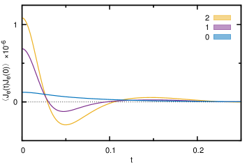
Figure 2: Time correlation functions of the modified macroscopic energy flux, as defined in Eq. (5), for different definitions of the $\Gamma$ matrix (see text). The “0” line refers to the original definition (i.e. $\Gamma=0$), whereas the label “1” and “2” correspond to the two definitions of the $\Gamma$ matrix given in Eq. (6). The parameters used are $\gamma_{1}=10$ and $\gamma_{2}=2.5$. Error bars, as estimated by standard block analysis, are smaller than the thickness of the lines. Units are Lennard-Jones units ($M=\sigma=\varepsilon=1$).

In order to illustrate this state of affairs, we have performed CMD simulations for a fluid of identical atoms, interacting through a Lennard-Jones potential: $v(R)=4\varepsilon\left[\left(\frac{\sigma}{R}\right)^{12}-\left(\frac{\sigma}{R}\right)^{6}\right]$ at density-temperature conditions $\rho=0.925\sigma^{-3}$ and $T=1.86\varepsilon/k_{B}$, using cubic simulation cells containing 256 atoms in the iso-choric microcanonical ensemble, $(NVE)$ LAMMPS:1995 . In Figure 2 we display the macroscopic energy-flux autocorrelation function corresponding to different choices of the $\Gamma$ matrix in Eqs. (4) and (5). The $\Gamma$ matrices have been constructed in two different ways, according to the prescriptions:

$$\Gamma_{IJ}=\left\{\begin{aligned} \frac{1}{2}\left(A_{IJ}-A_{JI}\right)&\quad\raise-492.47499pt\vbox{\small\noindent where the matrix elements of $A$ are drawn from a uniform deviate in the $[0,\gamma]$ interval.}&&\qquad(1)\\ \\ 0,+\gamma,-\gamma&\quad\raise-192.47499pt\vbox{\small\noindent according to whether $I=J$, $I>J$, or $I<J$.}&&\qquad(2)\\ \end{aligned}\right.$$ (6)

Figure 2 clearly shows that the $\langle\mathbf{J}_{e}^{\Gamma}(t)\cdot\mathbf{J}_{e}^{\Gamma}(0)\rangle$ correlation functions dramatically depend on the $\Gamma$ matrices in Eqs. (4) and (5). Notwithstanding, the integrals of all these time correlation functions tend to the same limit at large integration times, as displayed in Figure 3.

In order to get insight into this remarkable invariance property, let us inspect the difference between the generalized flux in Eq. (5) and the standard expression of Eq. (3):

$$\Delta\mathbf{J}_{e}^{\Gamma}=\mathbf{J}_{e}^{\Gamma}-\mathbf{J}_{e}=\frac{\mathrm{d}}{\mathrm{dt}}\frac{1}{4}\sum_{I,J\neq I}\Gamma_{IJ}\,v(|\mathbf{R}_{I}-\mathbf{R}_{J}|)(\mathbf{R}_{I}-\mathbf{R}_{J}).$$ (7)

We see that the two different expressions for the macroscopic energy flux differ by a total time derivative. In the following, we will show that this is a consequence of energy conservation and extensivity and a sufficient condition for the corresponding thermal conductivity to coincide.

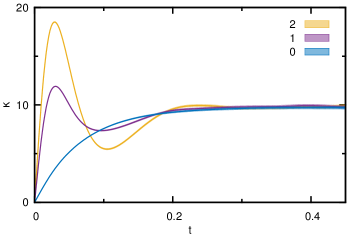
Figure 3: Integral of the time correlation functions displayed in Figure 2, multiplied by the prefactor appearing in the GK relation, Eq. (1), as a function of the upper limit of integration. Units are Lennard-Jones units (see caption to Figure 2). The barely visible shaded area surrounding each line is an indication of the error bars, as estimated by standard block analysis.

The very possibility of defining an energy current density stems from energy extensivity and conservation. Energy is extensive: because of this, the energy of a macroscopic sample of matter of volume $\Omega$ can be written as the integral of an energy density, $e(\mathbf{r})$:

$$E[\Omega]=\int_{\Omega}e(\mathbf{r})d\mathbf{r}.$$ (8)

Of course, the energy density appearing in Eq. (8) is not uniquely defined, the only requirement being that its integral over a domain $\Omega$ is well defined in the thermodynamic limit, i.e. two different densities whose integral over a domain $\Omega$ differ by a quantity that scales as the area of the domain boundary should be considered as equivalent. This equivalence can be expressed by the condition that two equivalent densities, say $e_{1}(\mathbf{r})$ and $e_{2}(\mathbf{r})$, differ by the divergence of a (bounded) vector field:

$$e_{2}(\mathbf{r})=e_{1}(\mathbf{r})+\nabla\cdot\mathbf{p}(\mathbf{r}).$$ (9)

In a sense, two equivalent energy densities can be thought of as different gauges of the same scalar field.

Energy is also conserved: because of this, for any given gauge of the energy density, $e(\mathbf{r})$, an energy current density can be defined, $\mathbf{j}_{e}(\mathbf{r},t)$, so as to satisfy the continuity equation:

$$\dot{e}(\mathbf{r},t)=-\nabla\cdot\mathbf{j}_{e}(\mathbf{r},t),$$ (10)

where the dot indicates a time derivative. By combining Eqs. (9) and (10) we see that energy current densities and macroscopic fluxes transform under a gauge transformation as:

$$\mathbf{j}_{2}(\mathbf{r},t) =\mathbf{j}_{1}(\mathbf{r},t)-\dot{\mathbf{p}}(\mathbf{r},t),$$ (11)

$$\mathbf{J}_{2}(t) =\mathbf{J}_{1}(t)-\dot{\mathbf{P}}(t),$$ (12)

where $\mathbf{P}(t)=\int\mathbf{p}(\mathbf{r},t)d\mathbf{r}$. We conclude that the macroscopic energy fluxes in two different energy gauges differ by the total time derivative of a vector.

Our previous findings on the energy flux of a system of classical atoms interacting through pair potentials as embodied in Eq. (7) can be recovered by defining the corresponding energy density as:

$$e(\mathbf{r})=\sum_{I}\delta(\mathbf{r}-\mathbf{R}_{I})\epsilon_{I}.$$ (13)

By taking the first moment of the continuity equation, Eq. (10), with respect to $\mathbf{r}$ and integrating by parts its right-hand side, one sees that the macroscopic average of the energy current density is the first moment of the time derivative of the energy density:

$$\mathbf{J}_{e}(t)=\int\dot{e}(\mathbf{r},t)\mathbf{r}~{}d\mathbf{r}.$$ (14)

Eq. (14) is ill-defined in periodic boundary conditions because the position variable appearing therein is defined modulo an integer translation, and the first moment of a periodic function depends therefore on the definition and choice of origin of the unit cell. This same difficulty affects the definition of the macroscopic polarization in insulators and has given birth to the so called modern theory of polarization Resta:2007 . Nevertheless, by throwing Eq. (13) into Eq. (14) and using Newton’s equations of motion, Eq. (14) can be cast into a boundary-insensitive form, as explained in detail in the Appendix, eventually resulting in the expressions for the macroscopic energy flux given by Eqs. (19) and (5).

We now show that the energy fluxes of the same system in two different energy gauges, $e_{1}$ and $e_{2}$, thus differing by a total time derivative, as in Eq. (12), result in the same heat conductivity, as given by the Green-Kubo formula, Eq. (1). Let us indicate by $\kappa_{1}$ and $\kappa_{2}$ the thermal conductivities in the two gauges. Using Eq. (12) and the property that classical time auto-correlation functions are even in time, one obtains:

$$\kappa_{2}=\kappa_{1}+\\ \frac{1}{6Vk_{B}T^{2}}\int_{-\infty}^{+\infty}\frac{d}{dt}\bigl{(}\langle\textbf{P}(-t)\cdot\mathbf{J}_{1}(0)\rangle-\langle\textbf{P}(t)\cdot\mathbf{J}_{1}(0)\rangle+\langle\textbf{P}(t)\cdot\dot{\mathbf{P}}(0)\rangle\bigr{)}dt.$$ (15)

The integral on the right-hand side of Eq. (15) vanishes because the correlation function of two observables at large time lags factorizes into the product of two time-independent average values and because the average value of the current $\mathbf{J}_{1}$, as well as of any total time derivative, vanishes at equilibrium. We conclude that the heat conductivities computed in different energy gauges coincide, as they must on physical grounds.

In this paper we have demonstrated that, while the heat flux is inherently undetermined at the atomic level, the heat conductivity resulting from it through the Green-Kubo formula is indeed well defined, as any measurable property must be. This indeterminacy stems from the liberty one has to formally unpack the total energy of an extended system into localized contributions in an infinite number of equivalent ways. We believe that this freedom can be exploited to design the definition of the local energy (be it in terms of atomic energies or energy densities), so as to optimise the convergence of computer simulations, regarding simulation length, system size, or both.

Appendix

In order to derive Eq. (19) from Eq. (14), let us first compute the time derivative of Eq. (13) using the definition of the atomic energies, Eq. (2), to obtain:

$$\dot{e}(\mathbf{r})=\sum_{I}\left[\epsilon_{I}\mathbf{V}_{I}\cdot\nabla\delta(\mathbf{R}_{I}-\mathbf{r})+\delta(\mathbf{r}-\mathbf{R}_{I})\sum_{J}\left(\frac{\partial\epsilon_{I}}{\partial\mathbf{V}_{J}}\cdot\dot{\mathbf{V}}_{J}+\frac{\partial\epsilon_{I}}{\partial\mathbf{R}_{J}}\cdot\mathbf{V}_{J}\right)\right],$$ (16)

where $\nabla\delta$ is the gradient of the $\delta$ function. We now insert Eq. (16) into Eq. (14), to obtain:

$$\mathbf{J}=\sum_{I}\epsilon_{I}\mathbf{V}_{I}+\sum_{I}\mathbf{R}_{I}\left(\mathbf{V}_{I}\cdot\mathbf{F}_{I}-\sum_{J}\mathbf{F}_{JI}\cdot\mathbf{V}_{J}\right),$$ (17)

where $\mathbf{F}_{I}=M_{I}\dot{\mathbf{V}}_{I}$ is the force acting on the $I$-th atom and $\mathbf{F}_{JI}=-\frac{\partial\epsilon_{I}}{\partial\mathbf{R}_{J}}$. Eq. (17) is not well defined in periodic boundary conditions because the position of the $I$-th atom, $\mathbf{R}_{I}$, is defined modulo a vector in the Bravais lattice and depends on the choice of the origin of the unit cell. In order to write a well defined expression for the current, we first note that $\mathbf{F}_{I}=\sum_{J}\mathbf{F}_{IJ}$. Inserting this relation into Eq. (17), one obtains:

$$\mathbf{J}=\sum_{I}\epsilon_{I}\mathbf{V}_{I}+\sum_{IJ}\mathbf{R}_{I}(\mathbf{V}_{I}\cdot\mathbf{F}_{IJ}-\mathbf{V}_{J}\cdot\mathbf{F}_{JI}).$$ (18)

Now in the second term of the second sum in Eq. (18) we can interchange the $IJ$ dummy indeces, to obtain:

$$\mathbf{J}=\sum_{I}\epsilon_{I}\mathbf{V}_{I}+\sum_{I,J\neq I}(\mathbf{V}_{I}\cdot\mathbf{F}_{IJ})(\mathbf{R}_{I}-\mathbf{R}_{J}).$$ (19)

Eq. (19) is well defined in periodic boundary conditions, because it depends on atomic positions only through differences between pairs of them. Note that this derivation does not depend on the assumption that atoms interact through pair potentials, and it holds in fact for general many-body inter-atomic potentials. When atoms interact through pair potentials, as it is the case considered in the present paper, and adopting the standard definition for the atomic energies, Eq. (2), one has: $\mathbf{F}_{IJ}=\frac{1}{2}\bigl{(}\delta_{IJ}\mathbf{F}_{I}-\nabla_{I}v(|\mathbf{R}_{I}-\mathbf{R}_{J}|)\bigr{)}$, where $\nabla_{I}$ indicates the gradient with respect to the position of the $I$-th atom. Throwing this expression into Eq. (19), one one finally obtains Eq. (3) used in the text. Similarly, one would obtain the modified energy flux of Eq. (5) from the definition for the atomic energies given in Eq. (4).

References

- (1) M. S. Green, J. Chem. Phys. 22, 398 (1954).
- (2) R. Kubo, J. Phys. Soc. Jpn. 12, 570 (1957).
- (3) L. P. Kadanoff and P. C. Martin, Ann. Phys. 24, 419 (1963).
- (4) D. Forster, Hydrodynamic fluctuations, broken symmetry, and correlation functions (Benjamin, Reading, 1975).
- (5) A. Marcolongo, P. Umari, and S. Baroni, Nature Physics, doi:10.1038/nphys3509 (2015).
- (6) J.-P. Hansen and I.R. McDonald, Theory of Simple Liquids (Third Edition, Elsevier, Philadelphia, 2006).
- (7) Y. Lee, R. Biswas, C. Soukoulis, C. Wang, C. Chan, and K.M. Ho, Phys. Rev. B, 43, 6573 (1991).
- (8) A. Marcolongo, SISSA PhD thesis, http://cm.sissa.it/thesis/2014/marcolongo.
- (9) CMD simulations have been performed using the LAMMPS code, see: S. Plimpton, J. Comp. Phys. 117, 1 (1995); http://lammps.sandia.gov.
- (10) R. Resta and D. Vanderbilt, Top. Appl. Phys. 105, 31 (2007).