Cohort Query Processing

Abstract

Modern Internet applications often produce a large volume of user activity records. Data analysts are interested in cohort analysis, or finding unusual user behavioral trends, in these large tables of activity records. In a traditional database system, cohort analysis queries are both painful to specify and expensive to evaluate. We propose to extend database systems to support cohort analysis. We do so by extending SQL with three new operators. We devise three different evaluation schemes for cohort query processing. Two of them adopt a non-intrusive approach. The third approach employs a columnar based evaluation scheme with optimizations specifically designed for cohort query processing. Our experimental results confirm the performance benefits of our proposed columnar database system, compared against the two non-intrusive approaches that implement cohort queries on top of regular relational databases.

1 Introduction

Table 1: Mobile Game Activity Table player time action role country gold $t_{1}$ 001 2013/05/19:1000 launch dwarf Australia 0 $t_{2}$ 001 2013/05/20:0800 shop dwarf Australia 50 $t_{3}$ 001 2013/05/20:1400 shop dwarf Australia 100 $t_{4}$ 001 2013/05/21:1400 shop assassin Australia 50 $t_{5}$ 001 2013/05/22:0900 fight assassin Australia 0 $t_{6}$ 002 2013/05/20:0900 launch wizard United States 0 $t_{7}$ 002 2013/05/21:1500 shop wizard United States 30 $t_{8}$ 002 2013/05/22:1700 shop wizard United States 40 $t_{9}$ 003 2013/05/20:1000 launch bandit China 0 $t_{10}$ 003 2013/05/21:1000 fight bandit China 0 Table 2: Results of $Q_{s}$ week avgSpent 2013-05-19 50 2013-05-26 45 2013-06-02 43 2013-06-09 42 2013-06-16 45

Internet applications often accumulate a huge amount of activity data representing information associated with user actions. Such activity data are often tabulated to provide insights into the behavior of users in order to increase sales and ensure user retention. To illustrate, Table 2 shows some samples of a real dataset containing user activities collected from a mobile game. Each tuple in this table represents a user action and its associated information. For example, tuple $t_{1}$ represents that player 001 launched the game on 2013/05/19 in Australia in a dwarf role.

An obvious solution to obtain insights from such activity data is to apply traditional SQL GROUP BY operators. For example, if we want to look at the players’ shopping trend in terms of the gold (the virtual currency) they spent, we may run the following SQL query $Q_{s}$.

SELECT week, Avg(gold) as avgSpent

FROM GameActions

WHERE action = "shop"

GROUP BY Week(time) as week

Executing this query against a sample dataset (of which Table 2 shows some records) results in Table 2, where each tuple represents the average gold that users spent each week. The results seem to suggest that there was a slight drop in shopping, and then a partial recovery. However, it is hard to draw meaningful insights.

There are two major sources that can affect human behavior [9]: 1) aging, i.e., people behave differently as they grow older and 2) social changes, i.e., people behave differently if the societies they live in are different. In our in-game shopping example, players tend to buy more weapons in their initial game sessions than they do in later game sessions - this is the effect of aging. On the other hand, social change may also affect the players’ shopping behavior, e.g., with new weapons being introduced in iterative game development, players may start to spend again in order to acquire these weapons. Cohort analysis, originally introduced in Social Science, is a data analytical technique for assessing the effects of aging on human behavior in a changing society [9]. In particular, it allows us to tease apart the effect of aging from the effect of social change, and hence can offer more valuable insights.

With cohort analytics, social scientists study the human behavioral trend in three steps: 1) group users into cohorts; 2) determine the age of user activities and 3) compute aggregations for each (cohort, age) bucket. The first step employs the so called cohort operation to capture the effect of social differences. Social scientists choose a particular action $e$ (called the birth action) and divide users into different groups (called cohorts) based on the first time (called birth time) that users performed $e$. Each cohort is then represented by the time bin (e.g., day, week or month) associated with the birth time . Each activity tuple of a user is then assigned to the same cohort that this user belongs to. In the second step, social scientists capture the effect of aging by partitioning activity tuples in each cohort into smaller sub-partitions based on age. The age of an activity tuple $t$ is the duration between the birth time of that user and the time that user performed $t$. Finally, aggregated behavioral measure is reported for each (cohort, age) bucket.

Back to our in-game shopping example, suppose we choose launch as the birth action and week as the cohort time bin interval, the activity tuples of player 001 are assigned to 2013-05-19 launch cohort since the activity tuple $t_{1}$ (called birth activity tuple) indicates that player 001 first launched the game at that week. We further partition activity tuples in 2013-05-19 launch cohort into sub-partitions identified by age. As an example, the activity tuple $t_{2}$ is partitioned into the week 1 age sub-partition. Finally, we report the average gold spent for each (cohort, age) bucket shown in Table 3 and visualized in Figure 1. Each row in Figure 1 represents the shopping trend of a cohort measured at different ages. For example, column $k$ (under the age section) reports the average expenditures of the cohorts at the $k$th week (i.e., age = $k$).

Table 3: Cohort Report for Shopping Trend

cohort	age (weeks)
	1	2	3	4	5
2013-05-19 (145)	52	31	18	12	5
2013-05-26 (130)	58	43	31	21
2013-06-02 (135)	68	58	50
2013-06-09 (140)	80	73
2013-06-16 (126)	86

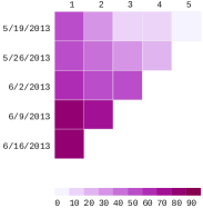
Figure 1: Launch Cohort Shopping Trend

By looking at each row horizontally, we can see the aging effect, i.e., players spent more gold on buying weapons on their initial game sessions than their later game sessions. For example, for the 2013-05-19 cohort, the amount of gold spent was 52 in the first week, but there is a clear declining trend as time passes. On the other hand, by comparing different rows (i.e., reading rows vertically), we can observe that the drop-off trend seems to becomes less severe. Comparing rows 1 and 2 in our example, we observe that for the same column, the value of row 2 is larger than that of row 1. This suggests that the iterative game development indeed did a better job of retaining player enthusiasm as they aged, an insight which cannot be drawn from OLAP style results in Table 2.

While the classic cohort analysis we presented so far has been very useful in many analytic applications such as retention analysis [1], we hope to 1) generalize the approach so that it can be applied to a wider range of applications and 2) extend SQL to support this generalized cohort analysis in this paper.

There are two limitations in the standard social science style cohort analysis. First, social scientists typically analyze a whole dataset. This is because the datasets used are usually small and are specifically collected for a certain cohort analysis task. As such, there is no mechanism for extracting a portion of users or activity tuples for cohort analysis. While this task seems trivial, it has to be handled with care as a naive selection may lead to incorrect answers! Referring to our running example (from Table 2), suppose we choose launch as the birth action, and we are interested to perform a cohort analysis on those tuples where time > 2013/05/22:0000. Now, the resultant subset of tuples is $\{t_{5},t_{8}\}$. However, we no longer can perform any cohort analysis as the birth activity tuple $t_{1}$, i.e., the activity tuple representing player 001 first performing launch, has been removed. Second, social scientists use only the time attribute to identify cohorts. This is because time is considered to be the key attribute that determines social change. However, it is possible that some other attributes, such as country, may also have a significant effect on social differences, in which case, it may be interesting to perform cohorts based on the country attribute. Thus, it would be desirable to provide support for a more general cohort analysis task.

WITH birth AS(

SELECT p, Min(t) as birthTime

FROM $D$

WHERE a = "launch"

GROUP BY p

),

birthTuples AS (

SELECT p, c as cohort, birthTime

role as birthRole

FROM $D$, birth

WHERE $D$.p = birth.p AND

$D$.t = birth.birthTime),

cohortT AS (

SELECT p, a, cohort, birthRole, gold

TimeDiff($D$.t, birthTime) as age

FROM $D$, birthTuples

WHERE $D$.p = birthTuples.p),

cohortSize AS (

SELECT cohort, Count(distinct p) as size

FROM cohortT

GROUP BY cohort

),

SELECT cohort, size, age, Sum(gold)

FROM cohortT, cohortSize

WHERE cohortT.cohort = cohortSize.cohort

birthRole = "dwarf" AND a = "shop" AND age > 0

GROUP BY cohort, age

Figure 2: The SQL query $Q_{s}$ of our example analysis task.

In this paper, we make the following contributions to address the above issues.

• We define the important problem of cohort analytics in the context of a DBMS.

• We introduce an extended relation to model user activity data for cohort analytics, and introduce three new operators for manipulating the extended relation and composing cohort queries. Two of the operators are designed for extracting a subset of activities for cohort analysis, and the last one is designed for producing aggregates over arbitrary attribute combinations. We show that cohort queries can be expressed elegantly and concisely using the data model and the newly proposed operators. We also show how more complicated data analytics tasks can be expressed using a mix of traditional SQL clauses and the newly proposed operators.

• We build a columnar based cohort query engine, COHAHA, which implements multiple optimizations for efficient cohort query processing.

• We design a benchmark study to compare COHANA against alternative non-intrusive evaluation schemes in terms of cohort query processing performance. The experimental results show that COHANA is two orders superior to its mostly optimized counterpart, demonstrating the necessity of extending database systems to cater to cohort analytics, rather than simply running an SQL statement over a traditional DBMS.

The rest of the paper is organized as follows: Section 2 presents the SQL based and the materialized view based approaches for processing cohort queries. Section 3 presents the foundations of cohort analysis. Section 4 presents our proposed columnar database based scheme for cohort query processing. Section 5 reports the experimental results. We present related work in Section 6 and conclude in Section 7.

2 Non-intrusive Approaches to Cohort Analytics

A least intrusive approach to supporting cohort analytics is to use an existing relational DBMS and express the cohort analysis task as a SQL query. We illustrate such an approach using the following cohort analysis task:

Example 1.

Given the launch birth action and the activity table as shown in Table 2 (denoted as $D$), for players who play the dwarf role at their birth time, cohort those players based on their birth countries and report the total gold that country launch cohorts spent since they were born.

Figure 2 shows the corresponding SQL query $Q_{s}$ for this task. To save space, we use p, a, t, c abbreviations respectively to denote the player, action, time, and country attribute in Table 2. The $Q_{s}$ employs four sub-queries (i.e., Figure 2 – Figure 2) and one outer query (i.e., Figure 2) to produce the results. Overall, this SQL approach performs poorly for three reasons:

• The SQL statement $Q_{s}$ is verbose, and its complexity renders it prone to mistakes.

• The SQL statement $Q_{s}$ requires many joins to perform the analysis task. As we shall see in our experimental study, such a query processing scheme can be up to 5 orders of magnitude slower than our proposed solution.

• It requires manual tuning. For example, one may notice that we can push the selection condition (i.e., birthRole = "dwarf") from the outer query (Figure 2) to the inner sub-query (Figure 2) to reduce the size of intermediate tables. Ideally, such an optimization can be performed by an intelligent optimizer. However, our evaluation shows that few database systems can perform such an optimization.

To speed up the processing of the analysis task, we can adopt a materialized view (MV) approach that stores some intermediate results. For example, we can materialize the intermediate table cohortT produced by the sub-query in $Q_{s}$ (Figure 2) as follows.

CREATE VIEW MATERIALIZED cohorts as cohortT

With cohorts, we can express the query $Q_{S}$ in a simpler SQL statement consisting of a single sub-query (Figure 2) and an outer query (Figure 2). The performance of the resulting SQL expression is also improved since it only involves a single join. However, the materialized view approach also suffers from a number of issues.

• The cost of generating the MV is still high since it involves two joins (Figure 2 and 2).

• The storage space for the MV is huge if the approach is used as a general cohort query processing strategy. Figure 2 only includes a single calculated birth attribute birthRole as it is the only attribute appearing in the birth selection condition (i.e., the condition of playing as the dwarf role at birth time) of the analysis task. However, if other calculated birth attributes are also involved in the birth selection condition, we need to include those attributes in the MV as well. In the extreme case, every possible birth attribute shall be included in the MV, doubling the storage space as compared to the original activity table.

• The MV only answers cohort queries introduced by launch birth action. If another birth action (e.g., shop) is used, one more MV is required. Obviously, this per birth action per MV approach does not scale even for a small number of birth actions due to the cost of MV construction and maintenance.

• The query performance is still not optimal. By the definition of the analysis task, if a player does not play as dwarf role when that player is born, we should exclude all activity tuples of that player in the result set. Ideally, this filtering operation can be performed by simply checking the single birth activity tuple of that player. If the birth activity tuple indicates that the player is not qualified, we can safely skip all activity tuples of that player without further checking. However, as shown in Figure 2, the MV approach needs to, unnecessarily, check each activity tuple of a player to perform the filtering operation (i.e., comparing the value in birthRole attribute against dwarf). Building an index on the birthRole attribute cannot improve the situation much since index look up will introduce too many random seeks on large activity tables.

3 Cohort Analysis Foundations

In this paper, we seek to extend an existing relational database system to support cohort analytics. This section presents the data model, which includes a central new concept of an activity table, and the proposed new cohort operators.

We use the term cohort to refer to a number of individuals who have some common characteristic in performing a particular action for the first time; we use this particular action and the attribute values of the common characteristics to identify the resulting cohort. For example, a group of users who first login (the particular action) in 2015 January (the common characteristic) is called the 2015 January login cohort. Similarly customers who make their first purchase in the United States form a United States purchase cohort. Broadly speaking, cohort analysis is a data exploration technique that examines longitudinal behavioral trends of different cohorts since they were born.

3.1 Data Model

We represent a collection of activity data as an instance of an activity relation, a special relation where each tuple represents the information associated with a single user activity. We will also call an activity relation an activity table. In this paper, the two terms, i.e., activity relation and activity table are used interchangeably.

Formally, an activity table $D$ is a relation with attributes $A_{u},A_{t},A_{e},A_{1},\ldots,A_{n}$ where $n\geq 1$. $A_{u}$ is a string uniquely identifying a user; $A_{e}$ is also a string, representing an action chosen from a pre-defined collection of actions, and $A_{t}$ records the time at which $A_{u}$ performed $A_{e}$. Every other attribute in $D$ is a standard relational attribute. Furthermore, an activity table has a primary key constraint on $(A_{u},A_{t},A_{e})$. That is, each user $i$ can only perform a specific action $e$ once at each time instant. As exemplified in Table 2, the first three columns correspond to the user ($A_{u}$), timestamp ($A_{t}$) and action ($A_{e}$) attribute, respectively. Role and Country are dimension attributes, which respectively specify the role and the country of player $A_{u}$ when performing $A_{e}$ at $A_{t}$. Following the two dimension attributes is gold, a measure attribute representing the virtual currency that player $A_{u}$ spent for this action. We shall continue to use Table 2 as our running example for describing each concept in cohort analysis.

3.2 Basic Concepts of Cohort Analysis

We present three core concepts of cohort analysis: birth action, birth time and age. Given an action $e\in\operatorname{Dom}(A_{e})$, the birth time of user $i$ is the first time that $i$ performed $e$ or -1 if $i$ never performed $e$, as shown in Definition 1. An action $e$ is called a birth action if $e$ is used to define the birth time of users.

Definition 1.

Given an activity table $D$, and a birth action $e\in\operatorname{Dom}(A_{e})$, a time value $t^{i,e}$ is called the birth time of user $i$ if and only if

$$t^{i,e}=\left\{\begin{array}[]{ll}\min\pi_{A_{t}}(\sigma_{A_{u}=i\wedge A_{e}=e}(D))&if\quad\sigma_{A_{u}=i\wedge A_{e}=e}(D)\neq\emptyset\\ -1&otherwise\end{array}\right.$$

where $\pi$ and $\sigma$ are the standard projection and selection operators.

Definition 2.

Given an activity table $D$, and a birth action $e\in\operatorname{Dom}(A_{e})$, a tuple $d^{i,e}\in D$ is called the birth activity tuple of user $i$ if and only if

$$d^{i,e}[A_{u}]=i\wedge d^{i,e}[A_{t}]=t^{i,e}$$

Since $(A_{u},A_{t},A_{e})$ is the primary key of $D$, we conclude that for each user $i$, there is only one birth activity tuple of $i$ in $D$ for any birth action $e$ that $i$ performed.

Definition 3.

Given the birth time $t^{i,e}$, a numerical value $g$ is called the age of user $i$ in tuple $d\in D$, if and only if

$$d[A_{u}]=i\wedge t^{i,e}>=0\wedge g=d[A_{t}]-t^{i,e}$$

The concept of age is designed for specifying the time point to aggregate the behavioral metric of a cohort. In cohort analysis, we calculate the metric only at positive ages. That is, if the age of an user in a tuple is negative, that tuple will be excluded from the final report. The activity tuple with a positive age is called an age activity tuple. Furthermore, in practical applications, the age $g$ is normalized by a certain time unit such as a day, week or month. Without loss of generality, we assume that the granularity of $g$ is a day.

Consider the example activity relation in Table 2. Suppose we use the action launch as the birth action. Then, the activity tuple $t_{1}$ is the birth activity tuple of player 001, and the birth time is 2013/05/19:1000. The activity tuple $t_{2}$ is an age tuple of player 001 produced at age 1.

3.3 Cohort Operators

We now present operations on a single activity table. In particular, we propose two new operators to retrieve a subset of activity tuples for cohort analysis. We also propose a cohort aggregation operator for aggregating activity tuples for each (cohort, age) combination. As we shall see, these three operators enable us to express a cohort analysis task in a very concise and elegant way that is easy to understand.

3.3.1 The $\sigma^{b}_{C,e}$ Operator

The birth selection operator $\sigma^{b}_{C,e}$ is used to retrieve activity tuples of qualified users whose birth activity tuples satisfy a specific condition $C$.

Definition 4.

Given an activity table $D$, the birth selection operator $\sigma^{b}_{C,e}$ is defined as

$$\sigma^{b}_{C,e}(D)=\{d\in D\,|\,i\leftarrow d[A_{u}]\wedge C(d^{i,e})=\text{true}\}$$

where $C$ is a propositional formula and $e$ is a birth action.

Consider the activity relation $D$ in Table 2. Suppose we want to derive an activity table from $D$ which retains all activity tuples of users who were born from performing launch action in Australia. This can be achieved with the following expression, which returns $\{t_{1},t_{2},t_{3},t_{4},t_{5}\}$.

$$\sigma^{b}_{\text{country}=\text{Australia},\text{launch}}(D)$$

3.3.2 The $\sigma^{g}_{C,e}$ Operator

The age selection operator $\sigma^{g}_{C,e}$ is used to generate an activity table from $D$ which retains all birth activity tuples in $D$ but only a subset of age activity tuples which satisfy a condition $C$.

Definition 5.

Given an activity table $D$, the age selection operator $\sigma^{g}_{C,e}$ is defined as

$$\sigma^{g}_{C,e}(D)= \{d\in D|i\leftarrow d[A_{u}]\wedge$$

$$((d[A_{t}]=t^{i,e})\vee(d[A_{t}]>t^{i,e}\wedge C(d)=\text{true}))\}$$

where $C$ is a propositional formula and $e$ is a birth action.

For example, suppose shop is the birth action, and we want to derive an activity table which retains all birth activity tuples in Table 2 but only includes age activity tuples which indicate users performing in-game shopping in all countries but China. The following expression can be used to obtain the desired activity table.

$$\sigma^{g}_{\text{action}=\text{shop}\wedge\text{country}\neq\text{China},\text{shop}}(D)$$

The result set of the above selection operation is $\{t_{2},t_{3},t_{4},t_{7},t_{8}\}$ where $t_{2}$ is the birth activity tuple of player 001, $t_{3}$ and $t_{4}$ are the qualified age activity tuples of player 001. The activity tuples $t_{7}$ and $t_{8}$ are the birth activity tuple and the qualified age activity tuple of player 002.

A common requirement in specifying $\sigma^{g}_{C,e}$ operation is that we often want to reference the attribute values of birth activity tuples in $C$. For example, given the birth action shop, we may want to select age activity tuples whose users perform in-game shopping at the same location as their country of birth. We introduce a Birth() function for this purpose. Given an attribute $A$, for any activity tuple $d$, the Birth($A$) returns the value of attribute $A$ in $d[A_{u}]$’s birth activity tuple:

$$\textnormal{{Birth(}}\textnormal{\emph{$A$}}\textnormal{{)}}=d^{i,e}[A]$$

where $i=d[A_{u}]$ and $e$ is the birth action.

In our running example, suppose shop is the birth action, and we want to obtain an activity table which retains all birth activity tuples but only include age activity tuples which indicate that players performed shopping in the same role as they were born. The following expression is used to retrieve the desired results.

$$\sigma^{g}_{\text{role}=\texttt{Birth}(\text{role}),\text{shop}}(D)$$

The result set of the above operation is $\{t_{2},t_{3},t_{7},t_{8}\}$ where $t_{2}$ and $t_{7}$ are the birth activity tuples of player 001 and player 002, respectively, and $t_{3}$ and $t_{8}$ are the qualified age activity tuples.

3.3.3 The $\gamma^{c}_{\mathcal{L},e,f_{A}}$ Operator

We now present the cohort aggregation operator $\gamma^{c}_{\mathcal{L},e,f_{A}}$. This operator produces cohort aggregates in two steps: 1) cohort users and 2) aggregate activity tuples.

In the first step, given an activity table $D$ with its attribute set $\mathcal{A}$ and a birth action $e$, we pick up a cohort attribute set $\mathcal{L}\subset\mathcal{A}$ such that $\mathcal{L}\cap\{A_{u},A_{e}\}=\emptyset$ and assign each user $i$ to a cohort $c$ specified by $d^{i,e}[\mathcal{L}]$. Essentially, we divide users into cohorts based on the projection of users’ birth activity tuples onto a specified cohort attribute set.

In our running example, suppose launch is the birth action and the cohort attribute set is $\mathcal{L}$={country}, player 001 in Table 2 is assigned to the Australia launch cohort, player 002 is assigned to the United States launch cohort and player 003 is assigned to the China launch cohort.

After assigning users to cohorts, in the second step, we divide activity tuples (including both the birth activity tuples and the age activity tuples) into the same cohorts that the user belonged to for aggregation.

Definition 6.

Given an activity table $D$, the cohort aggregation operator $\gamma^{c}_{\mathcal{L},e,f_{A}}$ is defined as

$$\gamma^{c}_{\mathcal{L},e,f_{A}}(D)= \{(d_{\mathcal{L}},g,s,m)|$$

$$D_{g}\leftarrow\{(d,l,g)|d\in D\wedge i\leftarrow d[A_{u}]$$

$$\qquad\qquad\wedge l=d^{i,e}[\mathcal{L}]\wedge g=d[A_{t}]-t^{i,e}\}$$

$$\wedge(d_{\mathcal{L}},g)\in\pi_{l,g}(D_{g})$$

$$\wedge s=\text{Count}(\pi_{A_{u}}\sigma_{d_{g}[{l}]=d_{\mathcal{L}}}(D_{g}))$$

$$\wedge m=f_{A}(\sigma_{d_{g}[{l}]=d_{\mathcal{L}}\wedge d_{g}[g]=g\wedge g>0}(D_{g}))$$

where $\mathcal{L}$ is a cohort attributes set, $e$ is a birth action and $f_{A}$ is a standard aggregation function with respect to the attribute $A$.

In summary, the cohort aggregation operator takes an activity table $D$ as input and produces a normal relational table $R$ as output. Each row in the output table $R$ consists of four parts $(d_{\mathcal{L}},g,s,m)$, where $d_{\mathcal{L}}$ is the projection of birth activity tuples onto the cohort attributes set $\mathcal{L}$ and identifies the cohort, $g$ is the age, i.e., the time point that we report the aggregates, $s$ is the size of the cohort, i.e., the number of users in the cohort specified by $d_{\mathcal{L}}$, and $m$ is the aggregated measure produced by the aggregate function $f_{A}$. Note that we only apply $f_{A}$ on age activity tuples with $g>0$.

3.3.4 Properties of Cohort Operators

We note that the two selection operators, $\sigma^{b}_{C,e}$ and $\sigma^{g}_{C,e}$, are commutative if they involve the same birth action.

$$\sigma^{b}_{C,e}\sigma^{g}_{C,e}(D)=\sigma^{g}_{C,e}\sigma^{b}_{C,e}(D)$$ (1)

Based on this property, we can, as we shall see in Section 4, push the birth selection operator down the query plan to optimize cohort query evaluation.

3.4 The Cohort Query

Given an activity table $D$ and operators $\sigma^{b}_{C,e}$, $\sigma^{g}_{C,e}$, $\pi_{\mathcal{L}}$, and $\gamma^{c}_{\mathcal{L},e,f_{A}}$, a cohort query $Q:D\rightarrow R$ can be expressed as a composition of those operators that takes $D$ as input and produces a relation $R$ as output with the constraint that the same birth action $e$ is used for all cohort operators in $Q$. To specify a cohort query, we propose to use the following SQL-style SELECT statement.

SELECT ... FROM $D$

BIRTH FROM action = $e$ [ AND $\sigma^{b}_{C,e}$ ]

[ AGE ACTIVITIES IN $\sigma^{g}_{C,e}$ ]

COHORT BY $\mathcal{L}$

In the above syntax, $e$ is the birth action that is specified by the data analyst for the whole cohort query. The order of BIRTH FROM and AGE ACTIVITIES IN clauses is irrelevant, and the birth selection (i.e., $\sigma^{b}_{C,e}$) and age selection (i.e., $\sigma^{g}_{C,e}$) clauses are optional. We also introduce two keywords AGE and COHORTSIZE for data analysts to retrieve the calculated columns produced by $\gamma^{c}_{\mathcal{L},e,f_{A}}$ in the SELECT list. Note that except for projection, we disallow other relational operators such as $\sigma$ (i.e., SQL WHERE) and $\gamma$ (i.e., SQL GROUP BY), and binary operators like intersection and join, in a basic cohort query.

With the newly developed cohort operators, the cohort analysis task presented in Example 1 can be expressed by the following query:

$Q_{1}$: SELECT country, COHORTSIZE, AGE, Sum(gold) as spent

FROM $D$ AGE ACTIVITIES IN action = "shop"

BIRTH FROM action = "launch" AND role = "dwarf"

COHORT BY country

3.5 Extensions

Our cohort query proposal can be extended in many directions to enable even more complex and deep analysis. First, it would be great to mix cohort queries with SQL queries in a single query. For example, one may want to use a SQL query to retrieve specific cohort trends produced by a cohort query for further analysis. If the cohort operation is specified by multiple attributes (e.g., COHORT BY time, country, role), one may want to apply a SQL CUBE operator on top of the cohort query results for OLAP analysis. This mixed querying requirement can be achieved by applying the standard SQL WITH clause to encapsulate a cohort query as a sub-query that can be processed by an outer SQL query. The following example demonstrates how to use a mixed query to retrieve specific cohort spent trends reported by $Q_{1}$ for further analysis.

WITH cohorts AS ($Q_{1}$)

SELECT cohort, AGE, spent FROM cohorts

WHERE cohort IN ["Australia", "China"]

However, to ensure the correctness of a mixed query, certain rules must be established to prevent SQL queries from removing birth activity tuples incidently. First, for a mixed query, the outermost query must be a SQL query. That is, cohort queries can only serve as sub-queries inside a mixed query. Furthermore, we only allow SQL queries (no matter sub-queries or the outer query) to reference cohort sub-queries in the FROM or WHERE clauses and prohibit a cohort sub-query from referencing other SQL or cohort sub-queries. In addition, a mixed query should be evaluated in the order of first cohort sub-queries and then others. This “cohort query first” evaluation scheme ensures that no SQL queries can incidentally remove birth activity tuples during query processing.

Another extension is to introduce binary cohort operators (e.g., join, intersection etc.) for analyzing multiple activity tables. We leave the details of evaluating a mixed query and other interesting extensions in a future paper. In the rest of this paper, we shall focus on the approaches for evaluating a single cohort query over a single activity table.

3.6 Mapping Cohort Operations to SQL Statements

Before leaving this section, we shall demonstrate that given a materialized view (MV) built for a specific birth action, the proposed cohort operators can be implemented by SQL sub-queries. This enable us to pose cohort queries composed of newly developed operators in the context of a non-intrusive mechanism.

As shown in Section 2, the MV approach stores each activity tuple of user $i$ along with $i$’s birth attributes. Thus, to implement the birth selection operator, one can use a SQL SELECT statement with a WHERE clause specifying the birth selection condition on the materialized birth attributes. Similarly, the age selection operator can be simulated by a SQL SELECT statement with a WHERE clause specifying the age selection condition along with an additional predicate to include birth activity tuples. The cohort aggregation operator can be implemented by applying a SQL GROUP BY aggregation operation on the joined results between the cohortSize table and the qualified age activity tuples.

As an example, Figure 3 demonstrates for $Q1$ of Example 1 the correspondence between the three proposed cohort operators and the equivalent SQL statements posed on the MV built for the launch birth action. As in Figure 2, the player, action and time attributes are respectively abbreviated to p, a, and t. bc, br, bt and age are four attributes additionally materialized along with the original activity table. The first three attributes, bc, br and bt, respectively represent the birth attributes for country, role and time. It should be noted that the SQL statements of Figure 3 are separated out for ease of exposition: one can optimize them by combining Figure 3(a) and 3(b) into a single SQL statement, as we do in experiments.

WITH birthView AS(

SELECT p, a, t, gold,

bc, bt, age

FROM $MV$

WHERE br = "dwarf"

),

(a) $\sigma^{b}_{\text{role="dwarf", launch}}$

ageView AS (

SELECT *

FROM birthView

WHERE a = "shop" OR

(t=bt AND a="launch")

),

(b) $\sigma^{g}_{{\text{action="shop", launch}}}$

cohortSize AS (

SELECT bc as cohort,

Count(distinct p)

as size

FROM birthView

GROUP BY bc),

SELECT cohort, size, age,

Sum(gold) as spent

FROM ageView, cohortSize

WHERE cohort = bc

GROUP BY cohort, age

(c) $\gamma^{c}_{\text{country, launch, Sum(gold)}}$

Figure 3: The correspondence between cohort operators and SQL statements of the MV approach

4 COHANA: Cohort Query Engine

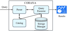
Figure 4: COHANA Architecture

To support cohort analytics with the newly designed cohort operators, we present four extensions to a columnar database: 1) a fine tuned columnar storage format for persisting activity tables; 2) a modified table scan operator capable of skipping age activity tuples of unqualified users; 3) a native efficient implementation of cohort operators; 4) a query planner capable of utilizing the cohort operator property (i.e., Equation (1)) for optimization. We have implemented the proposed techniques in a columnar based query engine, COHAHA, for performance study. Figure 4 presents the architecture of COHAHA which includes four modules: parser, catalog, storage manager and query executor. The first two modules are trivial, and we shall focus on the other two modules.

4.1 The Activity Table Storage Format

We store an activity table $D$ in the sorted order of its primary key $(A_{u},A_{t},A_{e})$. This storage layout has two nice properties: 1) activity tuples of the same user are clustered together; we refer to this as the clustering property; 2) The activity tuples of each user are stored in a chronological order; this is called the time ordering property. With these two properties, we can efficiently find the birth activity tuple of any user for any birth action in a single sequential scan. Suppose the activity tuples of user $i$ is stored between $d_{j}$ and $d_{k}$. To find the birth activity tuple of $i$ for any birth action $e$, we just iterate over each tuple between $d_{j}$ and $d_{k}$ and return the first tuple $d_{b}$ satisfying $d_{b}[A_{e}]=e$.

We employ a chunking scheme and various compression techniques to speed up cohort query processing. We first horizontally partition the activity table into multiple data chunks such that the activity tuples of each user are included in exactly one chunk. Then, in each chunk, the activity tuples are stored column by column. For each column in a data chunk, we choose an appropriate compression scheme for storing values based on the column type.

For the user column $A_{u}$, we choose Run-Length-Encoding (RLE) scheme. The values in $A_{u}$ is stored as a sequence of triples $(u,f,n)$, where $u$ is the user in $A_{u}$, $f$ is the position of the first appearance of $u$ in the column, and $n$ is the number of appearances of $u$ in the column. We shall see in Section 4.3, a modified table scan operator can directly process these triples and efficiently skip to the activity tuples of the next user if the birth activity tuple of the current user is not qualified with respect to the birth selection condition.

For the action column $A_{e}$ and other string columns, we employ a two level compression scheme presented in [11] for storing the values. More details of this encoding scheme can be found in [11]. For each such column $A$, we first build and persist a global dictionary which consists of the sorted unique values of $A$. Each unique value of $A$ is then assigned a global-id, which is the position of that value in the global dictionary. For each data chunk, the sorted global-ids of the unique values of $A$ in that chunk form a chunk dictionary. Given the chunk dictionary, each value of $A$ in that chunk can be represented as a chunk-id, which is the position of the global-id of that value in the chunk dictionary. The chunk-ids are then persisted immediately after the chunk dictionary in the same order as the respective values appear in $A$. This two level encoding scheme enables the efficient pruning of chunks where no users perform the birth action. For a given birth action $e$, we first perform a binary search on the global index to find its global-id $g_{i}$. Then, for each data chunk, we perform a binary search for $g_{i}$ in the chunk dictionary. If $g_{i}$ is not found, we can safely skip the current data chunk since no users in the data chunk perform $e$.

For $A_{t}$ and other integer columns, we employ a two-level delta encoding scheme which is similar to the one designed for string columns. For each column $A$ of this type, we first store the MIN and MAX value of $A$ for the whole activity table as the global range. Then, for each data chunk, the MIN and MAX values are extracted as the chunk range from the segment of $A$ in that chunk and persisted as well. Each value of the column segment is then finally stored as the delta (difference) between it and the chunk MIN value. Similar to the encoding scheme for string columns, this two-level delta encoding scheme also enables the efficient pruning of chunks where no activity tuples fall in the range specified in the birth selection or age selection operation.

With the above two encoding schemes, the final representation of string columns and integer columns are arrays of integers within a small range. We therefore further employ integer compression techniques to reduce the storage space. For each integer array, we compute the minimum number of bits, denoted by $n$, to represent the maximum value in the array, and then sequentially pack as many values as possible into a computer word such that each value only occupies $n$ bits. Finally, we persist the resulting computer words to the storage device. This fixed-width encoding scheme is by no means the most space-saving scheme. However, it enables the compressed values to be randomly read without decompression. For each position in the original integer array, one can easily locate the corresponding bits in the compressed computer words and extract the value from these bits. This feature is of vital importance for efficient cohort query processing.

4.2 Cohort Query Evaluation

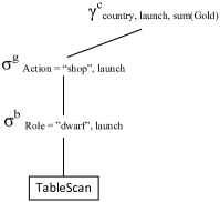
Figure 5: Query plan for $Q_{1}$

This section presents how to evaluate a cohort query over the activity table compressed with the techniques proposed in Section 4.1. We shall use the cohort query $Q_{1}$ as our running example. The overall query processing strategy is as follows. We first generate a logical query plan, and then optimize it by pushing down the birth selections along the plan. Next, the optimized query plan is executed against each data chunk. Finally, all partial results produced by the third step are merged together to produce the final result. The final merging step is trivial and we shall only present the first three steps.

The cohort query plan we introduced in this paper is a tree of physical operators consisting of four operators: TableScan, birth selection $\sigma^{b}_{C,e}$, age selection $\sigma^{g}_{C,e}$ and cohort aggregation $\gamma^{c}_{\mathcal{L},e,f_{A}}$. Like other columnar databases, the projection operation is implemented in a pre-processing step: we collect all required columns at query preparation stage and then pass those columns to the TableScan operator which retrieves the values for each column.

In the query plan, the root and the only leaf node are the aggregation operator, $\gamma^{c}_{\mathcal{L},e,f_{A}}$, and the TableScan operator, respectively, and between them is a sequence of birth selection operators and age selection operators.

Then, we push down the birth selection operators along the query plan such that they are always below the age selection operators. This push-down optimization is always feasible, since according to equation (1), we can arbitrarily swap the order of $\sigma^{b}_{C,e}$ and $\sigma^{g}_{C,e}$ operators in any sequence consisting of these two operators. Figure 5 shows the query plan for the cohort query of $Q_{1}$. We always employ this push-down optimization since, as we shall see in Section 4.3, a special designed TableScan implementation can efficiently skip age activity tuples without further processing for users whose birth activity tuples do not satisfy the birth selection condition. Therefore, the cost of evaluating birth selection operators before age selection operators is always less than the cost incurred from the reverse evaluation sequence in terms of the number of activity tuples processed.

After pushing down birth selections, the resulting query plan will be executed against each data chunk. Before the execution, we apply an additional filtering step by utilizing the $A_{e}$ column’s two-level compression scheme to skip data chunks where no users perform the birth action $e$. The concrete processing strategy is presented in Section 4.1. In practice, we find that this intermediate filtering step is particularly useful if the birth action is highly selective (i.e., only a few users performed that birth action).

We will present the implementation of the physical operators in the rest of this section.

4.3 The TableScan Operator

We augment the standard TableScan operator of columnar databases for efficient cohort query processing. The modified TableScan operator performs scanning operation over the compressed activity table that we proposed in Section 4.1. We mainly add two additional functions to a standard columnar database TableScan operator: GetNextUser() and SkipCurUser(). The GetNextUser() function returns the activity tuple block of the next user; the SkipCurUser() skips the activity tuples of the current user.

The modified TableScan operator is implemented as follows. For each data chunk, in the query initialization stage, the TableScan operator collects all (compressed) chunk columns referenced in the query and maintains for each chunk column a file pointer which is initialized to point to the beginning of that chunk column. The implementation of GetNext() function is identical to the standard TableScan operator of a columnar database.

The GetNextUser() is implemented by first retrieving the next triple $(u,f,n)$ of $A_{u}$ column and then advancing the file pointer of each other referenced column to the beginning of the column segment corresponding to user $u$. The SkipCurUser() is implemented in a similar way. When it is called, the SkipCurUser() function first calculates the number of remaining activity tuples of the current user, and then advances the file pointers of all columns by the same number.

4.4 Cohort Algorithms

This section develops algorithms for the implementation of cohort operators over the proposed storage format for activity tables.

Input : A data chunk $D$ and a birth action $e$

1

2GetBirthTuple($d,e$)

3       $i\leftarrow d[A_{u}]$

4       while $d[A_{u}]=i\wedge d[A_{e}]\neq e$ do

5             $d\leftarrow D$.GetNext()

6            

7      return $d$

8      

9

10Open()

11       $D$.Open()

12       $u_{c}\leftarrow\emptyset$

13      

14GetNext()

15       if $u_{c}$ has more activity tuples then

16             return $D.\textnormal{{GetNext(}}\textnormal{\emph{}}\textnormal{{)}}$

17      

18      while there are more users in the data chunk do

19             $(u,f,n)\leftarrow D.\textnormal{{GetNextUser(}}\textnormal{\emph{}}\textnormal{{)}}$

20             $u_{c}\leftarrow u$

21             $d\leftarrow D.\textnormal{{GetNext(}}\textnormal{\emph{}}\textnormal{{)}}$

22             $d^{b}\leftarrow\textnormal{{GetBirthTuple(}}\textnormal{\emph{$d,e$}}\textnormal{{)}}$

23             Found $\leftarrow C(d^{b})$

24             if Found then

25                   return $d$

26                  

27            $D.\textnormal{{SkipCurUser(}}\textnormal{\emph{}}\textnormal{{)}}$

28            

29      

Algorithm 1 $\sigma^{b}_{C,e}(D)$ operator implementation

Algorithm 1 presents the implementation of the birth selection operator $\sigma^{b}_{C,e}$. It employs an auxiliary function
GetBirthTuple($d,e$) (line 1 – line 5) for finding the birth activity tuple of user $i=d[A_{u}]$, given that $d$ is the first activity tuple of $i$ in the data chunk and $e$ is the birth action. The GetBirthTuple() function finds $i$’s birth activity tuple by iterating over each next tuple $d\in D$ and checks whether $d$ belongs to $i$ and whether $d[A_{e}]$ is the birth action $e$ (line 3). The first activity tuple $d$ matching the condition is the required birth activity tuple.

To evaluate $\sigma^{b}_{C,e}$, Algorithm 1 first opens the input data chunk $D$ and initializes the global variable $u_{c}$ (line 7 – line 8) which points to the user currently being processed. In the GetNext() function, we return the next activity tuple $d$ of $u_{c}$ if $u_{c}$ is qualified with respect to the birth selection condition (line 11). If $u_{c}$’s activity tuples are exhausted, we retrieve the next user block by calling the GetNextUser() function of the TableScan operator (line 13). Then, we find the birth activity tuple of the new user and check if it satisfies the birth selection condition (line 16 – line 17). If the new user is qualified, its birth activity tuple will be returned; otherwise all the activity tuples of this user will be skipped using the SkipCurUser() function so that its next user can be ready for processing. Therefore, one can continuously call the GetNext() function to retrieve the activity tuples of users that are qualified with respect to the birth selection condition.

The implementation of $\sigma^{g}_{C,e}$ is much simpler than $\sigma^{b}_{C,e}$. We also employ the user block processing strategy. For each user block, we first locate the birth activity tuple and then return the birth activity tuple and qualified age activity tuples.

Input : A data chunk $D$, a birth action $e$, an attribute list $\mathcal{L}$

1

2Open()

3       $D.\textnormal{{Open(}}\textnormal{\emph{}}\textnormal{{)}}$

4       $H^{c}\leftarrow\emptyset$ // Cohort size hash table

5       $H^{g}\leftarrow\emptyset$ // Cohort metric hash table

6       while there are more users in $D$ do

7             $(u,f,n)\leftarrow D.\textnormal{{GetNextUser(}}\textnormal{\emph{}}\textnormal{{)}}$

8             $u_{c}\leftarrow u$

9             $d\leftarrow D.\textnormal{{GetNext(}}\textnormal{\emph{}}\textnormal{{)}}$

10             $d^{b}\leftarrow D.\textnormal{{GetBirthTuple(}}\textnormal{\emph{$d,e$}}\textnormal{{)}}$

11             if $u_{c}$ is qualified then

12                   $H^{c}[d^{b}[\mathcal{L}]]++$

13                   while $u_{c}$ has more qualified age activity tuples do

14                         $g\leftarrow d[A_{t}]-d^{b}[A_{t}]$

15                         update $H^{g}[d^{b}[\mathcal{L}]][g]$ with $f_{A}(d)$

16                        

17                  

18            

19      

20

21GetNext()

22       Retrieve next key $(c,g)$ from $H^{g}$

23       return $(c,g,H^{c}[c],H^{g}[c][g])$

Algorithm 2 $\gamma_{\mathcal{L},e,f_{A}}(D)$ operator implementation

Algorithm 2 presents the implementation of $\gamma^{c}_{\mathcal{L},e,f_{A}}$ operator. The main logic is implemented in the Open() function. The function first initializes two hash tables $H^{c}$ and $H^{g}$ which respectively store the cohort size and per data chunk aggregation result for each (cohort, age) partition (line 2 – line 6). Then, the Open() function iterates over each user block and updates $H^{c}$ for each qualified user (determined by $\sigma^{b}_{C,e})$ and $H^{g}$ for all qualified age activity tuples (determined by $\sigma^{g}_{C,e}$) (line 10 – line 14). To speed up the query processing, we further follow the suggestions presented in [10, 11] and use array based hash tables for aggregation. In practice, we find that the use of array-based hash tables in the inner loop of cohort aggregation significantly improves the performance since modern CPUs can highly pipeline array operations.

4.5 Optimizing for User Retention Analysis

One popular application of cohort analysis is to show the trend of user retention [1]. These cohort queries involve counting distinct number of users for each (cohort, age) combination. This computation is very costly in terms of memory for fields with a large cardinality, such as $A_{u}$. Fortunately, our proposed storage format has a nice property that the activity tuples of any user are included in only one chunk. We therefore implement a UserCount() aggregation function for the efficient counting of distinct users by performing counting against each chunk and returning the sum of the obtained numbers as the final result.

4.6 Analysis of Query Performance

Given there are $n$ users in the activity table $D$, each user produces $m$ activity tuples, it can be clearly seen that, to evaluate a cohort query composed of $\sigma^{b}_{C,e}$, $\sigma^{g}_{C,e}$ and $\gamma^{c}_{\mathcal{L},e,f_{A}}$ operators, the query evaluation scheme we presented so far only needs to process $O(l\times m)$ activity tuples in a single pass, where $l$ is the number of qualified users with respect to the birth selection condition. Therefore, the query processing time grows linearly with $l$, and therefore approaches optimal performance.

5 A Performance Study

This section presents a performance study to evaluate the effectiveness of our proposed COHANA engine. We mainly perform two sets of experiments. First, we study the effectiveness of COHANA, and its optimization techniques. In the second set of experiments, we compare the performance of different query evaluation schemes. We implement the SQL based approach and the materialized view based approach on two relational databases: Postgres and MonetDB, and compare the performance of these two systems with COHANA. For the two relational databases, we allow them to use all the free memory for buffering, and leave all other settings as default.

5.1 Experimental Environment

All experiments are run on a high-end workstation. The workstation is equipped with a quad-core Intel Xeon E3-1220 v3 3.10GHz processor and 8GB of memory. The disk speed reported by hdparm is 14.8GB/s for cached reads and 138MB/s for buffered reads.

The dataset we used is produced by a real mobile game application. The dataset consists of 30M activity tuples contributed by 57,077 users worldwide from 2013-5-19 to 2013-06-26, and occupies a disk space of 3.6GB in its raw csv format. In addition to the required user, action and action time attributes, we also include the country, city and role as dimensions and session length and gold as measures. Users in the game played 16 actions in total, and we choose the launch, shop and achievement actions as the birth actions. In addition, we manually scale the dataset and study the performance of three cohort query evaluation schemes on different dataset size. Given a scale factor X, we produce a dataset consisting of X times users. Each user has the same activity tuples as the original dataset except with a different user attribute.

For the SQL based approach, we manually translate the cohort query into a SQL query as exemplified in Figure 2. For the materialized view approach, we manually materialize the view using CREATE TABLE AS command. For each birth action, we materialize the age and a birth attribute set of time, role, country and city attribute in its materialized view. This materialization scheme adds 15 additional columns to the original table by performing six joins in total. We also build a cluster index on the primary key and indices on birth attributes. For COHANA, we choose the chunk size to be 256K.

5.2 Benchmark Queries

We design four queries (described with COHANA’s cohort query syntax) for the benchmark by incrementally adding the cohort operators we proposed in this paper. The first query Q1 evaluates a single cohort aggregation operator. The second query Q2 evaluates a combination of birth selection and cohort aggregation. The third query Q3 evaluates a combination of age selection and cohort aggregation. The fourth query Q4 evaluates a combination of all three cohort operators. For each query, we report the average execution time of five runs for each system.

Q1: For each country launch cohort, report the number of retained users who did at least one action since they first launched the game.

SELECT country, CohortSize, Age, UserCount()

FROM GameActions BIRTH FROM action = "launch"

COHORT BY country

Q2: For each country launch cohort born in a specific date range, report the number of retained users who did at least one action since they first launched the game.

SELECT country, COHORTSIZE, AGE, UserCount()

FROM GameActions BIRTH FROM action = "launch" AND

time BETWEEN "2013-05-21" AND "2013-05-27"

COHORT BY country

Q3: For each country shop cohort, report the average gold they spent in shopping since they made first shop in the game.

SELECT country, COHORTSIZE, AGE, Avg(gold)

FROM GameActions BIRTH FROM action = "shop"

AGE ACTIVITIES IN action = "shop"

COHORT BY country

Q4: For each country shop cohort, report the average gold they spent in shopping in their birth country where they were born with respect to the dwarf role in a given date range.

SELECT country, COHORTSIZE, AGE, Avg(gold)

FROM GameActions BIRTH FROM action = "shop" AND

time BETWEEN "2013-05-21" AND "2013-05-27" AND

role = "dwarf" AND

country IN ["China", "Australia", "United States"]

AGE ACTIVITIES IN action = "shop" AND country = Birth(country)

COHORT BY country

In order to investigate the impact of the birth selection operator and the age selection operator on the query performance of COHANA, we further design two variants of Q1 and Q3 by adding to them a birth selection condition (resulting in Q5 and Q6) or an age selection condition (resulting in Q7 and Q8). The details of Q5-Q8 are shown below.

Q5: For each country launch cohort, report the number of retained users who did at least one action during the date range [d1; d2] since they first launched the game.

SELECT country, COHORTSIZE, AGE, UserCount()

FROM GameActions

BIRTH FROM action = "launch" AND time BETWEEN $d_{1}$ AND $d_{2}$

COHORT BY country

Q6: For each country shop cohort, report the average gold they spent in shopping during the date range [d1; d2] since they made their first shop in the game.

SELECT country, COHORTSIZE, AGE, Avg(gold)

FROM GameActions

BIRTH FROM action = "shop" AND time BETWEEN $d_{1}$ AND $d_{2}$

AGE ACTIVITIES IN action = "shop"

COHORT BY country

Q7: For each country launch cohort whose age is less than $g$, report the number of retained users who did at least one action since they first launched the game.

SELECT country, COHORTSIZE, AGE, UserCount()

FROM GameActions BIRTH FROM action = "launch"

AGE ACTIVITIES in AGE < $g$

COHORT BY country

Q8: For each country shop cohort whose age is less than $g$, report the average gold they spent in shopping since they made their first shop in the game.

SELECT country, COHORTSIZE, AGE, Avg(gold)

FROM GameActions BIRTH FROM action = "shop"

AGE ACTIVITIES IN action = "shop" AND AGE < $g$

COHORT BY country

5.3 Performance Study of COHANA

In this section we report on a set of experiments in which we vary chunk size and birth/age selection condition and investigate how COHANA adapts to such variation.

5.3.1 Effect of Chunk Size

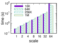
(a) Q1

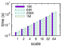
(b) Q2

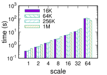
(c) Q3

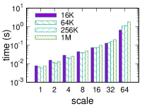
(d) Q4

Figure 6: COHANA’s performance under varying chunk size

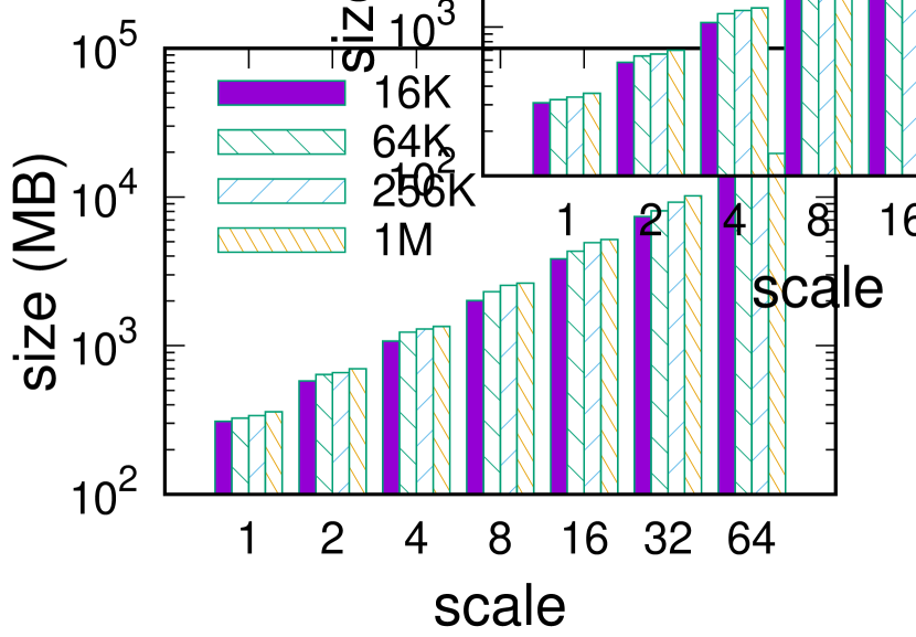
Figure 7: Effect of chunk size on storage space

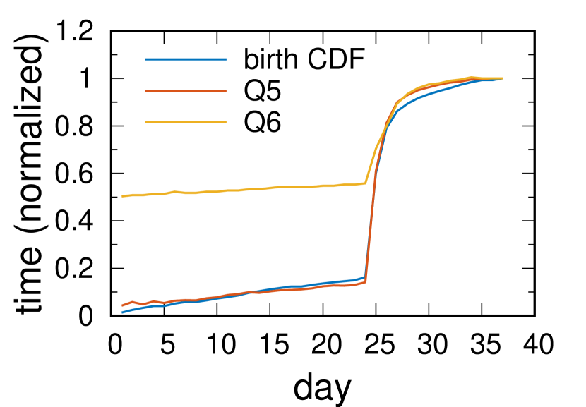
Figure 8: Effect of birth selection

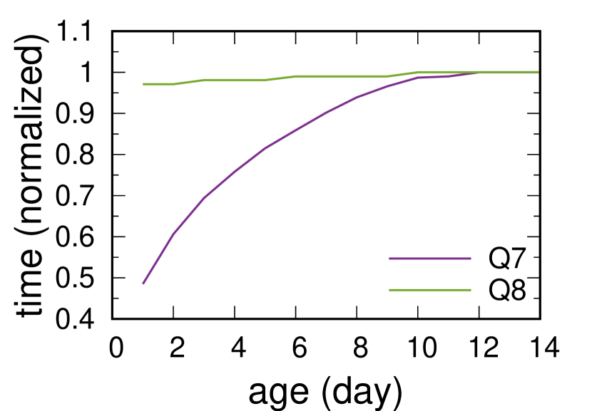
Figure 9: Effect of age selection  

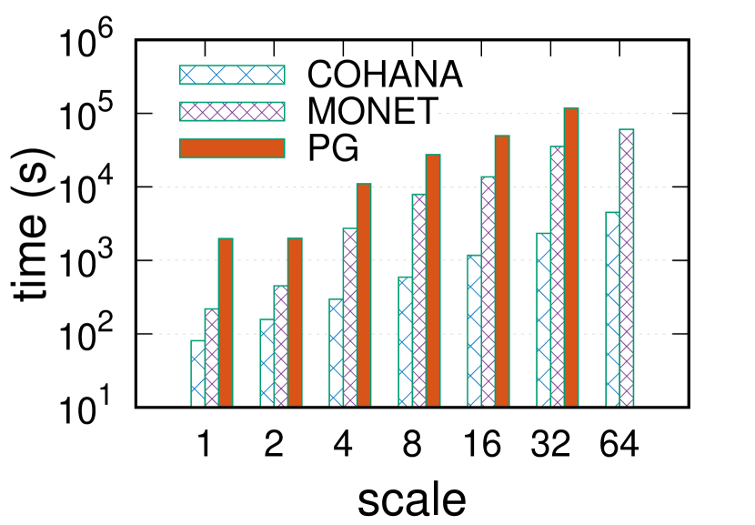
Figure 10: Time for generating MV

Figures 6 and 10 respectively present the storage space COHANA requires for the activity table compressed with different chunk sizes, and the corresponding query performance. It is clearly seen from Figure 10 that increasing the chunk size also augments storage cost. This is because an increase in the size of a chunk will lead to more players included in that chunk. As a result, the number of distinct values in the columns of each chunk also increases, which in turn requires more bits for encoding values. We also observe that cohort queries can be processed slightly faster under a smaller chunk size than a larger one. This is expected as fewer bytes are read. However, for large datasets, a larger chunk size can be a better choice. For example, at scale 64, COHANA processes Q1 and Q3 most efficiently under 1M chunk size. This is because the processing of Q1 and Q3 at scale 64 is dominated by disk accesses, whose granularity is normally a 4KB block. Compared with a large chunk size, a small one leads to more part of the neighbouring columns to be simultaneously read when reading a compressed chunk column, and hence results in a longer disk read time and a lower memory efficiency due to the memory contention between the useful columns and their unused neighbours within the same chunk.

5.3.2 Effect of Birth Selection

In Section 4.6, we claim that the running time of COHANA is bounded by $O(n)$ where $n$ is the total number of qualified users. This experiment studies the query performance of COHANA with respect to the birth selection selectivity. We run Q5 and Q6, which are respectively a variant of Q1 and Q3, by fixing $d1$ to be the earliest birth day, and incrementing $d2$ by one day each time. The dataset used in this experiment is at scale 1.

Figure 10 presents the processing times of Q5 and Q6 which are respectively normalized by that of Q1 and Q3. The cumulative distribution of user births is also given in this figure. We do not differentiate the birth distributions between the birth actions of launch and shop, as the birth distributions with respect to both birth actions are similar. It can be clearly observed from this figure that the processing time of Q5 highly coincides with the birth distribution. We attribute this coincidence to the optimization of pushing down the birth selection operator and the refined birth selection algorithm which is capable of skipping unqualified users. The processing time of Q6, however, is not very sensitive to the birth distribution. This is because in Q6, users are born with respect to the shop action, and there is a cost in finding the birth activity tuple for each user. This cost is avoided in Q5 as the first activity tuple of each user is the birth activity tuple of this user (recall that the first action each user performed is launch).

5.3.3 Effect of Age Selection

In this experiment, we run Q7 and Q8, another variant of Q1 and Q3, on the dataset of scale 1 by varying $g$ from 1 day to 14 days to study the query performance of COHANA under different age selection conditions. Figure 10 presents the result of this experiment. As in Figure 10, the processing times of Q7 and Q8 are also respectively normalized by that of Q1 and Q3. It can be seen from this figure that the processing times of Q7 and Q8 exhibit different trends. Specifically, the processing time of Q7 increases almost linearly, while the processing time for Q8 increases slowly. The reason for this difference is that the performance of Q7 is bounded by the number of distinct users within the given age range, which grows almost linearly with age range. For Q8, the processing time mainly depends on finding the birth activity tuples and the aggregation performed upon the shop activity tuples. The cost of the former operation is fixed across various age ranges, and the cost of the latter operation does not change dramatically as the number of shop activity tuples grows slowly with the age – the aging effect.

5.4 Comparative Study

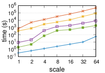
(a) Q1

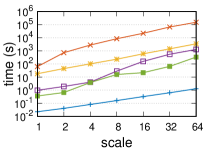
(b) Q2

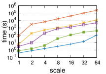
(c) Q3

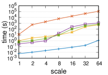
(d) Q4

Figure 11: Performance comparison among different evaluation schemes

Figure 11 reports for each scale (factor) the execution time that each system takes to execute the four queries. The results of the Postgres and the MonetDB databases are respectively shown in the lines labelled by “PG-S/M” and in those labelled by “MONET-S/M”, where “S” and “M” respectively mean the SQL and the materialized view approaches. As expected, the SQL based approach is the slowest as it needs multiple joins for processing cohort queries. With the elimination of joins, the materialized view based approach can reduce the query processing time by an order of magnitude. This figure also shows the power of columnar storage in terms of cohort query processing. MonetDB, a state-of-the-art columnar database, can be up to two orders faster than Postgres.

Although the combination of a materialized view and columnar storage can address cohort queries reasonably well on small datasets; however, it is not able to handle large datasets. For example, it takes half an hour to process Q1 at scale 64. The proposed system, COHANA, is able to perform extremely well not only on small datasets, but also on large datasets. Moreover, for each query, COHANA is able to perform better than the MonetDB equipped with the materialized view at any scale. The performance gap between them is one to two orders of magnitude in most cases, and can be up to three orders of magnitude (Q4 at scale 32). We also observe that the two retention queries (Q1 and Q2) enjoy a larger performance gain than Q3 does and in part attribute it to the optimization Section 4.5 presents for user retention analysis. Finally, the generation of the materialized view is much more expensive than COHANA. As shown in Figure 10, at scale 64, MonetDB needs more than 60,000 seconds (16.7 hours) to generate the materialized view from the original activity table. This time cost is even more expensive in Postgres, which needs more than 100,000 seconds (27.8 hours) at scale 32. The result for Postgres at scale 64 is not available as Postgres is not able to generate the materialized view before using up all free disk space, which also implies a high storage cost during the generation of the materialized view. In a sharp contrast, COHANA only needs 1.25 hours to compress the activity table of scale 64.

6 Related Work

The work related to ours is the database support for data analysis and cohort analysis. The requirement to support data analysis inside a database system has a long history. The early effort is the SQL GROUP BY operator and aggregate functions. These ideas are generalized with the CUBE operator [10]. Traditional row-oriented databases are inefficient for CUBE style OLAP analysis. Hence, columnar databases are proposed for solving the efficiency issue [7, 13, 15]. Techniques such as data compression [16, 18], query processing on compressed data [4, 6, 12], array based aggregation [5, 17], and materialized view based approaches [14] are proposed for speeding up OLAP queries. Albeit targeting OLAP queries which are defined on relational operators that are generally not applicable to cohort queries, the above techniques can also be used to accelerate the processing of cohort queries as we have shown in Section 4.

Cohort analysis originates from social science [9]. However, the cohort analysis approach presented in social science literatures has two limitations: 1) lack of a way for specifying a subset of users or activity tuples for analysis; 2) only use time attribute to identify cohorts. These two limitations are recognized in modern analytical software package [3, 1, 2]. These software somehow try to solve these limitations in their respective application domains. For example, MixPanel allows data analysts to select user segment for cohort analysis. But none of the solutions we investigated so far is general. For example, none of the software support Birth() filtering we present in this paper. An implicit cohort analysis is conducted in [8] to study the behavior of users in a private BitTorrent community using the SQL approach. Compared to the above works, our effort not only generalizes the cohort analysis for broader spectrum of applications, but also is the first attempt to extend database systems to support the generalized cohort analysis.

7 Conclusions

Cohort analysis is a powerful tool for finding unusual user behavioral trends in large activity tables. This paper has conducted the first investigation of database support for cohort analysis. Consequently, we have introduced an extended relation for modeling activity data and extended SQL with three new operators for composing cohort queries. We have developed a columnar based query engine, COHAHA, for efficient cohort query processing. Our experimental results showed that COHANA can achieve two orders faster query performance than simply running SQL queries over conventional database systems, demonstrating the possible benefit of extending a database system for cohort queries over implementing cohort queries on top of it.

References

- [1] Retention. https://mixpanel.com/retention/.
- [2] Rjmetrics. https://rjmetrics.com/.
- [3] Use the cohort analysis report. https://support.google.com/analytics/answer/6074676?hl=en.
- [4] D. Abadi, S. Madden, and M. Ferreira. Integrating compression and execution in column-oriented database systems. In SIGMOD, pages 671–682, 2006.
- [5] S. Agarwal, R. Agrawal, P. Deshpande, A. Gupta, J. F. Naughton, R. Ramakrishnan, and S. Sarawagi. On the computation of multidimensional aggregates. In VLDB, pages 506–521, 1996.
- [6] S. Amer-Yahia and T. Johnson. Optimizing queries on compressed bitmaps. In VLDB, pages 329–338, 2000.
- [7] P. A. Boncz, M. Zukowski, and N. Nes. Monetdb/x100: Hyper-pipelining query execution. In CIDR, pages 225–237, 2005.
- [8] Q. Cai and K.-T. Lo. A multi-faced measurement study on a large private bittorrent community. Peer-to-Peer Networking and Applications, 8(1):32–48, 2015.
- [9] N. D. Glenn. Cohort Analysis. Sage Publications, Inc., London, 2005.
- [10] J. Gray, A. Bosworth, A. Layman, and H. Pirahesh. Data cube: A relational aggregation operator generalizing group-by, cross-tab, and sub-total. In ICDE, pages 152–159, 1996.
- [11] A. Hall, O. Bachmann, R. Büssow, S. Ganceanu, and M. Nunkesser. Processing a trillion cells per mouse click. PVLDB, 5(11):1436–1446, 2012.
- [12] Y. Li and J. M. Patel. Bitweaving: Fast scans for main memory data processing. In SIGMOD, pages 289–300, 2013.
- [13] S. Manegold, P. A. Boncz, and M. L. Kersten. Optimizing database architecture for the new bottleneck: Memory access. The VLDB Journal, 9(3):231–246, 2000.
- [14] M. Staudt and M. Jarke. Incremental maintenance of externally materialized views. In VLDB, pages 75–86, 1996.
- [15] M. Stonebraker, D. J. Abadi, A. Batkin, X. Chen, M. Cherniack, M. Ferreira, E. Lau, A. Lin, S. Madden, E. O’Neil, P. O’Neil, A. Rasin, N. Tran, and S. Zdonik. C-store: A column-oriented dbms. In VLDB, pages 553–564, 2005.
- [16] T. Westmann, D. Kossmann, S. Helmer, and G. Moerkotte. The implementation and performance of compressed databases. SIGMOD Record, 29(3):55–67, 2000.
- [17] Y. Zhao, P. M. Deshpande, and J. F. Naughton. An array-based algorithm for simultaneous multidimensional aggregates. In SIGMOD, pages 159–170, 1997.
- [18] M. Zukowski, S. Heman, N. Nes, and P. Boncz. Super-scalar RAM-CPU cache compression. In ICDE, pages 59–70, 2006.