Time Dependent Study of Multiple Exciton Generation in Nanocrystal Quantum Dots

Abstract

We study the exciton dynamics in an optically excited nanocrystal quantum dot. Multiple exciton formation is more efficient in nanocrystal quantum dots compared to bulk semiconductors due to enhanced Coulomb interactions and the absence of conservation of momentum. The formation of multiple excitons is dependent on different excitation parameters and the dissipation. We study this process within a Lindblad quantum rate equation using the full many-particle states. We optically excite the system by creating a single high energy exciton $E_{SX}$ in resonance to a double exciton $E_{DX}$. With Coulomb electron-electron interaction, the population can be transferred from the single exciton to the double exciton state by impact ionisation (inverse Auger process). The ratio between the recombination processes and the absorbed photons provide the yield of the structure. We observe a quantum yield of comparable value to experiment assuming typical experimental conditions for a $4$ nm PbS quantum dot.

1 Introduction

Multiple exciton generation (MEG) is the process by which a single absorbed photon with high energy creates more than one electron hole pair  [1, 2, 3, 4]. It allows for converting the excess energy of absorbed photon into an additional photocurrent. In conventional solar cells based on bulk semiconductors, the conversion efficiency is limited and most of the excess energy is lost as heat within picosecond time scale after absorption. Due to quantum confinement effects, such as, relaxed momentum conservation, modified carrier-cooling rates, reduced dielectric screening of the quantum dot surface and enhanced Auger processes, an enhancement of MEG is expected in quantum dots compared to their bulk counterparts [5, 6]. Lead Chalcogenide QDs have been intensively studied in relation to MEG since the first demonstration of MEG in PbSe quantum dots  [4, 7]. These quantum dots are known to exhibit high confinement effects combined with a small band gap of bulk materials, e.g. $0.41$ eV for PbS and $0.28$ eV for PbSe at room temperature [8]. For a small lead based quantum dot, a quantum yield of $1.21\pm 0.05$ has been shown in a recent paper  [9] which means that the number of induced excitons surpassed the absorbed photons by about $20\%$. Apart from lead based dots, Cadmium Chalcogenide quantum dots, indium based quantum dots (InAs and InP) and Silicon quantum dots have been studied for exploring the efficiency of MEG in quantum dots  [10, 11, 12, 13, 14]. From an experimental perspective, very short time resolution and very low excitation fluence are two requirements that needs to be fulfilled when measuring MEG quantum yield [15]. The first requirement is due to the rapid Auger recombination ($\approx 10-100$ ps) [16] for multi-excitons in quantum dots in comparison to lifetime of single excitons ($\approx 10-100$ ns) [17]. To be able to capture these fast processes, techniques with time resolution much faster than the recombination times is needed. Ultrafast lasers can produce pulses as short as $100$ fs or less in duration which offer adequate time resolution needed [18]. The second requirement is to avoid multi-exciton formation due to successive excitation of quantum dots with two or more photons within the life time of a single exciton. The observation of multi-exciton recombination at low pump fluence can then be considered as the signature for MEG. Ultrafast transient absorption spectroscopy, which is a pump probe technique, is one of the mostly used experimental techniques for measuring MEG [19, 9, 20]. MEG in quantum dots has been simulated by several groups, with a strong focus on the impact ionisation process. Shabaev et al. [3] used a time dependent density matrix approach to study efficient MEG in nanocrystals as a coherent superposition of single and multi-exciton states and showed that efficient MEG is a consequence of suppressed thermalization rate of the initially excited single exciton. Allan et al. [21] showed that experimentally observed MEG yield in PbSe nanocrystals can be explained by impact ionisation process which is very efficient in PbSe and PbS nanocrystals with very fast ($\sim$ fs) lifetime for the single exciton to relax into the double exciton. Beard et al. [5] compared MEG in nanocrystal with impact ionisation in bulk and showed that the calculated quantum yield for nanocrystals is much larger than its bulk counterpart. The effect of relaxation has been studied by Schulze et al. [22]. In the same spirit, Azizi and Machnikowski [23] showed that relaxation can even increase the yield under certain conditions in a phenomenological three-state model.

In this work, we perform a quantum kinetic description based on a selected set of microscopic single particle states similar to [22]. However, we work in the corresponding many-body basis, which allows for a better identification of the exciton states. We use specific parameters for the recent experiment [9] with $4$ nm PbS dots, where MEG is studied after the excitation by a resonant pulse. This situation is schematically shown in Fig. 1(a). Within this method, the transient changes to the single exciton and double exciton states by the light pulse can be examined to see the various intermediate processes before the system relaxes to its ground state. Since the transient properties depend highly on the different parameters which can be controlled by suitable experimental setup, understanding these processes at the microscope level can greatly benefit for optimizing MEG experiments. The method can be used for similar quantum dot systems for interpreting experimental measurements on MEG yield and transient absorption experiments.

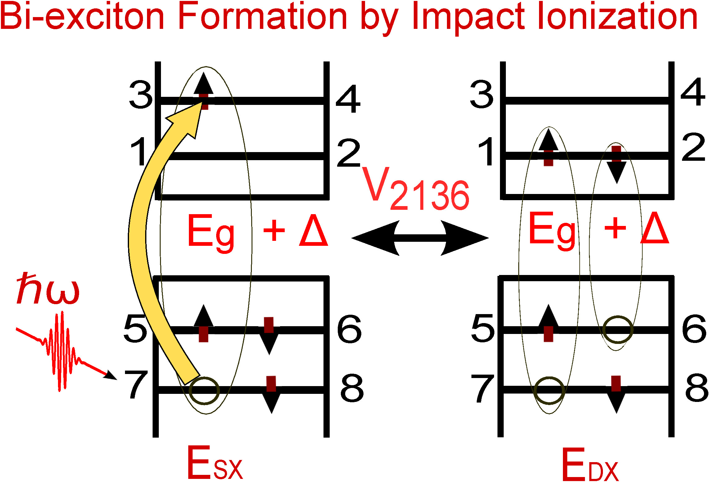
(a) Schematic single particle energies for the quantum dot considered showing the single exciton and double exciton configurations

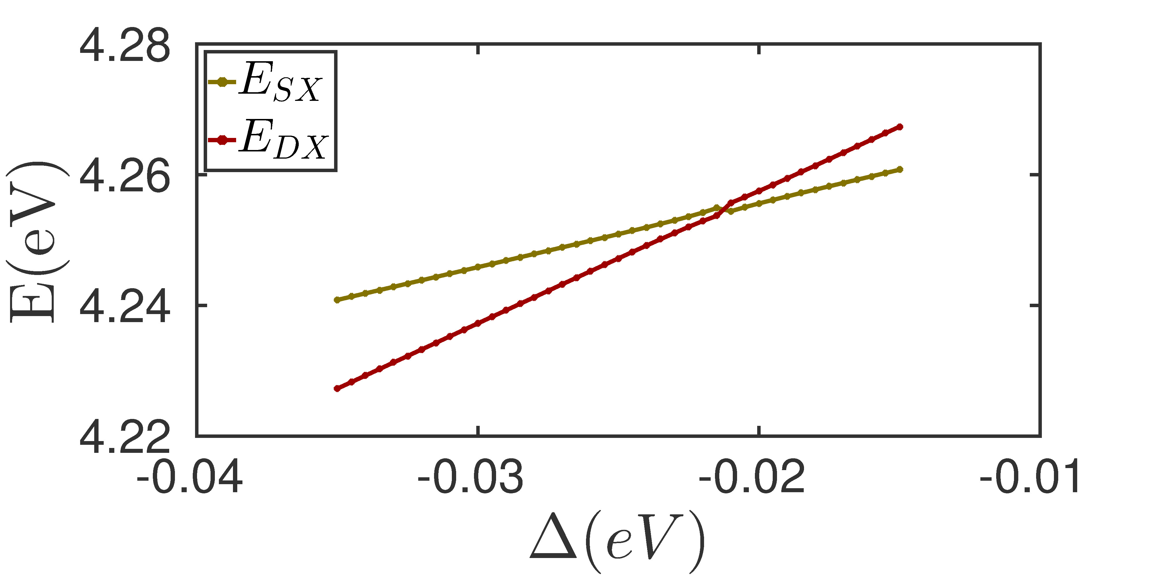
(b) Calculated energies of the high energy exciton $E_{SX}$ and double exciton $E_{DX}$ as a function of the parameter $\Delta$ taking into account all interactions.

Figure 1: Model studied and many particle energies of two important exciton states for the study

2 Method and Model

In order to describe the quantum kinetics in a PbS quantum dot under irradiation by a short laser pulse, we construct a set of many-body basis states which are diagonal with respect to the electron-electron interaction. Within this basis we formulate a Lindblad kinetics to include relaxation, recombination and dephasing. The different steps in the setup are addressed below.

2.1 Single particle levels

The energies of the single particle states for the spherical PbS quantum dot are evaluated using a K$\cdot$P method neglecting the multiplicity of valleys [8]. As an input for the K$\cdot$P calculations, the material parameters for PbS quantum dot were adopted from Table 1 of the paper  [8]. $m^{+}=m_{e}/3$ and $m^{-}=m_{e}/2.5$ are the conduction and valence band-edge effective masses respectively. The momentum-matrix element taken between the band-edge states of the conduction and valence band states is given by $P=\sqrt{2.5(eV)m_{e}/2}$. Here $m_{e}$ is the free electron mass. Furthermore, an energy gap $E_{g}=0.41$ eV at room temperature was also taken from the table. This gap is very narrow compared to most semiconductor materials which makes PbS quantum dots an excellent platform for studying MEG.

Orbital	n	l	$E^{c}_{nl}(eV)$	$E^{v}_{nl}(eV)$
1s	1	0	$E_{1/2}=0.650280$	$E_{5/6}=-0.6972889$
1p	1	1	0.964789	-1.0609576
1d	1	2	1.319638	-1.4778528
2s	2	0	1.482883	-1.6709188
1f	1	3	1.721845	-1.954428
2p	2	1	$E_{3/4}=1.99421$	$E_{7/8}=-2.27846$
1g	1	4	2.174896	-2.493800
2d	2	2	2.562865	-2.956857

Table 1: The lowest single-particle levels for the quantum dot considered in the study. The 1s and 2p levels are identified as most relevant and used in the calculations with the notation given in Fig. 1(a)

In table 1 the energies of the lowest single-particle levels of a $4$ nm PbS quantum dot are listed. The most relevant levels are the ground states (1s) of the conduction and valence band, which are the levels 1,2 and 5,6 in Fig. 1(a), respectively. Here the different spin orientations ($\uparrow$ for odd numbers and $\downarrow$ for even numbers) have been taken into account. In a single particle picture, MEG requires the energy difference between the excited and the ground state matching the gap $E_{1}-E_{5}$. The 2p conduction band level is the first to be close to this resonance. Thus this level, as well as it’s corresponding valence band state (where optical transitions are in particular strong) are selected for the excited states 3,4 and 7,8. The precise shape of the quantum dots is not known and the K$\cdot$P modeling is not perfect for energies far beyond the gap. In order to mimic the the impact of such modifications, we consider a phenomenologically modified band gap $E_{g}+\Delta$ in the following. The detuning parameter $\Delta$ shifts all the conduction band levels $E_{nl}^{c}$ as listed in Table 1. By varying the $\Delta$, the resonance between the $|SX\rangle$ and $|DX\rangle$ states can be controlled which determine the probability of the population transfer between these two exciton states. In experiment it can be achieved by changing the geometry of the quantum dots. Fig. 1b shows the many particle energies for different values of the detuning parameter. As we go along the horizontal axis, the detuning parameter is increasing which has the effect of increasing the band gap. As a result, the many particle energies rearrange themselves to this new band gap energy. In the specific spectrum considered, for $\Delta=0$ the $|SX\rangle$ is higher in energy by $\approx 0.0215eV$ than the $|DX\rangle$ state. Thus, the resonance can be achieved at $\Delta=-0.0215eV$, which is an avoided crossing as shown in Fig. 1b.

2.2 Coulomb matrix elements

MEG by impact ionisation is resulting from the Coulomb electron-electron interaction which is highly enhanced in quantum dots due to the high overlap of states. Here we calculate the corresponding matrix elements for a cuboid geometry which has a volume equivalent to the volume of a 4 nm spherical quantum dot. This simplifies the calculations with wave functions $\sin(n_{x}\pi x/L_{x})\sin(n_{y}\pi y/L_{y})\sin(n_{z}\pi z/L_{z})$. Here we identify the 1s state with $(n_{x},n_{y},n_{z})=(1,1,1)$ and the 2p state with $(1,1,4)$, on the basis of their parity and the level sequence for the respective geometries. We estimate that the corresponding error is comparable to others resulting from the simplified screening with constant $\epsilon$ and the use of envelope functions. The general expression for the Coulomb matrix element is given by the integral:

$$V_{n_{1}n_{2}m_{1}m_{2}}=\frac{e^{2}}{4\pi\epsilon\epsilon_{0}}\int\int d^{3}\textbf{r}d^{3}\textbf{r'}\phi^{*}_{n_{1}}(\textbf{r})\phi^{*}_{n_{2}}(\textbf{r'})\frac{e^{-\lambda|\textbf{r}-\textbf{r'}|}}{|\textbf{r}-\textbf{r'}|}\phi_{m_{1}}(\textbf{r'})\phi_{m_{2}}(\textbf{r})$$ (1)

which enter the Hamiltonian in occupation number representation as

$$\hat{H}_{ee}=\sum_{n_{2}<n_{1},m_{1}<m_{2}}V^{\mathrm{eff}}_{n_{1}n_{2}m_{1}m_{2}}\hat{a}_{n_{1}}^{\dagger}\hat{a}_{n_{2}}^{\dagger}\hat{a}_{m_{1}}\hat{a}_{m_{2}}\quad\textrm{with }V^{\mathrm{eff}}_{n_{1}n_{2}m_{1}m_{2}}=V_{n_{1}n_{2}m_{1}m_{2}}-V_{n_{1}n_{2}m_{2}m_{1}}$$ (2)

In Eq.(1) a screening length $\lambda^{-1}\approx 5L_{z}$ was assumed which is a length much larger than the dimension of the dot. This has no significant effect on the overall result of the integral. As it will be described below, the evaluation of the Coulomb matrix element involve an integral in Fourier space where $\lambda$ stabilizes the numerics. In addition, a relative permittivity of $\epsilon=17.2$ was used [24]. The integral in Eq.(1) is solved by splitting it into parts which involve r and r’ and taking the Fourier transform of the screened Coulomb potential. This gives pairs of integrals in Fourier space of the form

$$\begin{split}A(\textbf{q})_{n_{1},m_{2}}=&\int d^{3}\textbf{r}\phi_{n_{1}}^{*}(\textbf{r})\e^{i\textbf{q}\cdot\textbf{r}}\phi_{m_{2}}(\textbf{r})\\ A^{*}(\textbf{q})_{m_{1},n_{2}}=&\int d^{3}\textbf{r'}\phi_{n_{2}}^{*}(\textbf{r'})\e^{-i\textbf{q}\cdot\textbf{r'}}\phi_{m_{1}}(\textbf{r'})\\ \end{split}$$ (3)

which contain pairs of indices $(n_{1},m_{2})$ and $(n_{2},m_{1})$ and q is the wave vector. Generally the Coulomb matrix elements can involve envelope functions $\phi_{i}$ either all from the same band or at least one is from the different band. If the pairs, $(n_{1},m_{2})$ originate from the same band, the the integrals in Eq.(3) can be evaluated directly by using the envelope functions. However if they originate from different bands, the evaluation is more complicated. In this case, one has to consider a multi-band model. In this work, a two band model [25] was used for evaluating the integral which involve the conduction and valence bands. The result gives a prefactor times the integral of the corresponding intraband pair with this prefactor being a constant proportional to the interband dipole matrix element times the wave vector $\mathbf{q}$. Two types of electron-electron interactions dominate. Direct terms of the type $V^{\mathrm{eff}}_{n_{1}n_{2}n_{2}n_{1}}$ which account for direct electron-electron interaction within the same band (intraband) e.g $V^{\mathrm{eff}}_{2112}$ or with different bands (interband) e.g. $V^{\mathrm{eff}}_{5115}$. These direct terms are the strongest ones with calculated values of the order of $\approx 100$ meV. The other types of elements which are of interest are the scattering terms $V^{\mathrm{eff}}_{n_{1}n_{2}m_{1}m_{2}}$ which account for several different types of interactions. The matrix element $V^{\mathrm{eff}}_{1263}$, which couples the single exciton and the double exciton for MEG (Auger term), is of the order of $\approx-0.6$ meV.

2.3 Interaction with light and dipole matrix elements

The coupling to the laser field is described by the Hamiltonian

$$\hat{H}_{I}(t)=\sum_{n,m}eE(t)\langle n|\hat{z}|m\rangle\hat{a}_{n}^{\dagger}\hat{a}_{m}$$ (4)

where $e$ is the elementary charge, and $E(t)$ the electrical component of the laser field, which is assumed to be z-polarised.

The dipole matrix elements $\langle n|\hat{z}|m\rangle$ are divided into two groups: interband and intraband matrix elements. The interband dipole matrix elements are essentially determined by the z-matrix element of the lattice periodic functions and diagonal in the spatial structure of the envelope functions [26]. On the basis of the p-matrix element between the valence and conduction band states from [8] we find

$$\langle 1|\hat{z}|5\rangle=\langle 3|\hat{z}|7\rangle=\langle 2|\hat{z}|6\rangle=\langle 4|\hat{z}|8\rangle=0.7371\;\mathrm{nm}$$ (5)

For the intraband case, the matrix element is evaluated by the envelope functions. Using the single particle wavefunctions of cuboid quantum dots we find

$$\begin{split}\langle 3|\hat{z}|1\rangle=\langle 7|\hat{z}|5\rangle=\langle 4|\hat{z}|2\rangle=\langle 8|\hat{z}|6\rangle=-0.05764\;\mathrm{nm}\end{split}$$ (6)

A similar result ($0.045$ nm) is obtained from the 1s and 2p eigenstates of the spherical dot in a single band approximation, which shows that the cuboid states are a reasonable approximation. For PbSe quantum dots, An et al. [31] calculated the electronic band structure using an atomistic pseudopotential method which indicated that care has to be taken when using K$\cdot$P method as it misses some optical selection rules.

The oscillating electric field is assumed to have a Gaussian envelope

$$E(t)=E_{0}\exp\left(-\frac{(t-t_{0})^{2}}{\tau^{2}}\right)\sin(\omega(t-t_{0}))$$ (7)

where in the above expression $\omega$ is the central frequency for the pulse which can be tuned to the resonance frequencies. $\tau$ describes the width of the pulse and $E_{0}$ is the electric field amplitude. Here we parametrise $E_{0}$ by the pulse area

$$\Theta=\frac{e}{\hbar}E_{0}\langle 1|\hat{z}|5\rangle\int_{-\infty}^{\infty}dt\,\exp\left(-\frac{(t-t_{0})^{2}}{\tau^{2}}\right)$$ (8)

In a two two-level system, a $\Theta=\pi$ pulse flips the ground state to the excited [27]. From the experimental pulse parameters given in the supplementary information of [9] a pulse strength of the order of $\Theta\approx 1$ is possible. However for the calculations in this work, a value of $\Theta$ smaller than one is used to be able to achieve the low excitation fluence requirement [15] which is about $1\mu J$ per pulse for the sample assumed  [9].

2.4 Many particle states

The total Hamiltonian for the system can be divided into two main parts, time independent $\hat{H}_{0}$ and time dependent interaction part $\hat{H}_{I}(t)$.

$$\hat{H}_{\mathrm{eff}}(t)=\underbrace{\sum_{i}E_{i}\hat{a}_{i}^{\dagger}\hat{a}_{i}+\hat{H}_{ee}}_{\hat{H}_{0}}+\hat{H}_{I}(t)$$ (9)

The many body states are obtained by exact diagonalisation of $\hat{H}_{0}$. Fixing the total number of electrons to 4, the 4 particle many-body ground state is where all the levels in the conduction band are empty and all the levels in the valence band are occupied. In Fock state representation it is given by

$$|GS\rangle\approx|\underbrace{0000}_{c}\underbrace{1111}_{v}\rangle$$ (10)

where the occupation numbers $|n_{1},n_{2},n_{3},n_{4},n_{5},n_{6},n_{7},n_{8}\rangle$ relate to the 8 states in Fig. 1(a). The lowest energy excitation $|ex\rangle$ is due to an electronic transition across the band gap from the highest level in the valence band to the lowest level in the conduction band, which is called exciton. For the system considered, the energy of the lowest singlet excitation is $E_{ex}=1.334$ eV above the ground state. The corresponding many body eigenstate is $|ex\rangle\approx 1/\sqrt{2}(|10000111\rangle-|01001011\rangle)$. The energy $E_{ex}$ is slightly smaller than the difference between the single-particle levels 1 and 5 (1.347 eV from table 1) due to small admixtures of other states. (The experimentally measured gap of 1.07 meV is even smaller. This might be due a different shape, but the admixture from lower lying levels (e.g. 1p) neglected in our model will also play a role.) Two other many-body states play a very important role in the description of MEG: The high energy single exciton $|SX\rangle\approx 1/\sqrt{2}(|00101101\rangle-|00011110\rangle)$ and the double exciton $|DX\rangle\approx 1/\sqrt{2}(|11001001\rangle-|11000110\rangle)$ which are both singlets and close in energy. The detuning between these two states can be controlled by the parameter $\Delta$ (which modifies the band gap, see section 2.1) as shown in Fig. 1(b). At $\Delta\approx-0.0215$ eV the two states show an anticrossing with the difference $|E_{DX}-E_{SX}|=2V_{DX,SX}$, where $|V_{DX,SX}|\approx 0.6$ meV is the Coulomb matrix element between the states $|DX\rangle$ and $|SX\rangle$.

2.5 Equation of motion for the density matrix

The system consists of a classical light field and a quantum system with discrete energies. The change to the system induced by the light field can be best described by the time evolution of the reduced density operator for the system given by the Lindblad equation [28].

$$\hbar\frac{d}{dt}\hat{\rho}_{S}(t)=i[\hat{\rho}_{S}(t),\hat{H}_{\mathrm{eff}}(t)]+\sum_{j=1}^{N_{\mathrm{jump}}}\Gamma_{j}\bigg{[}\hat{L}_{j}\hat{\rho}_{S}(t)\hat{L}^{{\dagger}}_{j}-\frac{1}{2}(\hat{\rho}_{S}(t)\hat{L}^{{\dagger}}_{j}\hat{L}_{j}+\hat{L}^{{\dagger}}_{j}\hat{L}_{j}\hat{\rho}_{S}(t))\bigg{]}$$ (11)

The time evolution in Eq. (11) was solved in the many particle basis with a 4th order Runge-Kutta method. The jump operators $\hat{L}_{j}$ describe different dissipation processes (with rate $\Gamma_{j}/\hbar$) which are restoring the ground state at sufficiently long time after the excitation. Here we use:
Relaxation in the conduction band

$$\hat{L}_{\mathrm{rel}}=\hat{a}^{{\dagger}}_{1\uparrow}\hat{a}_{3\uparrow}+\hat{a}^{{\dagger}}_{2\downarrow}\hat{a}_{4\downarrow}\;\;\;\;\;\mbox{with strength}\;\;\;\;\;\Gamma_{\mathrm{Relaxation}}$$ (12)

Relaxation in the valence band

$$\hat{L}_{\mathrm{rel}}=\hat{a}^{{\dagger}}_{7\uparrow}\hat{a}_{5\uparrow}+\hat{a}^{{\dagger}}_{4\downarrow}\hat{a}_{8\downarrow}\;\;\;\;\;\mbox{with strength}\;\;\;\;\;\Gamma_{\mathrm{Relaxation}}$$ (13)

Recombination across the band gap

$$\hat{L}_{\mathrm{rec}}=\hat{a}^{{\dagger}}_{5\uparrow}\hat{a}_{1\uparrow}+\hat{a}^{{\dagger}}_{6\downarrow}\hat{a}_{2\downarrow}\;\;\;\;\;\mbox{with strength}\;\;\;\;\;\Gamma_{\mathrm{Recombination}}$$ (14)

Dephasing in the conduction band

$$\begin{split}&\hat{L}_{\mathrm{deph}}=\hat{a}^{{\dagger}}_{1\uparrow}\hat{a}_{1\uparrow}+\hat{a}^{{\dagger}}_{2\downarrow}\hat{a}_{2\downarrow}\;\;\;\;\;\mbox{with strength}\;\;\;\;\;\Gamma_{\mathrm{Dephasing}}\\ &\hat{L}_{\mathrm{deph}}=\hat{a}^{{\dagger}}_{3\uparrow}\hat{a}_{3\uparrow}+\hat{a}^{{\dagger}}_{4\downarrow}\hat{a}_{4\downarrow}\;\;\;\;\;\mbox{with strength}\;\;\;\;\;\Gamma_{\mathrm{Dephasing}}\\ \end{split}$$ (15)

Dephasing in the valence band

$$\begin{split}&\hat{L}_{\mathrm{deph}}=\hat{a}^{{\dagger}}_{5\uparrow}\hat{a}_{5\uparrow}+\hat{a}^{{\dagger}}_{6\downarrow}\hat{a}_{6\downarrow}\;\;\;\;\;\mbox{with strength}\;\;\;\;\;\Gamma_{\mathrm{Dephasing}}\\ &\hat{L}_{\mathrm{deph}}=\hat{a}^{{\dagger}}_{7\uparrow}\hat{a}_{7\uparrow}+\hat{a}^{{\dagger}}_{8\downarrow}\hat{a}_{8\downarrow}\;\;\;\;\;\mbox{with strength}\;\;\;\;\;\Gamma_{\mathrm{Dephasing}}\\ \end{split}$$ (16)

These jump operators are defined in such a way that they all conserve the total spin indicated by the spin indices. The different decoherence mechanism which were assumed phenomenologically in Eq. (11) can be associated to all forms of intrinsic scattering mechanisms other than electron-electron scattering, which has already been included in the effective Hamiltonian.

3 Results

We simulate Eq. (11) in order to determine the density matrix as a function of time. In all calculations we use $\tau=150$ fs and $t_{0}=200$ fs together with the initial condition $\hat{\rho}=|GS\rangle\langle GS|$ at $t=0$. Regarding the dissipation mechanisms, dephasing is the fastest scale and we use $\Gamma_{\mathrm{Dephasing}}=6$ meV, which corresponds to a $\tau_{\mathrm{Dephasing}}=\hbar/\Gamma_{\mathrm{Dephasing}}\approx 100$ fs. Relaxation is typically slightly slower, and we use $\Gamma_{\mathrm{Relaxation}}=3.3$ meV. These are typical values in solids. Recombination is typically on the ns time scale. In order to save simulation time, we use a larger value of $\Gamma_{\mathrm{Recombination}}=0.33$ meV (corresponding to $\tau_{\mathrm{Recombination}}=\hbar/\Gamma_{\mathrm{Recombination}}\approx 2$ ps), which is still a factor of $10$ slower than the other processes.

Our main observable is the recombination rate

$$\mathrm{Rec(t)}=\Gamma_{\mathrm{Recombination}}Tr\{\hat{L}_{\mathrm{rec}}\hat{\rho}\hat{L}_{\mathrm{rec}}^{{\dagger}}\}$$ (17)

Integrating over time provides the number of recombined electron-hole pairs generated by the pulse. Fig. 2(a) shows the calculated number of recombinations for excitations in the vicinity of the $2p$ resonance for different values of $\Delta$. The average full width at half maximum (FWHM) of the peaks is about $\approx 22$ meV which is mainly due to the pulse width $\tau=150$ fs. It can be seen that recombination is enhanced when the two excitons are close in energy near $\Delta=-0.0215$ eV. The other ingredient needed for calculating the yield is the power transferred to the system by the oscillating field. It can be defined as the absorbed energy per unit time and can be calculated as

$$\mathrm{P(t)}=\frac{d}{dt}\langle H_{0}\rangle=\frac{i}{\hbar}\langle[H_{\mathrm{eff}}(t),H_{0}]\rangle=\frac{i}{\hbar}\langle[H_{I}(t),H_{0}]\rangle$$ (18)

Integrating over time provides the absorbed energy, which is displayed in Fig. 2(b). This has a similar shape, except for a small dip near $\Delta=-0.0215$ eV.

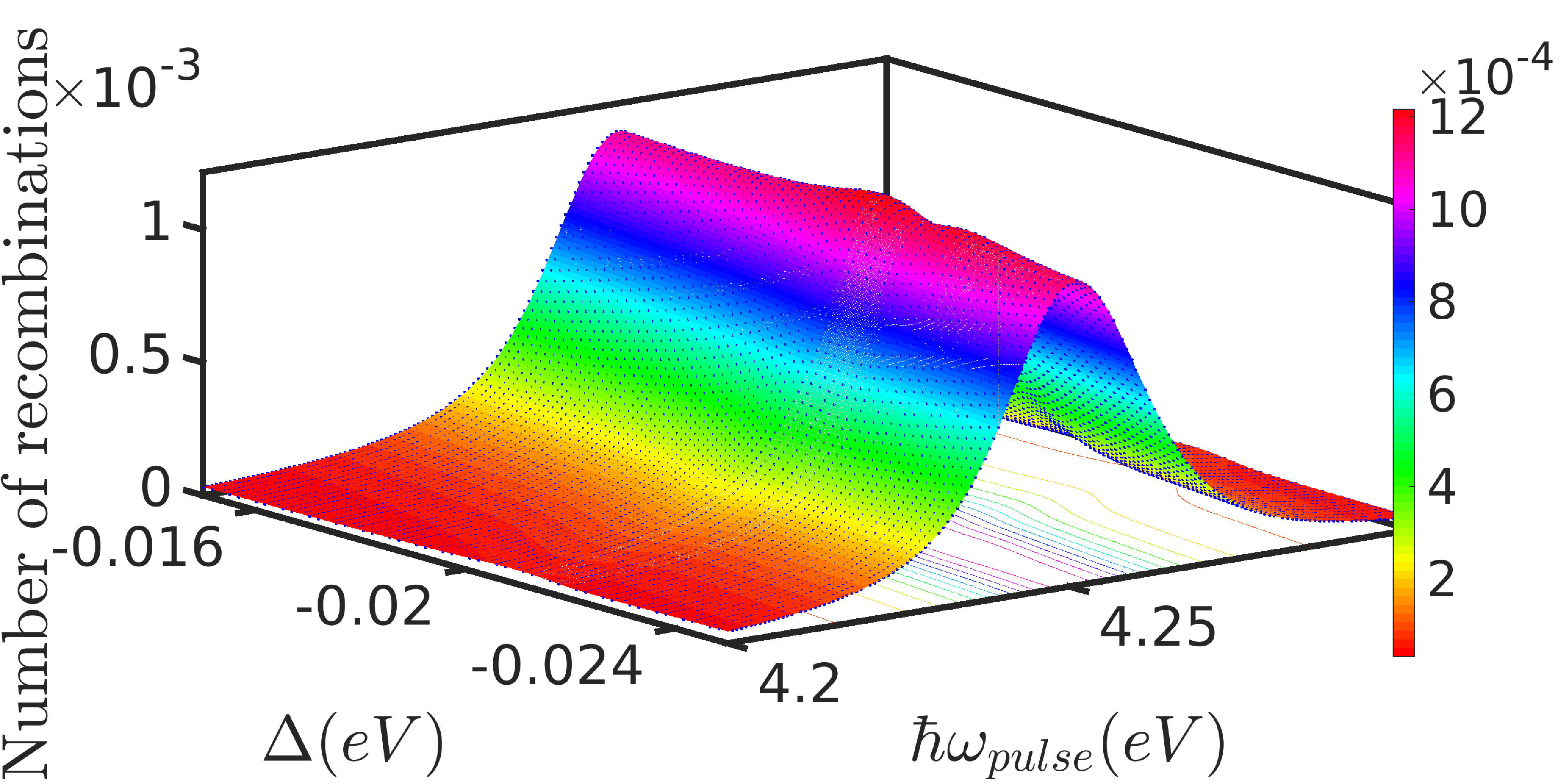
(a) Calculated number of recombinations

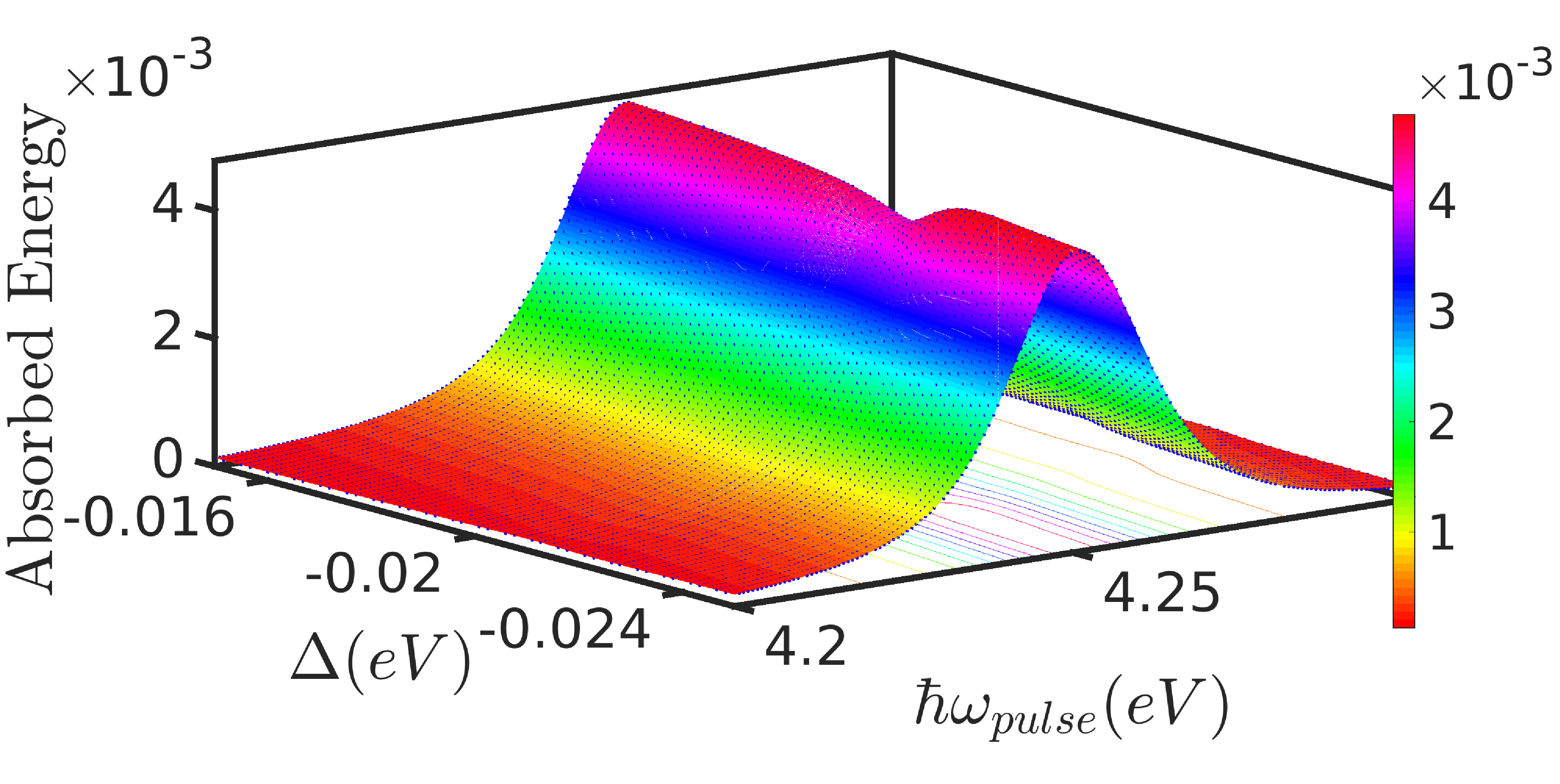
(b) Calculated absorbed energy

Figure 2: Calculated number of recombinations (a) and absorbed energy (b) as a function of $\Delta$ and pulse frequency close to the transition between the 2p states. The pulse area is $\Theta=0.035\pi$.

The yield is then defined as the ratio between the number of recombinations and the absorbed photons. The latter is given by the absorbed energy divided by the photon energy. Due to the short pulse width the photon energy is not well defined. Thus we take the energy $\hbar\omega_{\rm pulse}$, where the number of recombinations peaks for a given detuning $\Delta$. The corresponding result is plotted in Fig. 3

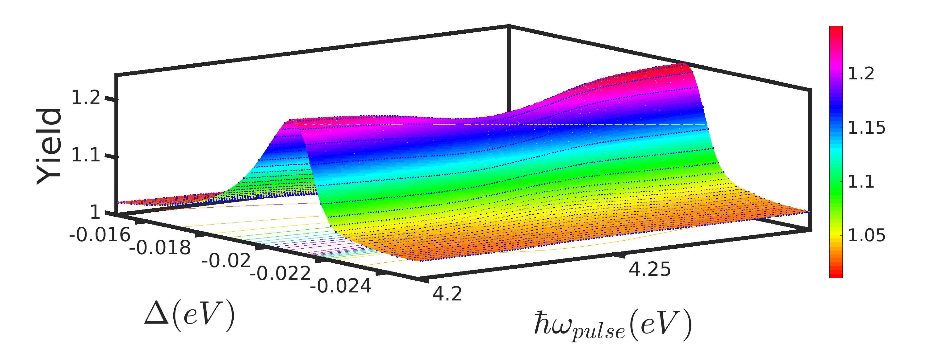
Figure 3: Quantum yield combining the data of Figs. 2(a,b)

We observe a quantum yield of $\approx 1.2$ close to resonance $\Delta\approx-0.0215$ eV. This yield agrees well with the experimentally observed values in these dots reported by Karki et al.[9]. However we obtain this number only for a specific type of dots, characterised by our phenomenological parameter $\Delta$.

Now we want to study the kinetics in detail for $\Delta=-0.0215$ eV, where the single exciton and double exciton states are very close in energy. Thus, the states $|SX\rangle$ and $|DX\rangle$ mix significantly, which results in the singlet states $|22\rangle$ and $|26\rangle$ in our many-body calculation. Analysing these states they can be decomposed as

$$|22\rangle\approx\alpha_{1}|SX\rangle+\beta_{1}|DX\rangle$$ (19)

and

$$|26\rangle\approx\alpha_{2}|SX\rangle+\beta_{2}|DX\rangle$$ (20)

where further contributions are neglected. In terms of these coefficients the probability for the double exciton and single exciton is given by

$$\begin{split}&\rho_{\mathrm{DX,DX}}=\langle DX|\rho|DX\rangle=\alpha^{2}_{1}\rho_{26,26}+\alpha^{2}_{2}\rho_{22,22}-2\alpha_{1}\alpha_{2}\Re\{\rho_{22,26}\}\\ \end{split}$$ (21)

$$\begin{split}&\rho_{SX,SX}=\langle SE|\rho|SX\rangle=\beta^{2}_{1}\rho_{26,26}+\beta^{2}_{2}\rho_{22,22}-2\beta_{1}\beta_{2}\Re\{\rho_{22,26}\}\\ \end{split}$$ (22)

respectively where $\Re$ denote the real part of the coherences between the states $|22\rangle$ and $|26\rangle$.

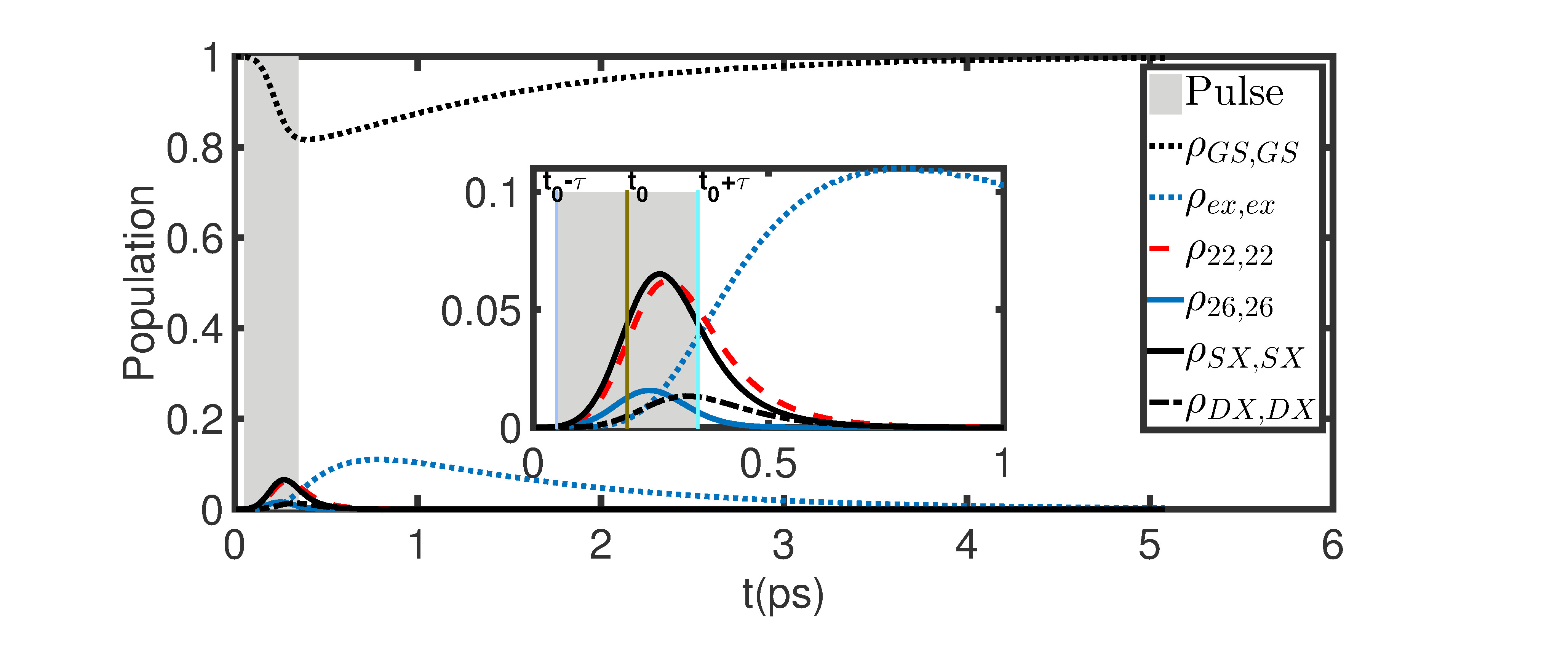
Figure 4: Time evolution for selected many particle states for $\Delta=-0.0215$ eV , $\hbar\omega_{\mathrm{pulse}}=4.255$ eV. An increased pulse area of $\Theta=\pi/2$ is used in order to emphasise the effect. The grey area depicts the duration of the pulse. The inset is an enlargement for small times.

Fig. 4 shows the time evolution of some selected many-particle states when the two excitons are close and a pulse in resonance with the state $|SX\rangle$ is used. In the region where the pulse is active, coherent population transfer is dominating mechanism. It can be seen that for a strong pulse $\Theta=\pi/2$ the system is excited significantly. The $|SX\rangle$ state is the first to be excited as the pulse is tuned to be in resonance with this state and the transition is optically allowed. Subsequently (around $t_{0}$) the state $|DX\rangle$ starts to grow, which can be understood as impact ionisation due to the Coulomb interaction sketched in Fig. 1(a). Almost at the same time, the single exciton ground states $|ex\rangle$ starts growing as it is fed by relaxation processes from the excited exciton $|SX\rangle$ via intermediate states not plotted here. Finally, the $|SX\rangle$ and $|DX\rangle$ states lose their population after the pulse due to the slow recombination rate. In addition there is an Auger contribution, where $|DX\rangle$ is transferred back to $|SX\rangle$.

Within the many-body eigenstates, the same story is told differently: The optically excited state $|SX\rangle$ is a linear combination of $|22\rangle$ and $|26\rangle$. Thus the population of these two states is evolving in parallel. However, due to the energy splitting $\Delta\geq 2V_{DX,SX}$, the coherence $\rho_{22,26}$ is oscillating in time with the angular frequency $\Delta/\hbar$. Eqs. (LABEL:Eq:rho_DX,LABEL:Eq:rho_SX) show that this oscillation implies population changes in $|SX\rangle$ and $|DX\rangle$. Relaxation processes reduce the populations of $|SX\rangle$ and $|DX\rangle$ slightly after the peak of the pulse at $t_{0}=0.2$ ps was reached and the generation becomes weaker. Due to this relaxation and, equally important, dephasing, the oscillation period is never completed for the parameters used.

4 Conclusion and outlook

In this work, we have studied MEG due to optical excitations in $4$ nm PbS quantum dots. We took into account the electron-electron interaction by diagonalising the Hamiltonian. In this basis we solved the equation of motion for the density matrix in the Lindblad form. We find a yield of $1.2$ for a $\hbar\omega_{\rm pulse}\approx 4.2$ eV. This goes well with the experimental observation of a yield of $1.2$ for photon energies surpassing 3 times the lowest exciton absorption [9]. Furthermore, we clarified the relation between the picture of impact-ionisation and a description with diagonal many-particle states.

While the values of the yield are promising, it is not clear, why these values for a particular range of parameters $\Delta$ are representative for the actual experiment. One might argue that the multitude of many-particle states arising if further single-particle levels are taken into account for, offers a plentitude of such resonances, so that they become generic similar to the scenario discussed for tunneling in [29]. This has, however, to be studied further in detail. Another interesting point for further study is the optimisation of the yield and the harvesting of multiple excitons by appropriate contacts. To be able to benefit from MEG, an efficient extraction mechanism is a key. One promising demonstration of efficiently collecting the multiple excitons produced is by Sambur et al. [30] in which they attached a single layer of PbS quantum dot to a thin oxide ($TiO_{2}$). They claim that the strong electronic coupling and favorable energy level alignment between the quantum dot and the oxide facilitates a quick extraction of multiple excitons before they recombine. This can actually be quantified using an extension of the model used here. Corresponding work is ongoing.

5 Acknowledgements

We thank Tönu Pullerits and Khadga Karki for helpful discussions and the Knut and Alice Wallenberg foundation as well as NanoLund for financial support.

6 References

References

- [1] Beard M C 2011 J. Phys. Chem. Lett. 2 1282
- [2] Nozik A J 2008 Chemical Physics Letters 457 3
- [3] Shabaev A, Efros A L and Nozik A J 2006 Nano Letters 6 2856
- [4] Schaller R D and Klimov V I 2004 Phys. Rev. Lett. 92 186601
- [5] Beard M C, Midgett A G, Hanna M C, Luther J M, Hughes B K and Nozik A J 2010 Nano Letters 10 3019
- [6] Klimov V I 2007 Annu. Rev. Phys. Chem. 58 635
- [7] Wise F W 2000 Accounts of Chemical Research 33 773–780
- [8] Kang I and Wise F W 1997 J. Opt. Soc. Am. B 14 1632
- [9] Karki K J, Ma F, Zheng K, Zidek K, Mousa A, Abdellah M A, Messing M E, Wallenberg L R, Yartsev A and Pullerits T 2013 Scientific Reports 3 2287
- [10] Schaller R D, Petruska M A and Klimov V I 2005 Applied Physics Letters 87 253102
- [11] Gachet D, Avidan A, Pinkas I and Oron D 2010 Nano Letters 10 164
- [12] J J H Pijpers, E Hendry, M T W Milder, R Fanciulli, J Savolainen, J L Herek, D Vanmaekelbergh, S Ruhman, D Mocatta, D Oron, A Aharoni , U Banin, and Bonn M 2007 The Journal of Physical Chemistry C 111 4146
- [13] Stubbs S K, Hardman S J O, Graham D M, Spencer B F, Flavell W R, Glarvey P, Masala O, Pickett N L and Binks D J 2010 Phys. Rev. B 81 081303
- [14] Matthew C Beard, Kelly P Knutsen, Pingrong Yu, Joseph M Luther, Qing Song, Wyatt K Metzger, Randy J Ellingson, and Arthur J Nozik 2007 Nano Letters 7 2506
- [15] Smith C and Binks D 2013 Nanomaterials 4 19
- [16] Klimov V I, Mikhailovsky A A, McBranch D W, Leatherdale C A and Bawendi M G 2000 Science 287 1011
- [17] Crooker S A, Barrick T, Hollingsworth J A and Klimov V I 2003 Applied Physics Letters 82
- [18] Träger F 2007 Springer handbook of lasers and optics (Springer Science & Business Media)
- [19] Choi Y, Sim S, Lim S C, Lee Y H and Choi H 2013 Scientific Reports 3 3206
- [20] Semonin O E, Luther J M, Choi S, Chen H Y, Gao J, Nozik A J and Beard M C 2011 Science 334 1530
- [21] Allan G and Delerue C 2006 Phys. Rev. B 73 205423
- [22] Schulze F, Schoth M, Woggon U, Knorr A and Weber C 2011 Phys. Rev. B 84 125318
- [23] Azizi M and Machnikowski P 2013 Phys. Rev. B 88 115303
- [24] O Madelung U Rössler M S 1998 Lead sulfide (pbs) optical properties, dielectric constants Landolt-Börnstein, Group III Condensed Matter vol 41C (Springer-Verlag)
- [25] Sirtori C, Capasso F, Faist J and Scandolo S 1994 Phys. Rev. B 50 8663
- [26] Davies J H 1997 The physics of low-dimensional semiconductors: an introduction (Cambridge university press)
- [27] Mukamel S 1995 Principles of nonlinear optical spectroscopy (Oxford University Press)
- [28] Lindblad G 1976 Comm. Math. Phys. 48 119
- [29] Goldozian B, Damtie F A and Wacker A 2015 preprint arXiv:1501.02974
- [30] J B Sambur, T Novet and B A Parkinson 2010 Sciences 330 63
- [31] J M An, A Franceschetti, S V Dudiy and A Zunger 2006 Nano Letters 6 2728