Dynamics of a Qubit in a High-Impedance Transmission Line from a Bath Perspective

Abstract

We investigate the quantum dynamics of a generic model of light-matter interaction in the context of high impedance waveguides, focusing on the behavior of the photonic states generated in the waveguide. The model treated consists simply of a two-level system coupled to a bosonic bath (the ohmic spin-boson model). Quantum quenches as well as scattering of an incident coherent pulse are studied using two complementary methods. First, we develop an approximate ansatz for the electromagnetic waves based on a single multimode coherent state wavefunction; formally, this approach combines in a single framework ideas from adiabatic renormalization, the Born-Markov approximation, and input-output theory. Second, we present numerically exact results for scattering of a weak intensity pulse by using Numerical Renormalization Group (NRG) calculations. NRG provides a benchmark for any linear response property throughout the ultra-strong coupling regime. We find that in a sudden quantum quench, the coherent state approach produces physical artifacts, such as improper relaxation to the steady state. These previously unnoticed problems are related to the simplified form of the ansatz that generates spurious correlations within the bath. In the scattering problem, NRG is used to find the transmission and reflection of a single photon, as well as the inelastic scattering of that single photon. Simple analytical formulas are established and tested against the NRG data that predict quantitatively the transport coefficients for up to moderate environmental impedance. These formulas resolve pending issues regarding the presence of inelastic losses in the spin-boson model near absorption resonances, and could be used for comparison to experiments in Josephson waveguide quantum electrodynamics (QED). Finally, the scattering results using the coherent state wavefunction approach are compared favorably to the NRG results for very weak incident intensity. We end our study by presenting results at higher power where the response of the system is nonlinear.

I Introduction

Quantum optics deals with the interaction of matter and electromagnetic waves in regimes where the granularity of light comes into play. Typically, because both the fine structure constant and atomic dipoles are small, matter-light coupling is weak, allowing treatment by simple and controlled methodologies, such as the rotating wave approximation (RWA), Born-Markov schemes, and Fock space truncation Sargent . However, recent artificial systems such as superconducting waveguides Niemczyk ; Forn ; Astafiev ; Abdumalikov ; Hoi ; vanLoo , especially the ones using Josephson junction elements to boost the circuit impedance  Masluk ; Bell ; Altimiras ; Weissl ; LeHur , constitute metamaterials where charge density fluctuations mimic an optical-like medium in which the coupling to matter (namely superconducting qubits) can be ultra strong. In this situation, a plethora of interesting phenomena, such as wide-band frequency conversion Goldstein , large non-linearities Peropadre , and non-trivial many-body vacua Goldstein ; Snyman1 , have been theoretically predicted.

In this context, the standard theoretical approaches mentioned above are insufficient: Born-Markov schemes are clearly violated by the large coupling constant, and counter-rotating terms cannot be neglected anymore. In addition, a brute force Fock truncation of the full Hilbert space becomes numerically prohibitive due to the large number of photons generated in the environment, unless one can target physical states using an optimal variational basis, such as matrix product states (MPS) Guo ; Zueco ; Bruognolo ; Chin ; PichlerZoler or within the systematic coherent state expansion (CSE) pioneered in Ref. Bera1, and susequently extended to a variety of dissipative models Bera2 ; ZhaoSubohmic ; ZhaoTwobath ; Snyman2 .

In this article, we probe the idea that multi-mode coherent states are a well-adapted tool to deal with ultra-strong coupling quantum optics by investigating in depth several dynamical properties that are experimentally relevant, such as population decay, coherence buildup, and photon scattering in a large-impedance superconducting waveguide. Historically, this approximate single-coherent state approach was devised for the ground state of the spin-boson model by Luther and Emery EmeryLuther and subsequently by Silbey and Harris Silbey ; Harris and other authors ChinSubohmic ; Nazir , before the demonstration that it can be turned into a systematic expansion that allows one to reach the exact many-body ground state for any coupling strength Bera1 ; Bera2 ; Snyman2 and an arbitrary bath spectral density ZhaoSubohmic . Starting down this same route, we study quantum dynamics here only at the simplest Silbey-Harris level, thus using a single variational coherent state as a lowest order approximation for the time-dependent problem (this is also called the Davidov ansatz). Such an approach has been previously applied to study quantum dynamics for a variety of physical problems Zhao1 ; Zhao2 ; Skrinjar ; Zhao3 ; BeraPV , and it can be adapted to address scattering of Fock states Bermudez . The present study allows us to thoroughly assess the merits and drawbacks of this very economical approach; the numerically-exact full generalization of the systematic CSE to the time domain will be addressed in subsequent work.

We will demonstrate here that this simple-minded single coherent state approach already contains most of the physics at play and naturally bridges from the weak to ultra-strong coupling regimes. Indeed, population decay is found to cross over from underdamped to overdamped relaxation at increasing environmental impedance, as expected physically Leggett ; Weiss . In addition, this single-coherent state approximation predicts elastic transmission lineshapes beyond the RWA that in the linear response regime match precisely our non-perturbative calculations using the Numerical Renormalization Group (NRG). These simulations are used to derive simple and accurate analytical formulas for the transmission coefficients and total inelastic deficits, that can then be used to compare to experiments in waveguide QED.

However, we point out some shortcomings of the single coherent state dynamics that were not reported so far in the literature. Artifacts are indeed generically found whenever the two-level system is subject to a strong temporal perturbation, such as a quantum quench or a strong irradiation pulse (beyond the linear response regime). In all these cases, relaxation is found towards an incorrect steady state where long range correlations are spuriously maintained between the two-level system and modes propagating away from it. These artifacts are a consequence of the constrained form of the single coherent state ansatz, which neglects entanglement within the bath states at all times, and are likely to be cured by extending the present technique to a dynamical version of the systematic coherent state expansion Bera1 ; Bera2 .

The paper is structured as follows. In Sec. II we introduce the spin-boson model and establish the dynamical equations based on the single coherent state ansatz. Then, in Sec. III we study a simple quantum quench where the two-level system is subject to the temporal oscillation of a polarization field. We show that the population decays as physically expected, with a crossover from underdamped to overdamped behavior at increasing coupling strength. However, the dynamics of the quantum coherences is incorrect: it builds up to a value that does not match the expected steady state. We relate this to artifacts in the bath dynamics. When the switching of the perturbation is made adiabatic, however, proper relaxation is finally recovered, a behavior that we relate to a factorization property of the emitted wavepacket. A different physical setup is then considered in Secs. IV and V, whereupon the environment subjects the two-level system to a train of incoming photons. Transport coefficients are extracted from the quantum dynamics and compared favorably to NRG calculations. Simple and accurate formulas are also extracted from these simulations. Some perspectives are given as a conclusion to the paper.

II Single coherent state dynamics

II.1 Model

We start with the standard spin-boson model Leggett ; Weiss , where a two-level system (for instance, a superconducting qubit in the context of circuit QED) is coupled to a set of quantized harmonic oscillators describing propagating modes in a transmission waveguide. We assume in what follows a geometry where the qubit is side-coupled to the waveguide, but our results can be straightforwardly extended to the case of inline coupling. The initial Hamiltonian reads:

$$H=\frac{\Delta}{2}\sigma_{x}-\frac{\sigma_{z}}{2}\sum_{k\in\mathbb{R}}g_{k}(a^{\phantom{e\dagger}}_{k}+a^{\dagger}_{k})+\sum_{k\in\mathbb{R}}\omega_{k}a^{\dagger}_{k}a^{\phantom{e\dagger}}_{k}.$$ (1)

Here $\Delta$ is the splitting of the two-level system (typically set by the Josephson energy associated with the superconducting qubit). We will take a linear relation $\omega_{k}=|k|$, where $k$ is the momentum, setting the plasmon velocity to unity. Finally, we parametrize the coupling constant as $g_{k}=\sqrt{2\alpha|k|}\theta(\omega_{c}-\omega_{k})$. These assumptions accurately describe superconducting waveguides at characteristic energies that are well below the cutoff frequency $\omega_{c}$. As a result, the spectral density in the continuum limit reads $J(\omega)=\sum_{k>0}\pi g_{k}^{2}\delta(\omega-\omega_{k})=2\pi\alpha\,\omega\,\theta(\omega_{c}-\omega)$, where, in case of electric coupling, the dimensionless coupling strength $\alpha$ is proportional to the impedance of the waveguide. As is standard practice, it is useful to fold the problem onto a half-line, by defining even and odd modes,

$$a_{k}^{e}=\frac{1}{\sqrt{2}}\left(a_{k}+a_{-k}\right)\quad\textrm{and}\quad a_{k}^{o}=\frac{1}{\sqrt{2}}\left(a_{k}-a_{-k}\right),$$ (2)

so that the Hamiltonian (1) can be rewritten:

$$H=\frac{\Delta}{2}\sigma_{x}-\frac{\sigma_{z}}{2}\sum_{k>0}g_{k}(a^{e\phantom{\dagger}}_{k}+a^{e\dagger}_{k})+\sum_{k>0}\omega_{k}[a^{e\dagger}_{k}a^{e\phantom{\dagger}}_{k}\!+a^{o\dagger}_{k}a^{o\phantom{\dagger}}_{k}].$$ (3)

II.2 Dynamical ansatz and quantum equations of motion

In the small impedance limit, $\alpha\ll 1$, it is customary to invoke the rotating wave approximation (RWA) Sargent , where Hamiltonian (3) is truncated such that qubit levels dressed only by adjacent Fock states are included. However, this approximation breaks down already for $\alpha\gtrsim 0.1$, and so for our purposes the model must be addressed in its full complexity. A particular defect of the RWA is the lack of many-body renormalization—that is, the strong reduction of the bare tunneling energy $\Delta$ to a smaller value $\Delta_{R}$. This renormalization effect is, however, well-described by an alternative approach, where the dressing of the qubit levels occurs via coherent states EmeryLuther ; Silbey ; Harris ; Nazir ; Bera1 . At the lowest degree of approximation, a single multimode coherent state is introduced for each qubit state, so that the time-dependent state vector takes the form of the following simple ansatz:

$$\left|\Psi(t)\right\rangle = p(t)\left|\uparrow\right\rangle e^{\sum_{k}[f_{k}(t)a^{e\dagger}_{k}-f_{k}^{*}(t)a^{e\phantom{\dagger}}_{k}]}\left|0\right\rangle$$

$$+q(t)\left|\downarrow\right\rangle e^{\sum_{k}[h_{k}(t)a^{e\dagger}_{k}-h_{h}^{*}(t)a^{e\phantom{\dagger}}_{k}]}\left|0\right\rangle.$$

Here $p(t)$ and $q(t)$ are the time-dependent amplitudes of the dressed qubit states (and map the entire Bloch sphere), while $f_{k}(t)$ and $h_{k}(t)$ denote complex displacements of the associated bath oscillators dressing the qubit. The bath states assume thus a simplified form, where entanglement between the various modes is simply neglected. As a particular case, note that the approximate Silbey-Harris state that is obtained for the ground state of Hamiltonian (3) satisfies the relations (obtained by energy minimization) $p=-q=1/\sqrt{2}$, $f_{k}=-h_{k}\equiv f_{k}^{\mathrm{SH}}=(1/2)g_{k}/(\omega_{k}+\Delta_{R})$, where $\Delta_{R}$ is the renormalized qubit tunnel amplitude, an important parameter in what follows.

Only the even modes of the waveguide appear in the ansatz (II.2) as the odd modes are decoupled from the qubit. In Section III, the odd modes will be taken in their vacuum state and will not be considered in the dynamics. However, the transport conditions considered in Sec. V will require inclusion of the odd modes, which is trivially done since their evolution is given by the free part of Hamiltonian (3).

The quantum dynamics will be piloted by the real Langrangian density $\mathcal{L}=\big{<}\Psi(t)|\frac{i}{2}\overrightarrow{\partial_{t}}-\frac{i}{2}\overleftarrow{\partial_{t}}-\mathcal{H}|\Psi(t)\big{>}$, with Euler-Lagrange type of equations of motion, as resulting from the Dirac-Frenkel time-dependent variational principle Saraceno :

$$\frac{d}{dt}\frac{\partial\mathcal{L}}{\partial\dot{f}_{k}}=\frac{\partial\mathcal{L}}{\partial f_{k}},\;\frac{d}{dt}\frac{\partial\mathcal{L}}{\partial\dot{h}_{k}}=\frac{\partial\mathcal{L}}{\partial h_{k}},\;\frac{d}{dt}\frac{\partial\mathcal{L}}{\partial\dot{p}}=\frac{\partial\mathcal{L}}{\partial p},\;\frac{d}{dt}\frac{\partial\mathcal{L}}{\partial\dot{q}}=\frac{\partial\mathcal{L}}{\partial q}.$$

This results in the set of dynamical equations:

$$i\dot{f}_{k} = \omega_{k}f_{k}-\frac{g_{k}}{2}-\frac{q\Delta}{2p}(f_{k}-h_{k})\left\langle f|h\right\rangle,$$ (6)

$$i\dot{h}_{k} = \omega_{k}h_{k}+\frac{g_{k}}{2}-\frac{p\Delta}{2q}(h_{k}-f_{k})\left\langle h|f\right\rangle,$$ (7)

$$i\dot{p} = \frac{\Delta}{2}q\left\langle f|h\right\rangle-p\sum_{k}\frac{g_{k}}{4}(f_{k}+f_{k}^{*})+p\sum_{k}\omega_{k}|f_{k}|^{2}$$ (8)

$$-i\frac{p}{2}\sum[\dot{f}_{k}f_{k}^{*}-\dot{f}_{k}^{*}f_{k}],$$

$$i\dot{q} = \frac{\Delta}{2}p\left\langle h|f\right\rangle+q\sum_{k}\frac{g_{k}}{4}(h_{k}+h_{k}^{*})+q\sum_{k}\omega_{k}|h_{k}|^{2}$$ (9)

$$-i\frac{q}{2}\sum[\dot{h}_{k}h_{k}^{*}-\dot{h}_{k}^{*}h_{k}],$$

where $\left\langle f|h\right\rangle=e^{\sum_{k}[f_{k}^{*}h_{h}-|f_{k}|^{2}/2-|h_{k}|^{2}/2]}$. In practice, Eqs. (6-7) are substituted into Eqs. (8-9), so that an independent set of first-order non-linear differential equations is obtained, which can be efficiently solved by standard Runge-Kutta techniques, with a linear scaling of the computational cost in the number of bosonic modes.

Such dynamical equations have a long history from polaron physics Skrinjar ; Zhao3 ; BeraPV to dissipative quantum mechanics Zhao1 ; Zhao2 , and have been previously derived in the literature. Our purpose in this paper is to benchmark carefully the physical results that they lead to, in order to pinpoint the advantages and drawbacks in using them in the specific context of waveguide QED. We first consider in the next section the situation of quantum quenches, before turning to the investigation of scattering properties.

III Population decay and coherence buildup

III.1 Sudden quantum quench

We investigate here a standard protocol, where the qubit is initialized at time $t=0$ in the state $\left|\uparrow\right\rangle$, while the bath is taken in the vacuum $\left|0\right\rangle$. (Note that $\left|\uparrow\right\rangle$ is not the excited state of the qubit but rather a quantum superposition of the ground and excited state.) The qubit then evolves at later times according to the full spin-boson Hamiltonian (3), and progressively relaxes to its many-body ground state while energy is dissipated into the bath. This theoretical problem has been considered by a great variety of methods, such as quantum Monte Carlo Egger ; Ankerhold , stochastic expansions Gisin ; Grabert ; Orth , time-dependent NRG BullaAnders ; Hofstetter , systematic variational dynamics WangThoss , and analytical weak-coupling calculations Schoeller1 ; Kehrein ; Kennes ; Schoeller2 , but mostly from the perspective of the qubit dynamics. Indeed, in addition to the relaxation properties of the qubit itself, we will examine here in depth the behavior of the states in the bath. This joint qubit and bath dynamics is approximated using the simple equations of motion Eqs. (6)-(9), with the initial conditions $p=1$, $q=0$, $f_{k}=h_{k}=0$. In fact, for numerical stability reasons, one must give a small non-zero value, typically $q=10^{-3}$ at initial times.

By symmetry, the two-level system shows no polarization along the $z$-axis in its ground state (this applies only in the delocalized phase $\alpha<1$, otherwise spontaneous polarization does occur). Due to the presence of the transverse field $\Delta$, one expects precession of the spin and so damped oscillation of $P(t)\equiv\left<\sigma_{z}(t)\right>$ reaching zero in the long-time limit. In addition, it is known that the dynamics crosses over from an underdamped to an overdamped regime as dissipation reaches values around $\alpha=0.5$. Finally, one expects the oscillations to occur at a renormalized frequency $\Delta_{R}\simeq\Delta(\Delta/\omega_{c})^{\alpha/(1-\alpha)}$ with a damping rate $\Gamma\simeq\alpha\Delta_{R}$.

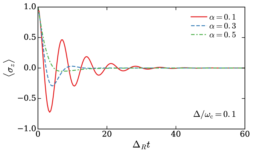
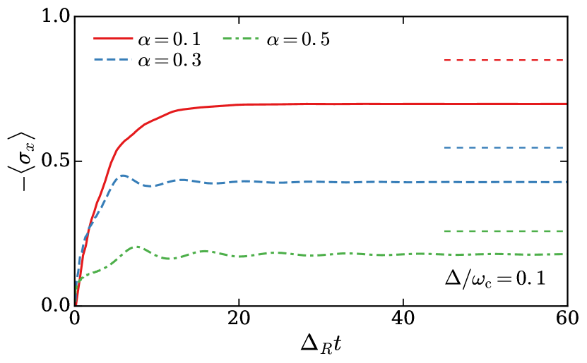
Figure 1: (Color online) Population decay $\big{<}\sigma_{z}(t)\big{>}$ (upper panel) and coherence buildup $\big{<}\sigma_{x}(t)\big{>}$ (lower panel) of the two-level system for several values of dissipation $\alpha=0.1,0.3,0.5$ at $\Delta/\omega_{c}=0.1$. The dashed lines on the vertical axis of the lower panel denote the values for the ground state coherence that are expected from the static single-coherent state approximation. The discrepancy with the long time limit of $\big{<}\sigma_{x}\big{>}$ originates in spurious correlations between the bath and the two-level system.

One remarkable achievement of the single-coherent-state dynamics is that all these non-trivial features of the sudden quench dynamics are qualitatively obtained, as can be seen from the top panel in Fig. 1. Comparison to the existing literature shows however that the precise form of the population decay obtained from this single coherent-state approximation is not fully accurate. First, the exact renormalized qubit splitting differs from the single coherent state result by numerical factors that can be sizable, as was shown recently by extensive CSE calculations in the ground state Bera2 ; Snyman2 . Second, we see that for $\alpha=0.5$, the qubit is still slightly underdamped, while it is known Kennes that the dynamics should be strictly overdamped, without any sign change in $P(t)$.

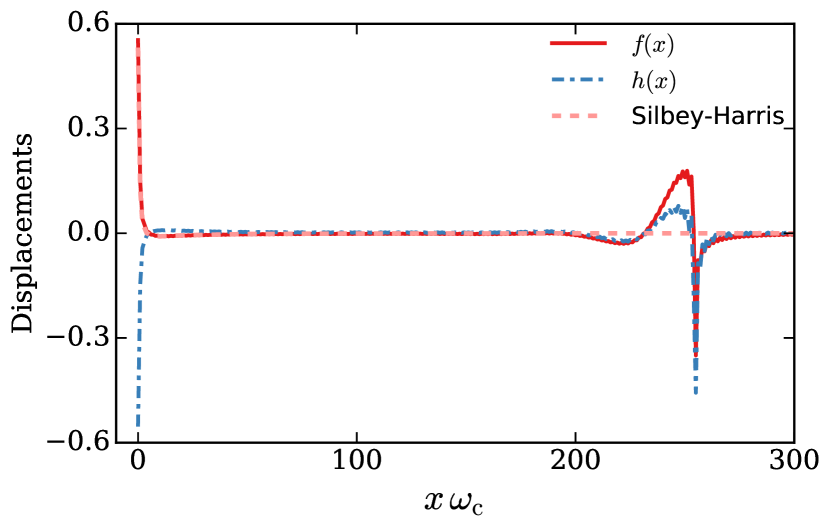
Figure 2: (Color online) Real space displacements $f(x)$ and $h(x)$ associated with the $\uparrow$ and $\downarrow$ components of the wavefunction, respectively, shown for a long time after the instantaneous quench process discussed in the text (parameters are $\Delta=0.1$ and $\alpha=0.2$). At short distances, the Silbey-Harris ground state is stabilized, while at large distances a wavepacket is propagating away from the qubit located at the origin. The lack of factorization, $f(x)\neq g(x)$ for $x>220$, is associated with spurious correlations between the emitted wavepacket and the two-level system, that are responsible for the improper relaxation seen in Fig. 1.

However, a more problematic and qualitative issue arises when monitoring the qubit coherence $\left<\sigma_{x}(t)\right>$, which was not reported in previous studies Zhao1 ; Zhao2 . The lower panel in Fig. 1 shows that the qubit coherence builds as expected qualitatively, but that the long-time limit is in stark disagreement with the value found from the single-coherent-state Silbey-Harris approximation in the ground state Silbey ; Nazir ; Bera1 . Note that the single coherent state ansatz (II.2) captures very precisely the ground state for $\alpha<0.2$, so the discrepancy in the long time value of $\left<\sigma_{x}(t)\right>$ is unexpected. The origin of the problem lies in the states of the bath that carry energy away from the qubit. By monitoring the bath displacements $f_{k}$ and $h_{k}$ in real space (as obtained by Fourier transform), one can see in Fig. 2 that for distances $x\lesssim 1/\Delta_{R}$, an entanglement cloud Snyman1 forms between the qubit and the waveguide, which maps perfectly onto the Silbey-Harris predictions for the ground state (dotted line). This confirms that the origin of the improper relaxation must lie in the propagating waves, that are seen in the plot at larger distances. This can be understood physically in the limit $\alpha\ll 1$ as follows. Let us define the bare qubit ground and excited eigenstates $\left|g\right\rangle=(\left|\uparrow\right\rangle-\left|\downarrow\right\rangle)/\sqrt{2}$ and $\left|e\right\rangle=(\left|\uparrow\right\rangle+\left|\downarrow\right\rangle)/\sqrt{2}$. Our initial state reads: $\left|\Psi(t=0)\right\rangle=\left|\uparrow\right\rangle\otimes\left|0\right\rangle=(1/\sqrt{2})\left|g\right\rangle\otimes\left|0\right\rangle+(1/\sqrt{2})\left|e\right\rangle\otimes\left|0\right\rangle$. At weak dissipation, the configuration $\left|g\right\rangle\otimes\left|0\right\rangle$ is close to the actual ground state, and does dot experience any time evolution. In contrast, the excited state $\left|e\right\rangle\otimes\left|0\right\rangle$ will decay towards the low energy state of the qubit Sargent while emitting a single photon at the resonant frequency $\omega=\Delta$. Thus the complete wavefunction in the long time limit should read:

$$\left|\Psi(t=\infty)\right\rangle = \frac{1}{\sqrt{2}}\left|g\right\rangle\otimes\left|0\right\rangle+\frac{1}{\sqrt{2}}\left|g\right\rangle\otimes a^{\dagger}_{\Delta}\left|0\right\rangle$$ (10)

$$= \frac{(\left|\uparrow\right\rangle-\left|\downarrow\right\rangle)}{\sqrt{2}}\otimes\frac{\left|0\right\rangle+a^{\dagger}_{\Delta}\left|0\right\rangle}{\sqrt{2}}.$$ (11)

Clearly the qubit states and the emitted photons are unentangled in the long time limit, which is in contrast to the outcome of the single coherent state approximation. Indeed, from Fig. 2, one sees that the real space displacements $f(x)$ and $h(x)$ are close to each other, but not strictly equal. This generates some spurious correlations with the qubit states, hence the improper value for the long-time coherence.

III.2 Adiabatic switching

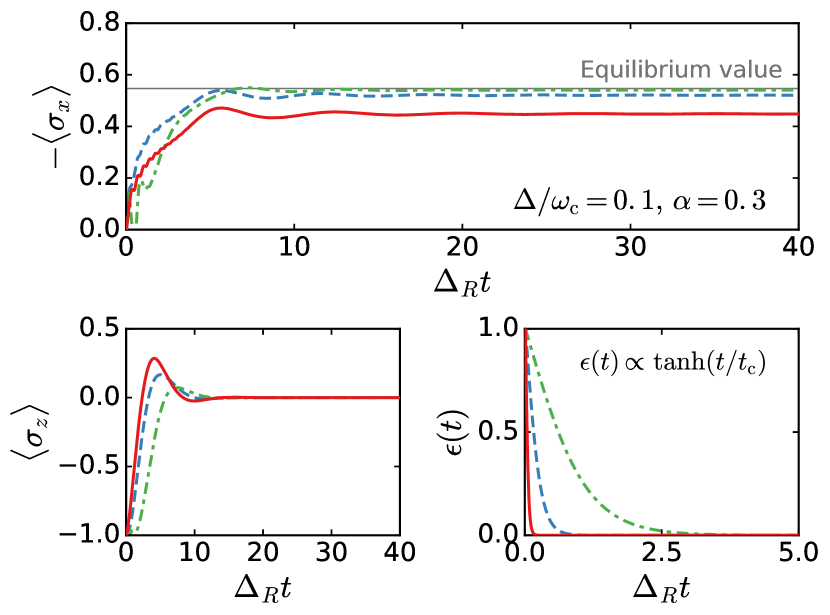
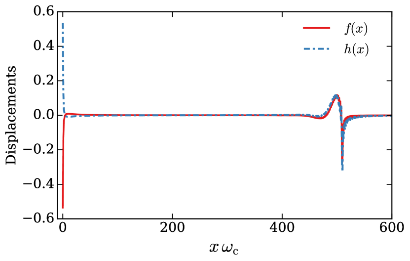
Figure 3: (Color online) Top panel: Coherence $\big{<}\sigma_{x}(t)\big{>}$ as a function of time for three different switching processes (from sudden to adiabatic), that are given by the temporal profile of the local field shown in the rightmost middle panel. The saturation to the equilibrium value is obtained for an adiabatic switching, while the sudden quench shows improper relaxation. The leftmost middle panels shows the associated population decay $\big{<}\sigma_{z}(t)\big{>}$. Bottom panel: real space displacement $f(x)$ and $h(x)$, associated to the $\uparrow$ and $\downarrow$ components of the wavefunction respectively, shown for a long time after the adiabatic quench. Now factorization is correctly recovered, in agreement with the proper relaxation value of $\big{<}\sigma_{x}(t)\big{>}$ at long times.

These moderate artifacts, which are found in previous out-of-equilibrium NRG calculations as well Nghiem , are related to the sudden form of the quench. Indeed, if the qubit is driven adiabatically, the correct relaxation occurs within the single coherent-state scheme. To show this, we still subject the qubit to a time-dependent polarization field $\epsilon(t)$ along the $z$-axis, but now switch it off gradually. The resulting coherence $\left<\sigma_{x}(t)\right>$ is shown in Fig. 3 for three values of the switching time.

For a short switching time, the long-time value of the coherence is underestimated, as for the sudden quenches. However, for a more adiabatic pulse, good convergence towards the ground state value is recovered. At the same time, one can check in Fig. 3 that the emitted wavepacket is factorized with respect to the short distance cloud: indeed, the real space displacements $f(x)$ and $h(x)$ are now equal to each other at large distances, ensuring proper factorization.

These observations thus show the merits and drawbacks of the popular single-coherent-state dynamics, also known as the Davidov dynamical ansatz Zhao1 ; Zhao2 . After a sudden quench, the polarization dynamics and final wavefunction near the origin are captured reasonably well, but the coherence and eventual disentanglement of the qubit and the traveling photon are not. For a sufficiently adiabatic quench, all quantities are correctly captured by the single-coherent-state dynamics.

IV Scattering properties: Numerical renormalization group

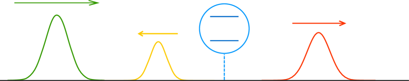
Figure 4: (Color online) Waveguide setup considered here, where a qubit is side-coupled in a two-terminal geometry to a photonic waveguide. Transport properties are described by scattering processes depicted by a set of ingoing and outgoing wavepackets.

In this second part of the paper, we wish to study a typical situation in quantum optics in the specific context of waveguide QED: we investigate the scattering properties of photons in the two-terminal setup depicted in Fig. 4, but in a domain of ultra-strong coupling. This question was investigated by many authors in a regime of weaker coupling, $\alpha\ll 1$, using for instance the RWA Shen ; Zheng ; Wang or extensions to scattering of the Wigner-Weisskopf theory Chen (based on Fock state truncation). In order to tackle the case of large $\alpha$, we first develop a numerically exact approach to the photon scattering properties in the weak intensity limit. This is done by using the numerical renormalization group method Bulla ; Freyn . The results provide an important benchmark for the coherent state dynamics treated in the next section and, indeed, for any calculations of scattering in waveguide QED.

IV.1 Elastic and inelastic transport coefficients from the numerical renormalization group

We start by defining the real-time retarded equilibrium spin susceptibility:

$$\chi(t)=-\frac{i}{4}\theta(t)\left<\mathrm{GS}|[\sigma_{z}(t),\sigma_{z}(0)]|\mathrm{GS}\right>$$ (12)

with $\left|\mathrm{GS}\right>$ the full many-body ground state (note that $\chi(t)$ is a purely real function). Inserting a complete eigenbasis of states $\{\left|a\right\rangle\}$ with respective energies $E_{a}$, one readily obtains:

$$\chi(t)=-\frac{1}{2}\theta(t)\sum_{a}|\left<\mathrm{GS}|\sigma_{z}|a\right>|^{2}\sin[(E_{a}-E_{\mathrm{GS}})t].$$ (13)

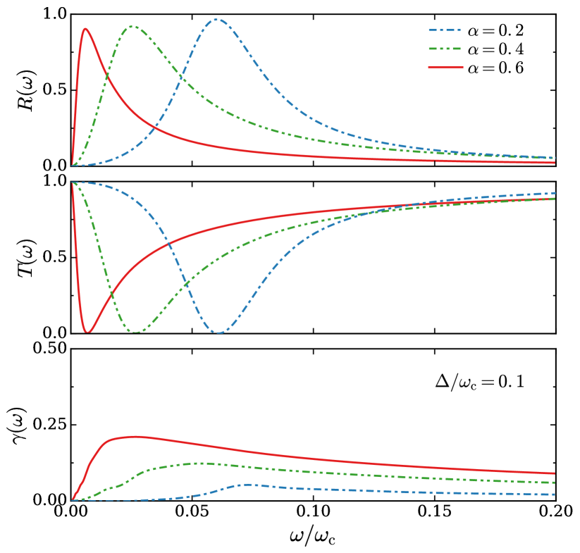
Figure 5: (Color online) Reflection coefficient (top panel), transmission coefficient (middle panel) and total inelastic losses (bottom panel) from the NRG calculations at three values of dissipation $\alpha=0.2,0.4,0.6$ for $\Delta=0.1$. The curves with largest $\alpha$ show a resonant peak at the smallest value of the renormalized qubit splitting $\Delta_{R}$.

This leads to the frequency-resolved spin susceptibility (decomposed into real and imaginary parts):

$$\chi(\omega)\equiv\chi^{\prime}(\omega)+i\chi^{\prime\prime}(\omega)=\int_{-\infty}^{+\infty}\mathrm{d}t\;e^{i\omega t}\chi(t).$$ (14)

In particular, in terms of the Lehman spectral decomposition onto the complete eigenbasis, the imaginary part reads:

$$\chi^{\prime\prime}(\omega) = \frac{\pi}{4}\sum_{a}|\left<\mathrm{GS}|\sigma_{z}|a\right>|^{2}\left[\delta(\omega+E_{a}-E_{\mathrm{GS}})\right.$$ (16)

$$-\left.\delta(\omega-E_{a}+E_{\mathrm{GS}})\right].$$

One thus obtains from the above decomposition a sum rule that will be important in what follows:

$$\int_{-\infty}^{+\infty}\!\!\mathrm{d}\omega\;\chi^{\prime\prime}(\omega)\,\mathrm{Sign}(\omega)=\frac{\pi}{2}.$$ (17)

Now, from linear-response theory LeHur ; Goldstein and using an exact identity for the Green funciton of the bosonic modes,

$$G_{kk^{\prime}}(\omega) \equiv \big{<}a_{k}^{\dagger}(\omega)a_{k^{\prime}}^{\phantom{\dagger}}(-\omega)\big{>}$$ (18)

$$= \frac{\delta_{kk^{\prime}}}{\omega-\omega_{k}}+\frac{g_{k}g_{k^{\prime}}\chi(\omega)}{(\omega-\omega_{k})(\omega-\omega_{k^{\prime}})}$$

which relates the scattering matrix to the qubit response, one obtains the reflection and transmission coefficients,

$$R(\omega) = (2\pi\alpha\omega)^{2}|\chi(\omega)|^{2}$$ (19)

$$T(\omega) = (2\pi\alpha\omega)^{2}[\chi^{\prime}(\omega)]^{2}+[1-2\pi\alpha\omega\chi^{\prime\prime}(\omega)]^{2},$$ (20)

as well as the total inelastic deficit,

$$\gamma(\omega)\equiv 1-R(\omega)-T(\omega)=4\pi\alpha\omega\chi^{\prime\prime}(\omega)-2(2\pi\alpha\omega)^{2}|\chi(\omega)|^{2}.$$ (21)

As they are derived from linear response theory, the reflection and transmission probabilities here are those of a single incoming photon.

These quantities are shown in Fig. 5 for increasing values of dissipation. The reflection/transmission coefficient shows as expected a peak/dip at the qubit absorption frequency $\Delta_{R}$, which progressively renormalizes to smaller values as $\alpha$ increases. At the same time, one notes that the peak value in $R(\omega)$ is slightly lower than unity, with a deviation that increases with enhanced dissipation. This is in contrast to the approximate results of Ref. LeHur, but in agreement with exact calculations at the Toulouse point Bulla ; Goldstein , which read:

$$\chi_{\mathrm{Toulouse}}(\omega)=\frac{1}{2\pi\omega}\frac{1}{\omega+i\Gamma}\log(1-2i\omega).$$ (22)

As a consequence, the inelastic deficit becomes more and more important as $\alpha$ grows, due to stronger photon non-linearities, as shown in the bottom panel. One notes in particular that the deficit $\gamma(\omega)$ peaks above $\Delta_{R}$ and shows very long tails, which are reminiscent of the inelastic contribution to scattering for fermionic Kondo impurities Fritz , although the physical quantities do not correspond strictly here. As previously noted by Goldstein et al. Goldstein , the total inelastic losses are quite important at strong dissipation, and reach above 20$\%$ at $\alpha=0.6$. We note in addition a surprising result from the NRG: while the reflection deficit is sizable [for large impedance, typically up to 10% deviation from unitary scattering at the peak value of $R(\omega)$], the transmission deficit is very small—the transmission dip goes to a tiny (yet non-zero) value. It is practically not possible to see this small background in the middle panel of Fig. 5, but one can verify from the exact Toulouse formula at $\alpha=0.5$ that the minimal transmission is of order $10^{-3}$, a very small number to which we cannot give a simple physical interpretation at this stage.

IV.2 Analytical comparisons

We provide here some analytical insights, comparing previously derived theories to our numerical simulations. We also derive new phenomenological formulas that match the NRG results quite well, and that could be used in practice for easier comparisons to experiments. We do not include checks to the exact Toulouse limit Goldstein , as it has been shown earlier Bulla that the NRG reproduces the spin susceptibility quite accurately at $\alpha=0.5$.

First, we compare the NRG data to approximate results based on the rotating wave approximation used routinely in quantum optics Sargent , which leads to the following $t$-matrix for a unidimensional waveguide:

$$t_{\mathrm{RWA}}(\omega)=\frac{\omega-\Delta}{\omega-\Delta+i\Gamma}.$$ (23)

In this approximation, the qubit level is not renormalized, but acquires a lifetime, with a rate $\Gamma\propto\alpha\Delta$. This leads to the reflection and transmission coefficients:

$$\!\!\!\!\!\!R_{\mathrm{RWA}}(\omega) = |1-t_{\mathrm{RWA}}(\omega)|^{2}=\frac{\Gamma^{2}}{(\omega-\Delta)^{2}+\Gamma^{2}}$$ (24)

$$\!\!\!\!\!\!T_{\mathrm{RWA}}(\omega) = |t_{\mathrm{RWA}}(\omega)|^{2}=\frac{(\omega-\Delta)^{2}}{(\omega-\Delta)^{2}+\Gamma^{2}}.$$ (25)

Clearly, scattering is unitary in the RWA, since $R_{\mathrm{RWA}}(\omega)=1-T_{\mathrm{RWA}}(\omega)$. Due to the lack of inelastic effects, the RWA lineshape should become less accurate as dissipation increases. We see indeed sizable deviations when $\alpha>0.1$ in the upper panel of Fig. 6 by a comparison to NRG for the reflection coefficient. Note that we allow here as fitting parameters for the RWA lineshape the renormalized qubit frequency and linewidth, which improves the agreement somewhat artificially.

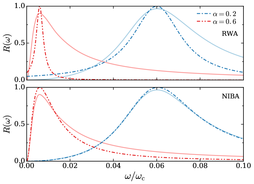
Figure 6: (Color online) Reflection coefficient comparing the RWA Lorentzian lineshape Eq. (24) (dashed lines, upper panel) and the NIBA lineshape Eq. (27) of Ref. LeHur, (dashed lines, lower panel) to the exact NRG calculations (full lines) at two values of dissipation $\alpha=0.2,0.6$ for $\Delta=0.1$. An effective renormalized qubit splitting $\Delta_{R}$ and a renormalized linewidth $\Gamma$ were used as fitting parameters within the RWA and NIBA formulas, for better comparison of the actual lineshapes.

This defect of the RWA has motivated improved perturbative calculations by K. Le Hur LeHur , based on an approximate form for the spin susceptibility that derives from analogy to the Non Interacting Blip Approximation (NIBA) Leggett :

$$\chi_{\mathrm{NIBA}}(\omega)=\frac{\Delta_{R}}{\Delta_{R}^{2}-\omega^{2}-i2\pi\alpha\omega\Delta_{R}}.$$ (26)

From Eqs. (19)-(20), this yields an approximate form of the reflection and transmission coefficients,

$$R_{\mathrm{NIBA}}(\omega) = \frac{(2\Gamma\omega)^{2}}{(\Delta_{R}^{2}-\omega^{2})^{2}+(2\Gamma\omega)^{2}}$$ (27)

$$T_{\mathrm{NIBA}}(\omega) = \frac{(\Delta_{R}^{2}-\omega^{2})^{2}}{(\Delta_{R}^{2}-\omega^{2})^{2}+(2\Gamma\omega)^{2}},$$ (28)

from which the RWA expression (24) is recovered in the limit $\Gamma\ll\Delta_{R}$. These formulas can be seen, however, to again satisfy $R_{\mathrm{NIBA}}(\omega)+T_{\mathrm{NIBA}}(\omega)=1$ and thus miss inelastic losses, as pointed out in Ref. Goldstein, . The comparison to NRG is nevertheless much more satisfactory than with the RWA, as seen in the lower panel of Fig. 6. The only discrepancy comes again from the lack of inelastic contributions within the NIBA expression.

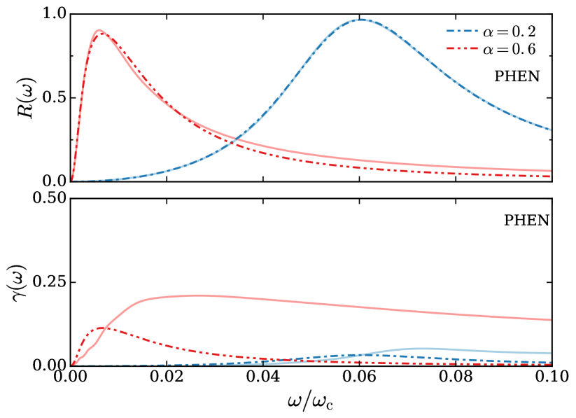
Figure 7: (Color online) Reflection coefficient (top panel) and inelastic deficit (bottom panel) comparing the phenomenological lineshape Eq. (31) (dashed lines) to the exact NRG calculations (full lines) at two values of dissipation $\alpha=0.2,0.6$ (rightmost and leftmost curves respectively). An effective renormalized qubit splitting $\Delta_{R}$ and a renormalized linewidth $\Gamma$ were used as fitting parameters within the phenomenological formula, for better comparison of the actual lineshapes.

The NIBA expression can, in fact, be corrected phenomenologically by noticing a simple problem in the formula for the spin susceptibility (26). Indeed, the sum rule (17) is increasingly violated as $\alpha$ grows:

$$\int_{-\infty}^{+\infty}\!\!\mathrm{d}\omega\;\chi_{\mathrm{NIBA}}^{\prime\prime}(\omega)\mathrm{Sign}(\omega) = \frac{\pi+2\,\mathrm{atan}\left[\frac{2-(2\pi\alpha)^{2}}{2\pi\alpha\sqrt{4-(2\pi\alpha)^{2}}}\right]}{2\sqrt{4-(2\pi\alpha)^{2}}}$$ (29)

$$\equiv \frac{\pi}{2}N_{\alpha}.$$

One recovers $N_{\alpha}\to 1$ for $\alpha\to 0$, but in general the deviation from the sum rule can be large, and, as we will see, accounts for the missing inelastic contribution.

We thus define an improved phenomenological formula:

$$\chi_{\mathrm{phen.}}(\omega)=\frac{1}{N_{\alpha}}\frac{\Delta_{R}}{\Delta_{R}^{2}-\omega^{2}-i2\pi\alpha\omega\Delta_{R}},$$ (30)

which satisfies by construction the exact sum rule. This leads to the following expressions for the reflection, transmission, and inelastic responses:

$$R_{\mathrm{phen.}} = \frac{1}{N_{\alpha}^{2}}\frac{(2\Gamma\omega)^{2}}{(\Delta_{R}^{2}-\omega^{2})^{2}+(2\Gamma\omega)^{2}}$$ (31)

$$T_{\mathrm{phen.}} = \frac{(\Delta_{R}^{2}-\omega^{2})^{2}+(1-N_{\alpha}^{-1})^{2}(2\Gamma\omega)^{2}}{(\Delta_{R}^{2}-\omega^{2})^{2}+(2\Gamma\omega)^{2}}$$ (32)

$$\gamma_{\mathrm{phen.}} = \frac{N_{\alpha}-1}{N_{\alpha}^{2}}\frac{2(2\Gamma\omega)^{2}}{(\Delta_{R}^{2}-\omega^{2})^{2}+(2\Gamma\omega)^{2}}.$$ (33)

The comparison to the NRG data in the top panel of Fig. 7 gives now excellent agreement at $\alpha\leq 0.2$ for the reflection coefficient, and reproduces well the magnitude of the inelastic deficit, although the shift of the peak position and the long tails in $\gamma(\omega)$ are not correctly accounted for. We also see from the bottom panel of Fig. 7 that large deviations occur in $\gamma(\omega)$ for larger $\alpha$ values; this is expected FlorensFritz because a slower decay of the form $\chi^{\prime\prime}(\omega)\sim 1/(\omega\log^{2}\omega)$ is known to occur in the Kondo regime for $\omega\gg\Delta_{R}$. As a result, the inelastic contribution is even more underestimated in this regime.

V Scattering properties: Coherent state dynamics

V.1 Coherent state formalism for a two-terminal waveguide

The problem we want to study is the scattering of a coherent state wavepacket off the Silbey-Harris ground state of the spin-boson model. The strategy is to define the proper initial condition for the wavepacket in left-right space (the full waveguide), then transform it to an even-odd basis, and propagate the resulting state. Since only even modes couple to the qubit, the equations of motion (6)-(9) can be used, while the odd modes are freely propagating. After the scattering process has occured, a transformation back to the left-right basis provides the final wavefunction, which allows one to find the transmitted and reflected intensity.

Mathematically, we denote the initial scattering wavepacket by $z_{x}$ or $z_{k}$ in position space or momentum space, respectively (this excludes the entanglement cloud associated to the Silbey-Harris ground state). These are related by the Fourier transform convention,

$$z_{x}=\int_{-\infty}^{\infty}\frac{dk}{\sqrt{2\pi}}e^{+ikx}z_{k}.$$ (34)

The even and odd parts of the wavepaket are then defined strictly for $k>0$ as

$$z_{k}^{e}=\frac{1}{\sqrt{2}}\left(z_{k}+z_{-k}\right)\quad\textrm{and}\quad z_{k}^{o}=\frac{1}{\sqrt{2}}\left(z_{k}-z_{-k}\right),$$ (35)

which can be inverted to yield

$$z_{k}=\frac{1}{\sqrt{2}}\left(z_{k}^{e}+z_{k}^{o}\right)\quad\textrm{and}\quad z_{-k}=\frac{1}{\sqrt{2}}\left(z_{k}^{e}-z_{k}^{o}\right).$$ (36)

Note that the first expression in Eq. (36) gives the right-going wave ($k>0$), while the second one is the left-going wave ($-k<0$).

We choose to use a Gaussian wavepacket defined as

$$z_{k}=\sqrt{\bar{n}}\left(\frac{1}{2\pi\sigma^{2}}\right)^{\frac{1}{4}}e^{-\frac{(k-k_{0})^{2}}{4\sigma^{2}}}e^{-i(k-k_{0})x_{0}}e^{-ik_{0}x_{0}/2},$$ (37)

corresponding to a signal initially centered around $x_{0}$, with mean wavenumber $k_{0}$, spatial extent $1/\sigma$, and a total intensity corresponding to $\bar{n}$ photons on average. The corresponding real space wavepacket is then

$$z_{x}=\sqrt{\bar{n}}\left(\frac{2\sigma^{2}}{\pi}\right)^{\frac{1}{4}}e^{-(x-x_{0})^{2}\sigma^{2}}e^{+ik_{0}(x-x_{0})}e^{+ik_{0}x_{0}/2}.$$ (38)

Note that these amplitudes are both normalized so that $\int_{-\infty}^{\infty}dx|z_{x}|^{2}=\int_{-\infty}^{\infty}dk|z_{k}|^{2}=\bar{n}$.

Now let us define the actual photon content of the wavepacket, using here coherent states, which are better suited for our simulations than scattering Fock states. The creation operator for a photon in the wavepacket state is defined as

$$a_{z}^{\dagger}=\int_{-\infty}^{+\infty}dk\,z_{k\,}a_{k}^{\dagger}=\int_{-\infty}^{+\infty}dx\,z_{x\,}a_{x}^{\dagger}.$$ (39)

A coherent state with an average of $\bar{n}$ photons in this wavepacket is thus:

$$e^{-\bar{n}/2}e^{a_{z}^{\dagger}}\left|0\right\rangle=e^{a_{z}^{\dagger}-a_{z}}\left|0\right\rangle.$$ (40)

One can construct even and odd creation and destruction operators for bosons in a given mode $k>0$ by analogy to the transformations made previously on the wavepacket:

$$a_{k}^{e}=\frac{1}{\sqrt{2}}\left(a_{k}+a_{-k}\right)\quad\textrm{and}\quad a_{k}^{o}=\frac{1}{\sqrt{2}}\left(a_{k}-a_{-k}\right).$$ (41)

Then the creation operator for the wavepacket state is

$$a_{z}^{\dagger} = \int_{0}^{+\infty}dk\,\left(z_{k\,}a_{k}^{\dagger}+z_{-k\,}a_{-k}^{\dagger}\right)$$ (42)

$$= \int_{0}^{+\infty}dk\,\left(z_{k\,}\frac{a_{k}^{e\dagger}+a_{k}^{o\dagger}}{\sqrt{2}}+z_{-k\,}\frac{a_{k}^{e\dagger}-a_{k}^{o\dagger}}{\sqrt{2}}\right)$$ (43)

$$= \int_{0}^{+\infty}dk\,\left(z_{k\,}^{e}a_{k}^{e\dagger}+z_{k\,}^{o}a_{k}^{o\dagger}\right)=a_{z}^{e\dagger}+a_{z}^{o\dagger}.$$ (44)

Notice that the even and odd sector operators commute,

$$[a_{k}^{e\dagger},a_{k}^{o}]=[a_{z}^{e\dagger},a_{z}^{o}]=0.$$ (45)

Thus, the coherent state wavepacket can finally be written as:

$$e^{-\bar{n}/2}e^{a_{z}^{\dagger}}\left|0\right\rangle=e^{a_{z}^{o\dagger}}e^{-\bar{n}/2}e^{a_{z}^{e\dagger}}\left|0\right\rangle=e^{a_{z}^{o\dagger}}e^{a_{z}^{e\dagger}-a_{z}^{e}}\left|0\right\rangle.$$ (46)

The final step in the initialization of the state vector is to combine the scattering wavepacket coherent state $z_{k}$ with the Silbey-Harris ground state with displacement $f_{k}^{\mathrm{SH}}=(1/2)g_{k}/(\omega_{k}+\Delta_{R})$. Since the even and odd sectors are completely independent, the Silbey-Harris state affects only the even sector. For the spin-up projection of the wavefunction, we have thus,

$$e^{a_{z}^{e\dagger}-a_{z}^{e}}\left|\Psi_{\uparrow}\right\rangle = e^{\sum_{k>0}\left(z_{k}^{e}a_{k}^{e\dagger}-z_{k}^{e*}a_{k}^{e}\right)}$$

$$\times\,e^{\sum_{k>0}\left(f_{k}^{\mathrm{SH}}a_{k}^{e\dagger}-f_{k}^{\mathrm{SH}*}a_{k}^{e}\right)}\left|0\right\rangle,$$

where for compactness we have switched to sums over $k$ instead of integrals. The two exponentials can be combined, keeping in mind that there may be a phase from the commutator in the standard relation $e^{A}e^{B}=e^{A+B}e^{\frac{1}{2}[A,B]}$, which is valid since the commutator here is just a $c$-number. Thus the initial state in the $\uparrow$ projection is

$$e^{a_{z}^{e\dagger}-a_{z}^{e}}\left|\Psi_{\uparrow}\right\rangle = e^{\frac{1}{2}\sum_{k>0}\left(z_{k}^{e}f_{k}^{\mathrm{SH}*}-z_{k}^{e*}f_{k}^{\mathrm{SH}}\right)}$$

$$\times\,e^{\sum_{k>0}\left[\left(f_{k}^{\mathrm{SH}}+z_{k}^{e}\right)a_{k}^{e\dagger}-\left(f_{k}^{\mathrm{SH}}+z_{k}^{e}\right)^{*}a_{k}^{e}\right]}\left|0\right\rangle.$$

For the spin-down projection, one simply replaces $f_{k}^{\mathrm{SH}}$ by $-f_{k}^{\mathrm{SH}}$ without changing the sign of $z_{k}^{e}$, so that our total initial wavefunction reads:

$$\left|\Psi(t=0)\right\rangle = \frac{1}{\sqrt{2}}\left|\uparrow\right\rangle e^{\frac{1}{2}\sum_{k>0}\left(z_{k}^{e}f_{k}^{\mathrm{SH}*}-z_{k}^{e*}f_{k}^{\mathrm{SH}}\right)}$$

$$\times\,e^{\sum_{k>0}\left[\left(f_{k}^{\mathrm{SH}}+z_{k}^{e}\right)a_{k}^{e\dagger}-\left(f_{k}^{\mathrm{SH}}+z_{k}^{e}\right)^{*}a_{k}^{e}\right]}\left|0\right\rangle$$

$$-\frac{1}{\sqrt{2}}\left|\downarrow\right\rangle e^{\frac{1}{2}\sum_{k>0}\left(-z_{k}^{e}f_{k}^{\mathrm{SH}*}+z_{k}^{e*}f_{k}^{\mathrm{SH}}\right)}$$

$$\times\,e^{\sum_{k>0}\left[\left(-f_{k}^{\mathrm{SH}}+z_{k}^{e}\right)a_{k}^{e\dagger}-\left(-f_{k}^{\mathrm{SH}}+z_{k}^{e}\right)^{*}a_{k}^{e}\right]}\left|0\right\rangle.$$

One can thus use this state as initial condition for the equations of motion (6)-(9), with $f_{k}(0)=f_{k}^{\mathrm{SH}}+z_{k}^{e}$, $h_{k}(0)=-f_{k}^{\mathrm{SH}}+z_{k}^{e}$, and $p(0)=-q(0)=1/\sqrt{2}$. Note that the odd sector, which decouples from the qubit, is trivially evolving in time according to $i\dot{z}_{k}^{o}=\omega_{k}z_{k}^{o}$.

After this time-evolution is performed, the output must be analyzed. Because of the constrained ansatz (II.2), the output is again a single coherent state, but one has to recombine the even sector output with the odd sector trivial evolution. After a long enough time $T$ so that the outgoing wavepacket is disentangled from the Silbey-Harris cloud, one obtains the total displacement $f_{k}(T)=f_{k}^{\mathrm{SH}}+z_{k,\mathrm{out}}^{e}$, separating into the ground state contribution and an outgoing scattering part. Combining with $z_{k}^{o}(T)=e^{-i\omega_{k}t}z_{k}^{o}(0)$ using Eq. (36), this provides the final outgoing coherent state displacement $z_{k,\mathrm{out}}$ in the physical momentum basis. One can then define transmission and reflection coefficients as the ratio of the outgoing (in each possible terminal) to the ingoing power:

$$T=\frac{\sum_{k>0}k\left|z_{k,\textrm{out}}\right|^{2}}{\sum_{k>0}k\left|z_{k,i\textrm{n}}\right|^{2}}\quad\textrm{and}\quad R=\frac{\sum_{k<0}|k|\left|z_{k,\textrm{out}}\right|^{2}}{\sum_{k>0}k\left|z_{k,i\textrm{n}}\right|^{2}}.$$ (50)

V.2 Comparison of NRG and coherent state dynamics results for the transport coefficients

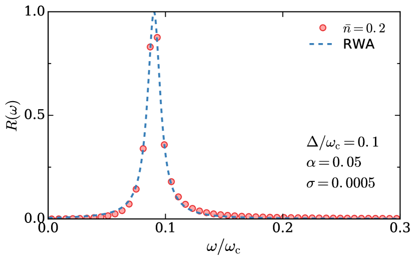
Figure 8: (Color online) In the quantum optics regime $\alpha=0.05$, the reflection coefficient obtained from the variational dynamics (symbols) matches the RWA lineshape (dashed line), which was however corrected with the proper renormalized qubit splitting. Parameters here are $\Delta/\omega_{c}=0.1$ and the variational dynamics is done at weak power ($\bar{n}=0.2$) in order to be in the linear response regime. The wavepacket width is taken very small $\sigma=0.0005$ to allow good spectral resolution.

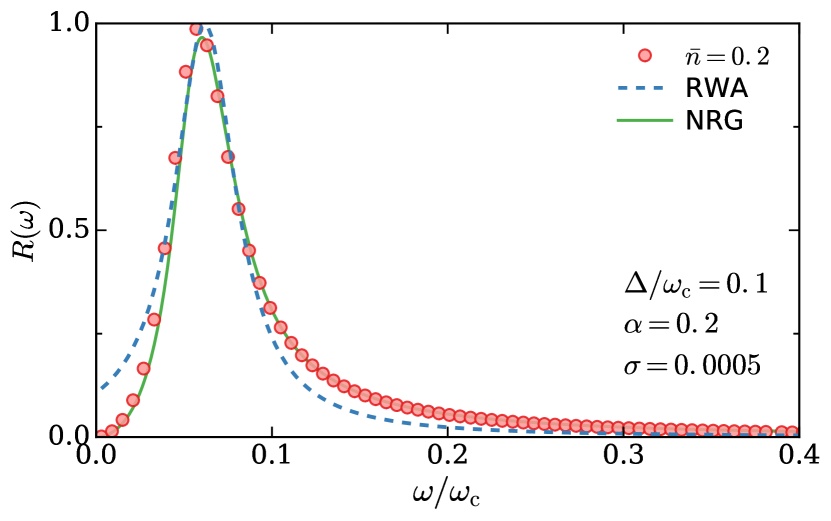
Figure 9: (Color online) In the ultrastrong coupling regime $\alpha=0.2$, the reflection coefficient obtained from the variational dynamics (symbols) compares favorably to the exact NRG lineshape (solid line), while the RWA (dashed line) presents clear deviations. The same parameters as in Fig. 8 were used.

In this last section, we present transport calculations using the single coherent state dynamics and benchmark them in the linear response regime against the controlled results from NRG, including a comparison to RWA as well. Let us first consider the quantum optics regime $\alpha\ll 1$ where the RWA can be trusted, as shown in Fig. 8 for $\alpha=0.05$ and an incident coherent state wavepacket whose intensity is small. We see excellent agreement between the two methods; thus, the coherent state approach performs very well in the quantum optics regime [note that an effective qubit splitting was added by hand in the RWA curve].

Increasing dissipation up to $\alpha=0.2$, we assess the validity of both the coherent state dynamics and the RWA by comparing to the numerically exact NRG results in Fig. 9. While the RWA results are rather inaccurate, the coherent state dynamics is in excellent agreement with the NRG, showing its utility well beyond the usual quantum optics regime.

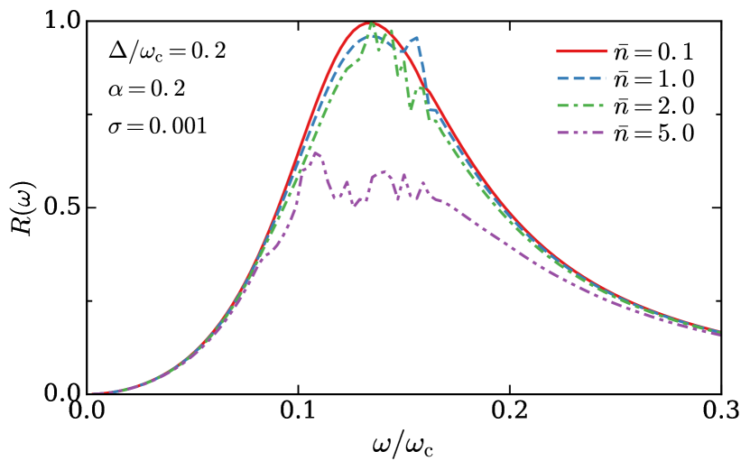
Figure 10: (Color online) Reflection coefficient at $\alpha=0.2$ and $\Delta/\omega_{c}=0.2$ for increasing irradiation power. The incident power is characterized by the average number of photons $\bar{n}$ in the incoming coherent state wavepackets; results for up to $\bar{n}=5$ are shown.

Being a non-equilibrium method, the coherent state dynamics can access regimes beyond linear response, which the present formulation of the NRG is not able to achieve. We show for instance in Fig. 10 how the transport coefficients evolve as input power is turned on, increasing the average number of photons in the incoming coherent state wavepacket up to $\bar{n}=5$. Having checked our numerical integration carefully, we attribute the large level of noise in these results to the restricted form of the ansatz (II.2) and not to numerical inaccuracies. This is consistent with our general observation that artifacts typically arise for strong temporal perturbations in the single coherent state dynamics, which indeed increase at larger power.

The general trend of the curves are however clear LeHur : due to saturation effects of the two-level system by the large flux of photons, the reflection is reduced at increasing power. Clear deviations from the linear response result occur for an average photon number $\bar{n}\simeq 5$. This value can be understood from the fact that the qubit excitation rate $\bar{n}\sigma=5\times 0.005=0.025$ becomes then comparable to the qubit decay rate $\Gamma\simeq\alpha\Delta_{R}=0.2\times 0.15\simeq 0.03$. Saturation effects are indeed expected to be governed by the renormalized qubit frequency at strong coupling.

VI Conclusion

We have investigated here the relaxation and transport properties of a single qubit side-coupled to a large impedance transmission line, using complementary many-body methods. The numerical renormalization group (NRG) allowed us to accurately compute the linear-response transport coefficients, and showed good agreement for a simpler approach using the variational time-evolution of a wavefunction based on a single coherent state. This coherent state dynamics was benchmarked also regarding relaxation properties, and despite some success in predicting the onset of overdamped dynamics, showed some physical artifacts such as improper relaxation to the correct steady state. We plan to overcome these difficulties in future works by systematically extending the dynamical ansatz along the lines of Ref. Bera2 , allowing us also to tackle the transport problem in a more controlled way.

- (1) P. Meystre and M. Sargent, “Elements of quantum optics” (Springer-Verlag Berlin, Heidelberg, 2010).
- (2) T. Niemczyk, F. Deppe, H. Huebl, E. P. Menzel, F. Hocke, M. J. Schwarz, J. J. García-Ripoll, D. Zueco, T. Hümmer, E. Solano, A. Marx, and R. Gross, Nat. Phys. 6, 772 (2010).
- (3) P. Forn-Díaz, J. Lisenfeld, D. Marcos, J. J. García-Ripoll, E. Solano, C. J. P. M. Harmans, and J. E. Mooij, Phys. Rev. Lett. 105, 237001 (2010).
- (4) O. Astafiev, A. M. Zagoskin, A. A. Abdumalikov, Y. A. Pashkin, T. Yamamoto, K. Inomata, Y. Nakamura, and J. S. Tsai, Science 327, 840 (2010).
- (5) A. A. Abdumalikov, O. Astafiev, A. M. Zagoskin, Y. A. Pashkin, Y. Nakamura, and J. S. Tsai, Phys. Rev. Lett. 104, 193601 (2010).
- (6) I.-C. Hoi, C. M. Wilson, G. Johansson, J. Lindkvist, B. Peropadre, T. Palomaki, P. Delsing, New J. Phys. 15, 025011 (2013).
- (7) A. F. van Loo, A. Fedorov, K. Lalumière, B. C. Sanders, A. Blais, A. Wallraff, Science 342, 1494 (2013).
- (8) N. A. Masluk, I. M. Pop, A. Kamal, Z. K. Minev, and M. H. Devoret Phys. Rev. Lett. 109, 137002 (2012).
- (9) M. T. Bell, I. A. Sadovskyy, L. B. Ioffe, A. Y. Kitaev, and M. E. Gershenson, Phys. Rev. Lett. 109, 137003 (2012).
- (10) C. Altimiras, O. Parlavecchio, P. Joyez, D. Vion, P. Roche, D. Esteve, and F. Portier, Appl. Phys. Lett. 103, 212601 (2013).
- (11) T. Weissl, G. Rastelli, I. Matei, I. M. Pop, O. Buisson, F. W. J. Hekking, and W. Guichard, Phys. Rev. B 91, 014507 (2015).
- (12) K. Le Hur, Phys. Rev. B 85, 140506 (2012).
- (13) M. Goldstein, M. H. Devoret, M. Houzet, and L. I. Glazman, Phys. Rev. Lett. 110, 017002 (2013).
- (14) B. Peropadre, D. Zueco, D. Porras, and J. J. García-Ripoll, Phys. Rev. Lett. 111, 243602 (2013).
- (15) I. Snyman and S. Florens, Phys. Rev. B 92, 085131 (2015).
- (16) C. Guo, A. Weichselbaum, J. von Delft, and Matthias Vojta, Phys. Rev. Lett. 108, 160401 (2012).
- (17) E. Sánchez-Burillo, J. García-Ripoll, L. Martín-Moreno, and D. Zueco, Faraday Discuss. 178, 335 (2015).
- (18) B. Bruognolo, A. Weichselbaum, C. Guo, J. von Delft, I. Schneider, M. Vojta, Phys. Rev. B 90, 245130 (2014).
- (19) F. A. Y. N. Schröder, A. W. Chin, and R. H. Friend, preprint arXiv:1507.02202.
- (20) H. Pichler and P. Zoller, preprint arXiv:1510.04646.
- (21) S. Bera, S. Florens, H. U. Baranger, N. Roch, A. Nazir, and A. W. Chin, Phys. Rev. B 89, 121108(R) (2014).
- (22) S. Bera, A. Nazir, A. W. Chin, H. U. Baranger, and S. Florens, Phys. Rev. B 90, 075110 (2014).
- (23) S. Florens and I. Snyman, Phys. Rev. B 92, 195106 (2015).
- (24) N. Zhou, L. Chen, Y. Zhao, D. Mozyrsky, V. Chernyak, and Y. Zhao, Phys. Rev. B, 90 155135 (2014).
- (25) N. Zhou, L. Chen, D. Xu, V. Chernyak, and Y. Zhao, Phys. Rev. B, 91 195129 (2015).
- (26) V. J. Emery and A. Luther, Phys. Rev. Lett. 26, 1547 (1971).
- (27) R. Silbey and R. A. Harris, J. Chem. Phys. 80, 2615 (1984);
- (28) R. A. Harris and R. Silbey, J. Chem. Phys. 83, 1069 (1985).
- (29) A. W. Chin, J. Prior, S. F. Huelga, and M. B. Plenio, Phys. Rev. Lett. 107, 160601 (2011).
- (30) A. Nazir, D. P. S. McCutcheon, and A. W. Chin, Phys. Rev. B 85, 224301 (2012).
- (31) Y. Yao, L. Duan, Z. Lü, C.-Q. Wu, and Y. Zhao, Phys. Rev. E 88, 023303 (2013).
- (32) N. Wu, L. Duan, X. Li, and Y. Zhao, J. Chem. Phys. 138, 084111 (2013).
- (33) M. J. Škrinjar, D. V. Kapor, and S. D. Stojanović, Phys. Rev. A 38 6402 (1988).
- (34) J. Sun, B. Luo, and Yang Zhao, Phys. Rev. B 82, 014305 (2010).
- (35) S. Bera, N. Gheeraert, S. Fratini, S. Ciuchi, and S. Florens, Phys. Rev. B 91, 041107(R) (2015).
- (36) G. Díaz-Camacho, A. Bermudez, J. J. Garcá-Ripoll, preprint arXiv:1512.04244.
- (37) A. J. Leggett, S. Chakravarty, A. T. Dorsey, M. P. A. Fisher, A. Garg, and W. Zwerger, Rev. Mod. Phys. 59, 1 (1987).
- (38) U. Weiss, Quantum Dissipative Systems (World Scientific, 2012).
- (39) P. Kramer and M. Saraceno, “Geometry of the Time-Dependent Variational Principle in Quantum Mechanics” (Springer-Verlag Berlin, Heidelberg, 1981).
- (40) R. Egger and C. H. Mak, Phys. Rev. B 50, 15210 (1994).
- (41) D. Kast and J. Ankerhold, Phys. Rev. Lett. 110, 010402 (2013).
- (42) W. T. Strunz, L. Diósi, and N. Gisin, Phys. Rev. Lett. 82, 1801 (1999).
- (43) J. T. Stockburger and H. Grabert, Phys. Rev. Lett. 88, 170407 (2002).
- (44) P. P. Orth, A. Imambekov, and K. Le Hur, Phys. Rev. B 87, 014305 (2013).
- (45) F. B. Anders, R. Bulla, and M. Vojta, Phys. Rev. Lett. 98, 210402 (2007).
- (46) P. P. Orth, D. Roosen, W. Hofstetter, and K. Le Hur, Phys. Rev. B 82, 144423 (2010).
- (47) H. Wang and M. Thoss, New J. Phys. 10 115005 (2008).
- (48) M. Keil and H. Schoeller, Phys. Rev. B 63, 180302(R) (2001).
- (49) A. Hackl and S. Kehrein, Phys. Rev. B 78, 092303 (2008).
- (50) D. M. Kennes, O. Kashuba, M. Pletyukhov, H. Schoeller, V. Meden Phys. Rev. Lett. 110, 100405 (2013).
- (51) O. Kashuba, D. M. Kennes, M. Pletyukhov, V. Meden, H. Schoeller, Phys. Rev. B 88, 165133 (2013).
- (52) H. T. M. Nghiem and T. A. Costi, Phys. Rev. B 90, 035129 (2014).
- (53) J.-T. Shen and S. Fan, Phys. Rev. Lett. 98, 153003 (2007).
- (54) H. Zheng, D. J. Gauthier, and H. U. Baranger, Phys. Rev. A 82, 063816 (2010).
- (55) Y. Wang, J. Minář, L. Sheridan, and V. Scarani, Phys. Rev. A 83, 063842 (2011).
- (56) Y Chen, M. Wubs, J. Mørk and A. F Koenderink, New J. Phys. 13, 103010 (2011).
- (57) R. Bulla, N-H Tong and M. Vojta, Phys. Rev. Lett. 91, 170601 (2003).
- (58) S. Florens, A. Freyn, D. Venturelli, and R. Narayanan, Phys. Rev. B 84, 155110 (2011).
- (59) L. Borda, L. Fritz, N. Andrei, and G. Zarand, Phys. Rev. B 75, 235112 (2007).
- (60) L. Fritz, S. Florens, and M. Vojta, Phys. Rev. B 74, 144410 (2006).