Loop corrections to primordial non-Gaussianity

Abstract

We discuss quantum gravitational loop effects to observable quantities such as curvature power spectrum and primordial non-Gaussianity of Cosmic Microwave Background (CMB) radiation. We first review the previously shown case where one gets a time-dependence for zeta-zeta correlator due to loop corrections. Then we investigate the effect of loop corrections to primordial non-Gaussianity of CMB. We conclude that, even with a single scalar inflaton, one might get a huge value for non-Gaussianity which would exceed the observed value by at least 30 orders of magnitude. Finally we discuss the consequences of this result for scalar driven inflationary models.

I Introduction

Most probably, the founders of quantum gravity did not have high hopes that what they were doing would some day be tested or even have observational consequences. The CMB power spectrum opened that window to us and now we can name cosmological perturbations as first quantum gravitational observables that were predicted by Mukhanov and Chibisov MC for the scalar part and by Starobinsky Sta for the tensor part.

Since we already measured the lowest order effect in perturbation theory, the next logical step in any quantum field theory calculation is to go beyond this level, so-called the tree-level. This is mostly done in order to make precision tests of a particular model. Although one would expect only small corrections to already known physics (precision predictions) by calculating these higher order terms in perturbation theory, i.e. loops, new phenomena beyond our expectations can arise as was the case in the famous one-loop beta function calculation in quantum chromodynamics.

For the past fifteen years, there have been many efforts towards understanding loops in cosmology. Among this relatively large literature, the most influential works were those of Weinberg SW1 ; SW2 . In one of these works, Weinberg asserted a theorem SW2 related to quantum loop effects in cosmology: in $N$-th order perturbation theory, quantum corrections can at most be of order $(\alpha\ln a(t))^{N}$, where $\alpha$ is the loop counting parameter and $a(t)$ is the scale factor.

There were plenty of discussions LSMZ1 ; KOW1 ; LSMZ2 ; LSMZ3 ; LSMZ4 not about the existence but the type of “infrared logarithm” that arise from the quantum contributions in cosmological correlations. Two types of infrared logarithm factors that appeared are time-dependent and time-independent. The obvious enticing aspect of the time-dependent infrared logarithm is that it grows with time. Having this case, the smallness of the loop counting parameter in quantum gravity gets counterbalanced by time-dependent infrared logarithms. If one assumes that we observe 50 $e$-folds of inflationary era, this time-dependent enhancement would only bring a factor of 50. Therefore there is not much hope of observing this effect any time soon.

Most of the discussions were around the quantum corrections to two-point correlation functions, i.e. power spectrum; since it is a quantity which is measured more accurately. The debate between the time-dependence and the time-independence camp went on and both parties published explicit calculations to support their claims LSMZ1 ; KOW1 ; LSMZ2 ; LSMZ3 ; LSMZ4 . The author of this work also contributed to this discussion claiming the time-dependence. In this work, we do not want to discuss the strengths and weaknesses of each point of view, but rather want to point out that the “small” time-dependent loop effects might not be that small; if one looks at higher orders of correlation functions such as three-point functions and even higher. The loop effects to the three-point function were discussed in two separate works. The first one is the work of Giddings and Sloth where they assumed the semiclassical approximation holds sg . The second work is the work of Cogollo et al. crv where there is an extra scalar field which induces the time-dependent effect. In this work, we will calculate the loop corrections to external legs of the three-point function using the Hartree approximation. We will show that the loop corrections have the potential to dominate the tree-level term by 30 orders of magnitude and therefore the perturbation theory will break down. If this effect survives after a nonperturbative analysis, this would immediately lead to ruling out all single field inflationary models due to observational constraints on non-Gaussianity of the primordial curvature perturbation Planck1 . This claim might appear very odd, if one naively looks at the above theorem of Weinberg. But it turns out that the constancy of the tree-level mode function and time-dependency of loop corrections determine the faith of their contribution to the three-point function, bispectrum.

This paper is organized as follows. In Sec. II we review the case of the time-dependent zeta-zeta correlator arising from self-interaction of zeta at one-loop order. In Sec. III we use this one-loop corrected time-dependent mode function to calculate the one-loop corrected primordial bispectrum. We give our conclusions in Sec. IV.

II Slow-roll inflation and time-dependent zeta-zeta correlator

The action of the model that we would like to consider consists of a scalar field $\phi$, an Einstein-Hilbert part and a standard kinetic term

$$S = \int d^{4}x\sqrt{-g}\Bigl{[}\frac{R}{16\pi G}-\frac{1}{2}\phi_{,\mu}\phi_{,\nu}g^{\mu\nu}-V(\phi)\Bigr{]}\;.$$ (1)

The metric is that of the Friedmann-Robertson-Walker one which our universe seems to prefer,

$$ds^{2} = -dt^{2}+a^{2}(t)d\vec{x}\cdot d\vec{x}\Rightarrow H\equiv\frac{\dot{a}}{a}\;.$$ (2)

We choose the background inflaton field to be constant at equal-time hypersurfaces as Maldacena JM and Weinberg SW1 ,

$$\phi(t,\vec{x})-\phi_{0}(t) = 0\;.$$ (3)

The other $(D-1)$ conditions come from defining the unimodular part of the metric $\widetilde{g}_{ij}$,

$$g_{ij} = a^{2}(t)e^{2\zeta(t,\vec{x})}\tilde{g}_{ij}(t,\vec{x})\Rightarrow\sqrt{g}=a^{D-1}e^{(D-1)\zeta}\;.$$ (4)

By choosing the gauge in the above manner we switched from inflaton field, which is the dynamical variable $\phi$ of our theory, to $\zeta$ now parametrizing scalar fluctuations. Using Einstein’s equations for the background scalar field $\phi$, one can express its time-derivative in terms of the Hubble parameter as

$$\dot{\phi^{2}} = -\frac{\dot{H}}{4\pi G}\;.$$ (5)

Another important quantity, called the first slow-roll parameter $\epsilon$, is defined as

$$\epsilon\equiv-\frac{\dot{H}}{H^{2}}\ll 1\;.$$ (6)

The next step is using perturbation theory for small fluctuations of the scalar and tensor fields. It became customary to use Arnowitt-Deser-Misner formalism to get the quadratic, cubic and even higher order parts of the action. The quadratic part of the action for $\zeta$ is JM

$$S_{\zeta}^{(2)} = \frac{1}{8\pi G}\int d^{4}x\epsilon[a^{3}\dot{\zeta}^{2}-a(\partial\zeta)^{2}]\;$$ (7)

and the cubic part of zeta is

$$S_{\zeta}^{(3)} = \frac{1}{2\pi G}\int d^{4}x\epsilon^{2}a^{5}H\dot{\zeta}^{2}\partial^{-2}\dot{\zeta}\equiv\int dtL_{3}(t)\;.$$ (8)

One can vary the quadratic part of the action and equate to zero, to get the equation of motion for $\zeta$ as

$$-\partial_{t}(a^{3}\;\epsilon\;\dot{\zeta})+a\epsilon\partial^{2}\zeta = 0\;.$$ (9)

The standard way of solving this equation for quantum fields is going into momentum space and expressing $\zeta$ as a mode sum

$$\zeta_{\mathbf{k}}(t) = u_{k}(t)a_{\mathbf{k}}+u^{*}_{k}(t)a^{\dagger}_{-\mathbf{k}}\;,$$ (10)

where $a^{\dagger}_{-\mathbf{k}}$ and $a_{\mathbf{k}}$ are creation and annihilation operators that obey canonical quantization conditions.

It is best to go to conformal time to write the expression for the mode function,

$$d\eta\equiv-adt\Rightarrow ds^{2} = -dt^{2}+a^{2}(t)d\vec{x}\cdot d\vec{x}$$ (11)

$$= a^{2}(t)(-d\eta^{2}+d\vec{x}\cdot d\vec{x})\;,$$

so that the geometry is conformally flat. Another motivation for choosing conformal time is related to the fact that there is not a unique choice of vacuum in curved space. One takes the expression (10) and uses that to solve equation (9) for $u_{k}(\eta)$,

$$u_{k}(\eta) = \frac{H}{\sqrt{2\epsilon}}\frac{1}{\sqrt{2k^{3}}}(1+ik\eta)e^{-ik\eta}\;,$$ (12)

which corresponds to the positive frequency modes. By choosing conformal time for coordinate system, it is easy to see that this solution for the mode function behaves like Minkowski in the early time limit. This solution is called Bunch-Davies vacuum solution BD .

Let us define the curvature power spectrum:

$$\Delta^{2}_{\mathcal{R}}(k,t)\equiv\frac{k^{3}}{2\pi^{2}}\int\!\!d^{3}x\,e^{-i\vec{k}\cdot\vec{x}}\Bigl{\langle}\Omega\Bigl{|}\mathcal{R}(t,\vec{0})\mathcal{R}(t,\vec{x})\Bigr{|}\Omega\Bigr{\rangle}\;,$$ (13)

where $\mathcal{R}$ is related to the 3-curvature and is equal to $\zeta$ at the linearized order LL ;

$$\mathcal{R}(t,\vec{x})\equiv-\frac{a^{2}(t)}{4\nabla^{2}}R = \zeta(t,\vec{x})+O\Bigl{(}\zeta^{2},\zeta h,h^{2}\Bigr{)}\;.$$ (14)

Therefore curvature power spectrum also goes by the name “zeta-zeta correlator” as well. The latest value of the curvature power spectrum constructed from measurements is Planck2

$$\Delta^{2}_{\mathcal{R}}(k)=\Bigl{(}2.198^{+0.076}_{-0.085}\Bigr{)}\times 10^{-9}\Bigl{(}\frac{k}{0.002~{}{\rm Mpc}^{-1}}\Bigr{)}^{-0.0345\pm 0.0062}.$$

The theoretical prediction at tree-level gives us

$$\Bigl{[}\Delta^{2}_{\mathcal{R}}(k)\Bigr{]}_{\rm tree}\approx\frac{4Gk^{3}}{\pi}\times|u(t,k)|^{2}\approx\frac{GH^{2}(t_{k})}{\pi\epsilon}\;.$$ (16)

Although one would expect that tree-order quantum gravity calculations capture the full effect, it is natural to wonder what happens beyond that. Therefore we want to know if loop corrections to this measurable quantity make any difference. There have been many efforts to answer this questions in the past ten years TY1 ; KKT ; TY2 ; GS1 ; GS2 ; KOW2 ; AEL ; See ; BVS ; wy ; nea ; en .

In a particular curious case KOW1 it was shown that one can get an enhanced time-dependent correction to $\zeta$-$\zeta$ correlator at one-loop order coming from the Feynman diagrams in Fig. 1.

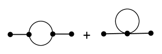
Figure 1: One-loop correction is sourced by cubic and quartic self-interactions of $\zeta$.

The one-loop corrected curvature power spectrum gives

$$\Bigl{[}\Delta^{2}_{\mathcal{R}}(k,t)\Bigr{]}_{\zeta{\rm loops}}\approx\frac{GH^{2}}{\pi\epsilon}\Bigl{\{}1+\frac{27GH^{2}}{4\pi\epsilon}\ln(a)+O(G^{2}H^{4})\Bigr{\}}\;.$$

This corresponds to a correction to the tree-level scalar mode function as

$$\Rightarrow u(t,k)\approx\frac{H}{\sqrt{2\epsilon}}\frac{1}{\sqrt{2k^{3}}}\Bigl{\{}1+\frac{27GH^{2}}{8\pi\epsilon}\,\ln(a)\Bigr{\}}\;,\qquad$$ (18)

if one uses Hartree approximation.

The $\zeta$-$\zeta$ correlator becomes time-dependent if there is least one undifferentiated field in the action at the relevant order. These so-called infrared logarithms, as well as $1/\epsilon$ term, enhance this one-loop effect by 3 orders of magnitude. But the smallness of $GH^{2}\approx 10^{-10}$ overshadows this enhancement and makes the total one-loop correction to be at most at the order of $10^{-6}$. The degree of the precision of the current experiments is well below the necessary level to untangle this one-loop effect. But still the effect is not hopelessly small.

For the last five years there has been some discussion about the time-dependence of the $\zeta$-$\zeta$ correlator. It has even been claimed LSMZ4 that this quantity is constant at all loops, which we find to be highly dubious since even at tree-level it only asymptotes to a constant. The point of this work is not to argue the time-dependence of $\zeta$-$\zeta$ correlator, but rather go towards another direction; which is loop corrections to three-point function and to see what the consequences of time dependence of $\zeta$ are. We believe that the real enhancement of time-dependent $\zeta$-$\zeta$ correlator arises if one calculates three-point function for $\zeta$. It turns out the one-loop correction to this quantity might totally dominate the tree-level result. Therefore when searching for enhanced quantum gravity corrections, the more interesting quantity to calculate is the three-point function, which is the subject of the next section.

III Bispectrum at tree-level

One can write the primordial bispectrum in terms of the Fourier transformed three-point function as

$$\langle\zeta_{\mathbb{k_{1}}}\zeta_{\mathbb{k_{2}}}\zeta_{\mathbb{k_{3}}}\rangle=(2\pi)^{3}\delta^{3}(\mathbb{k_{1}}+\mathbb{k_{2}}+\mathbb{k_{3}})B_{\zeta}(k_{1},k_{2},k_{3})\;.$$ (19)

Assuming a local form for the bispectrum where the non-Gaussian $\zeta$ field is produced from the Gaussian background $\zeta_{g}$ field as

$$\zeta(\mathbf{x}) = \zeta_{g}(\mathbf{x})+(3/5)f_{\text{NL}}\zeta_{g}^{2}(\mathbf{x})+\mathcal{O}(\zeta_{g}^{3})\;.$$ (20)

One can show that the bispectrum peaks at the so called “squeezed” triangle, for which one takes one wave number much smaller than the other two, i.e. $k_{1}\approx k_{2}\gg k_{3}$. For the case of squeezed limit bispectrum can be expressed in terms of power spectrum with the following equation

$$B_{\zeta}^{\rm{local}}(k_{1},k_{2},k_{3})_{k_{1}\approx k_{2}\gg k_{3}}\approx\frac{12}{5}f_{\text{NL}}P(k_{1})P(k_{3})\;,$$ (21)

where the late time limit of the power spectrum is

$$P(k) = |u_{k}|^{2}_{\eta\rightarrow 0}\;=\;\frac{H^{2}}{2\epsilon}\;\frac{1}{2k^{3}}\;.$$ (22)

If Creminelli-Zaldarriaga consistency cz condition for single field inflation models hold, the bispectrum in the local limit (or squeezed-limit) can be written as

$$B_{\zeta}(k_{3}\ll k_{1})\;=\;(1-n_{s})P(k_{1})P(k_{3})\;,$$ (23)

where $n_{s}(k)$ is called the spectral tilt index and is defined as

$$n_{s}-1\equiv\frac{dln(P(k))}{dln(k)}\;.$$ (24)

Instead of expressing the three-point function in terms of two-point functions, one can directly compute the in-in expectation value of $\zeta$ and use (8) for the interaction Hamiltonian and can get the following expression for the bispectrum ganc :

$$B_{\zeta}(k_{1},k_{2},k_{3}) = 8i\frac{\epsilon^{2}}{H^{2}}\sum_{k_{i}}(\frac{1}{k_{i}^{2}})u_{k_{1}}(\bar{\eta})u_{k_{2}}(\bar{\eta})u_{k_{3}}(\bar{\eta})$$ (25)

$$\times\int_{\eta_{0}}^{\bar{\eta}}d\eta\frac{1}{\eta^{3}}u_{k_{1}}^{{}^{\prime}*}u_{k_{2}}^{{}^{\prime}*}u_{k_{3}}^{{}^{\prime}*}+c.c.\;.$$

The main point of this calculation is the integral that we have in the above expression for the bispectrum,

$$\int_{\eta_{0}}^{\bar{\eta}}d\eta\frac{1}{\eta^{3}}\tilde{u}_{k_{1}}^{{}^{\prime}*}\tilde{u}_{k_{2}}^{{}^{\prime}*}\tilde{u}_{k_{3}}^{{}^{\prime}*}\;.$$ (26)

If we take the tree-order mode function for the above expression it is obvious that we will get a small non-Gaussianity. This is due to the fact that the three-point function, therefore non-Gaussianity, is proportional to the change of the mode function for each wave number $k_{1},k_{2},k_{3}$. Since for each mode the mode function itself goes to a constant after the horizon crossing, the change of those tree-level mode functions will be very small. On the other hand, the two-point function, therefore power spectrum, is proportional to the magnitude of the mode function. Let us highlight this point by giving equations:

$${\rm power\;spectrum} \sim \langle\zeta_{\mathbb{k_{1}}}\zeta_{\mathbb{k_{2}}}\rangle\sim\delta^{3}(\mathbb{k_{1}}+\mathbb{k_{2}})|u_{k}|^{2}$$

$${\rm non-Gaussianity} \sim \langle\zeta_{\mathbb{k_{1}}}\zeta_{\mathbb{k_{2}}}\zeta_{\mathbb{k_{3}}}\rangle$$ (27)

$$\sim \delta^{3}(\mathbb{k_{1}}+\mathbb{k_{2}}+\mathbb{k_{3}}){u}_{k_{1}}(\bar{\eta}){u}_{k_{2}}(\bar{\eta}){u}_{k_{3}}(\bar{\eta})$$

$$\times \int_{\eta_{0}}^{\bar{\eta}}d\eta\frac{1}{\eta^{3}}{u}_{k_{1}}^{{}^{\prime}*}{u}_{k_{2}}^{{}^{\prime}*}{u}_{k_{3}}^{{}^{\prime}*}+c.c.$$

IV One-loop correction to bispectrum: a particular example

We would like to find the answer to the following question: How big is the effect of loops to n-point functions of primordial curvature perturbation during Inflation? The answer of the above question for two-point and three-point functions is are related to the magnitude and the time derivative of the scalar mode functions, respectively.

One should do the full computation to give a definitive answer of time dependence of bispectrum. In this work, our aim is to show that it is possible to get huge enhancements at one-loop order and for that we would like to consider the simplest case where the external legs are corrected

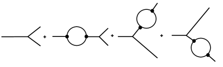
Figure 2: Bispectrum: Tree-level and corrections to external legs.

Here we would like to make a further simplification, namely use the form of the one-loop corrected mode function (III) where we applied a Hartree approximation.

The one-loop corrected mode function expression and its derivative with respect to conformal time and their long wavelength limits ($k\eta\ll 1$) are

$$u_{tree} = \frac{H}{\sqrt{2\epsilon}}\frac{1}{\sqrt{2k^{3}}}(1+ik\eta)e^{-ik\eta}$$ (28)

$$\Rightarrow \frac{H}{\sqrt{2}}\frac{1}{\sqrt{2k^{3}}}\Biggl{\{}1\;+\frac{k^{2}\eta^{2}}{2}+...\Biggr{\}}\;,$$

$${u}_{\rm 1-loop} \Rightarrow \frac{H}{\sqrt{2\epsilon}}\frac{1}{\sqrt{2k^{3}}}\Bigl{\{}1+O(1)GH^{2}\ln(a)\Bigr{\}}$$ (29)

$$= u_{tree}\Bigl{\{}1+O(1)\,\,GH^{2}\,\ln(a)\Bigr{\}}\;,$$

$$u_{tree}^{{}^{\prime}} \Rightarrow \frac{H}{\sqrt{2\epsilon}}\frac{1}{\sqrt{2k^{3}}}\Biggl{\{}k^{2}\eta+...\Biggr{\}}\;,$$ (30)

$${u}_{\rm 1-loop}^{{}^{\prime}} \Rightarrow \frac{H}{\sqrt{2\epsilon}}\frac{1}{\sqrt{2k^{3}}}k^{2}\eta\Bigl{\{}1+O(1)GH^{2}\frac{1}{k^{2}\eta^{2}}\Bigr{\}}$$ (31)

$$= u_{tree}^{{}^{\prime}}\Bigl{\{}1+O(1)GH^{2}\frac{1}{k^{2}\eta^{2}}+...\Bigr{\}}\;.$$

The difference between the one-loop corrected mode function’s and tree-level mode function’s time derivative is of the order of $GH^{2}$ $\approx 10^{-10}$ as expected, but also multiplied with an additional factor of $1/k^{2}\eta^{2}$. For the super-horizon modes ($k\eta\ll 1$) with the relevant 50 $e$-folds this brings an extra factor of $10^{20}$ which makes the one-loop correction to dwarf the tree-level part of the mode function.

The mathematical reasons for this huge effect is the following. The derivative with respect to conformal time brings an extra factor of $Ha(t)$ when it acts on a power of $a(t)$. Since the tree-level mode function is constant after horizon crossing, this time derivative does no good to boost the leading term, it simply annuls it. But for the case one-loop corrected mode function, the time derivative acts on the $\ln a$ and gives a chance to the constant leading term of the tree-level part of the mode function to survive. Not only does it survive, but also it gets boosted by the extra factor of $Ha(t)$.

Since the integral that appear in the the non-Gaussianity ($\zeta\zeta\zeta$ correlator) (III) has three factors of ${u}_{\rm 1-loop}^{{}^{\prime}}$ the one-loop correction to the three-point function is 30 orders magnitude bigger than the tree-level term. Since the one-loop correction to $P(k)$ terms are very small, this extremely large value of bispectrum can only be achieved by having a huge $f_{\rm NL}$ parameter, if we look at equation (21). It also implies that Creminelli-Zaldarriaga consistency condition for single scalar field is not satisfied here, since equation (23) could not be satisfied with a bispectrum this big. However this does not mean the invalidation of the consistency condition, since the condition assumes time-independency a priori, although there are cases where the condition is violated rms ; nfs . But most importantly an $f_{\rm NL}$ parameter of this magnitude results into ruling out all single field inflation models due to the observational limits on the non-Gaussianity parameter.

We would like to point out that we are not claiming Weinberg’s theorem is incorrect. Mathematically what happens is that, the time derivative acting on the constant term, which is the leading term in the long wavelength expansion of scalar mode function kills it. On the other hand, the quantum corrected time-dependent mode functions long wavelength expansion leave a room for the constant term to survive by letting the time derivative hit on the infrared logarithm. Due to this wondrous interaction, these one-loop terms dominate the tree-level term by 30 orders of magnitude, which results in breaking down of the perturbation theory. Therefore as Weinberg pointed out SW2 we see the need of a non-perturbative method for cosmological correlations.

The integrals that appear in (III) can be evaluated BK analytically in a general vacuum choice, called non-Bunch-Davies initial state which would lead to an increase of the non-Gaussianity parameter $f_{\rm NL}$ even at the tree-level ganc ; ap . For the case of non-Bunch-Davies initial state the one-loop term again dominates the tree-level one and be ruled out as well.

V Discussion

The success of inflationary cosmology is appalling. This simple idea solves homogeneity, flatness, horizon, isotropy and primordial monopole problems of standard cosmology with a single shot guth ; linde ; bst . With inflation, linking quantum physics with cosmology, we can understand the origin of all matter from primordial quantum fluctuations. Getting first quantum gravitational data, such as curvature power spectrum with small error bars is a major success in itself.

It is therefore time to go beyond this tree-level effect and investigate possible consequences, which we can name as precision inflationary cosmology. Towards this direction, one possible thing to do is calculating loop corrections to cosmological correlations. At first look, one would naturally think that this is a futile effort due to the smallness of the loop counting parameter $GH^{2}$. But still there was a lot of attention to loop corrections to power spectrum despite the smallness of them.

Cosmological loop corrections bring a typical infrared logarithm and are divided into three categories according to the form of the logarithmic factors: $Log(H\mu)$, $Log(kL)$ and $Log(a(t))$ LSMZ3 . The first case is claimed to be due to making an error in the implementing diffeomorphism invariant regularization and the second being a projection effect that will be removed if one computes observable quantities. The final case is also dismissed in the mentioned work on the grounds of symmetry arguments as well as extrapolating this time-dependent effect to reheating and baryogenesis and claiming that predictivity of inflation will be lost. One can certainly reply to the above criticisms and perhaps one should. But in this work, we would like to bring a different viewpoint to this discussion that is more dramatic.

First of all, time-dependent zeta do occur even without loop corrections, such as multifield inflationary models and entropy perturbations. The time-dependence that we are interested in, that has the form of $Log(a(t))$, are originated from loop corrections. We investigated the minimal case where the only scalar field is the inflaton. We first reviewed time-dependent loop corrections to two-point functions, i.e. power spectrum, which arises due to $\zeta$-$\zeta$ self interactions at one-loop order. In principle they are important; on the other hand, from an observational perspective they are irrelevant at the moment. We took the one-loop corrected scalar mode function and used that to calculate the loop corrections to external legs of the three-point function using Hartree approximation. We concluded that they grow with the square of the scale factor. We showed that the loop corrections have the potential of dominating the tree-level term by 30 orders of magnitude and lead to breaking down of the perturbation theory. If this effect survives after a nonperturbative analysis, that would result into an immediate ruling out all single-scalar driven models of inflation.

Therefore, non-Gaussianity is a better place, compared to power spectrum, to look for quantum gravitational corrections. The technical reason of this is:

1. Power spectrum is related to the magnitude of mode function.
   Therefore it goes like : constant (tree-level) + a small correction (loops)

2. Non-Gaussianity is related to the time derivative of the mode function.
   Therefore it goes like : almost zero (tree-level) + a not so small correction(loops) compared to zero

Therefore the real treasure is hidden in the higher order correlation functions, not in the power spectrum. We also showed that this would imply a huge ($10^{20}$ times bigger than tree-level prediction) non-Gaussianity $f_{\rm NL}$ parameter, leading to an immediate contradiction with the constraints on observed value of $f_{\rm NL}$ parameter.

At this point we would like to discuss the possible ways of avoiding huge $f_{\rm NL}$ parameter. Let us remember that there is another type of diagram that will contribute at one-loop order to three-point function. It might turn out that this vertex correction (Fig. 3) cancel the total contribution coming from Fig. 2.

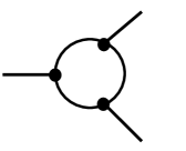
Figure 3: The remaining diagram at one-loop order.

For that end it is useful to look at the work of Cogolo et al. crv , where they show that this kind of diagram dominates the whole series of diagrams. They consider and extra scalar field and the effect arises due to that; but still a similar thing might happen for the single scalar field situation.

We want to conclude the discussion section by giving six points that should further be investigated in detail which might change the picture:

1. Vertex correction

2. Hartree approximation

3. Single scalar field (inflaton), adiabatic perturbations

4. Time-dependent $\zeta$-$\zeta$ correlator from loops

5. Almost constant slow-roll parameter $\epsilon$

6. A nonperturbative analysis.

The first possibility is the vertex correction exactly cancelling the effects given above. It might be that using Hartree approximation is the source of the mentioned effect. For that, one should do the full calculation and see if the effect is not there. One can imagine scenarios where a spectator field causing a similar effect which might cancel the $\zeta$ loops. This only happens for particular situations crv . One could also try to incorporate the time-dependence of the $\epsilon$ parameter and investigate the consequences of that.

Our work highlights the need of a nonperturbative method to cosmological correlations. A nonperturbative method was found by Starobinsky and Yokoyoma sy for self-interacting scalar fields and Tsamis and Woodard for Scalar Quantum Electrodynamics tw , where they were able to resum the leading infrared log terms in the whole perturbative series. And it might turn out that, one can avoid a big $f_{\rm NL}$ parameter after calculating the quantum effects using a nonperturbative method. One can simply say that it is the fourth assumption that is wrong and maybe it is so. But no matter what the solution is, quantum loop corrections that result into time-dependent scalar mode functions have consequences that are so important and will be of such magnitude that they can not be swept under the rug.

We would like to end our discussion by pointing out to a curious work done by Pattison et al. PVAW , where the probability density function (PDF) of curvature perturbations were calculated by using stochastic $\delta N$ formalism. During this period, due to quantum diffusion effects, stochastic force would determine the inflaton dynamics and PDF of $\zeta$ has the form elliptic theta functions. They claim that, in the limit where the potential is exactly flat and stochastic effects dominate, one gets highly non-Gaussian curvature perturbations. This claim, which might be an artefact of using stochastic $\delta N$ formalism, should certainly be checked by making rigorous loop calculations. This work also shows the need for doing a one-loop calculation (fully renormalized with all the relevant interactions included) of the three-point function in particular and n-point functions of $\zeta$ in general.

References

- (1) V. F. Mukhanov and G. V. Chibisov,Pisma Zh. Eksp. Teor. Fiz. 33, 549 (1981) [JETP Lett. 33, 532 (1981)].
- (2) A. A. Starobinsky, Pisma Zh. Eksp. Teor. Fiz. 30, 719 (1979). [JETP Lett. 30, 682 (1979)].
- (3) S. Weinberg, Phys. Rev. D 72, (2005) 043514.
- (4) S. Weinberg, Phys. Rev. D 74, (2006) 023508.
- (5) L. Senatore and M. Zaldarriaga, Zaldarriaga, J. High Energy Phys. 12 (2010) 008.
- (6) E. O. Kahya, V. K. Onemli and R. P. Woodard, Phys. Lett. B 694 101 (2010).
- (7) L. Senatore and M. Zaldarriaga, J. High Energy Phys. 01 (2013) 109.
- (8) G. L. Pimentel, L. Senatore and M. Zaldarriaga, J. High Energy Phys. 07 (2012) 166.
- (9) L. Senatore and M. Zaldarriaga, J. High Energy Phys. 09 (2013) 148.
- (10) S. B. Giddings, M. S. Sloth, Sloth, J. Cosmol. Astropart. Phys. 01 (2011) 023.
- (11) H. R. S. Cogollo, Y. Rodriguez and C. A. Valenzuela-Toledo, J. Cosmol. Astropart. Phys. 08, (2008) 029.
- (12) P.A.R. Ade et al. (Planck Collaboration), Astron. Astrophys. 594, A17 (2016).
- (13) J. Maldacena, J. High Energy Phys. 05 (2003) 013.
- (14) T. S. Bunch and P. Davies, Proc. R. Soc. A 360, 117 (1978).
- (15) A. R. Liddle and D. H. Lyth, Cosmological inflation and large scale structure (Cambridge University Press, 2000).
- (16) P.A.R. Ade et al. (Planck Collaboration), Astron. Astrophys. 594, A13 (2016).
- (17) T. Tanaka and Y. Urakawa, J. Cosmol. Astropart. Phys. 06 (2016) 020.
- (18) N. Katirci, A. Kaya and M. Tarman, J. Cosmol. Astropart. Phys. 06 (2014) 022.
- (19) T. Tanaka and Y. Urakawa, Urakawa, Classical Quantum Gravity 30, 233001 (2013).
- (20) S. B. Giddings and M. S. Sloth, Phys. Rev. D 84, 063528 (2011).
- (21) S. B. Giddings and M. S. Sloth, J. Cosmol. Astropart. Phys. 01 (2011) 023.
- (22) E.O. Kahya, V.K. Onemli and R.P. Woodard, Phys. Rev. D 81, 023508 (2010).
- (23) P. Adshead, R. Easther and E. A. Lim, Phys. Rev. D 79 063504 (2009) .
- (24) D. Seery, J. Cosmol. Astropart. Phys. 02 (2008) 006.
- (25) D. Boyanovsky, H. J. de Vega and N. G. Sanchez, Nucl. Phys. B 747 25 (2006).
- (26) Y. Wu and J. Yokoyama, arXiv:1704.05026.
- (27) N. Bartolo, E. Dimastrogiovanni and A. Vallinotto, J. Cosmol. Astropart. Phys. 11, (2010) 003.
- (28) E. Dimastrogiovanni and N. Bartolo, J. Cosmol. Astropart. Phys. 11, (2008) 016.
- (29) P. Creminelli and M. Zaldariga, J. Cosmol. Astropart. Phys. 10, (2004) 006.
- (30) J. Ganc, Phys. Rev. D 84, 063514 (2011).
- (31) A. E. Romano, S. Mooij and M. Sasaki, Phys. Lett. B 761, 119 (2016).
- (32) M. H. Namjoo, H. Firouzjahi and M. Sasaki Europhys. Lett. 101, 39001 (2013).
- (33) S. Boran and E. O. Kahya (unpublished).
- (34) I. Agullo and L. Parker, Phys. Rev. D 83, 063526 (2011).
- (35) A. Guth, Phys. Rev. D 23, 347 (1981).
- (36) A. D. Linde, Phys. Lett. B 108, 389 (1982).
- (37) J. M. Bardeen, P. J. Steinhardt and M. S. Turner, Phys. Rev. D 28, 679 (1983).
- (38) A. A. Starobinsky and J. Yokoyoma, Phys. Rev. D 50, 6357 (1994).
- (39) T. Prokopec, N. C. Tsamis and R. P. Woodard, Classical Quantum Gravity 24, 201 (2007).
- (40) C. Pattison, V. Vennin, H. Assadullahi and D. Wands, J. Cosmol. Astropart. Phys. 10, (2017) 046.