Exact Solutions of Space-time Fractional EW and modified EW equations

Abstract

The bright soliton solutions and singular solutions are constructed for space-time fractional EW and modified EW equations. Both equations are reduced to ordinary differential equations by the use of fractional complex transform and properties of modified Riemann-Liouville derivative. Then, implementation of ansatz method the solutions are constructed.
Keywords: Fractional EW equation, Fractional MEW equation, bright soliton, singular solution.

1 Introduction

Several decades ago, more generalized forms of differential equations are described as fractional differential equations. Various phenomena in many natural and social sciences fields like engineering, geology, economics, meteorology, chemistry and physics are modeled by those equations[1, 2]. The descriptions of diffusion, diffusive convection, Fokker-Plank type, evolution, and other differential equations are expanded by using fractional derivatives. Some well known fractional partial differential equations (FPDE) in literature can be listed as diffusion equation, nonlinear Schrödinger equation, Ginzburg-Landau equation, Landau-Lifshitz, Boussinesq equations, etc.[2].

Even though there exist general methods for solutions of linear partial differential equations, the class of nonlinear partial differential equations have usually exact solutions. Sometimes it is also possible to obtain soliton-type solitary wave solutions, which behaves like particles, that is, maintains its shape with constant speed and preserves its shape after collision with another soliton, for partial differential equations. The famous nonlinear partial differential equations having soliton solutions in literature are KdV, and Schrödinger equations. Soliton type solutions have great importance in optics, fluid dynamics, propagation of surface waves, and many other fields of physics and various engineering branches.

The integer ordered form

$$U_{t}(x,t)-U(x,t)U_{x}(x,t)-U_{xxt}(x,t)=0$$ (1)

was named as the Equal-width Equation (EWE) by Morrison et al.[3] due to having traveling wave solutions containing $\operatorname{sech}^{2}{}$ function. The EWE has only lowest three polynomial conservation laws and they were determined in the same study. The single traveling wave solutions to the generalized form of the EWE are classified by implementing the complete discrimination system for polynomial[4]. Owing to having analytical solutions, the EWE also attracts many researchers studying numerical techniques for partial differential equations. So far, various numerical methods covering differential quadrature, Galerkin and meshless methods[5], lumped Galerkin methods based on B-splines[6, 7], septic B-spline collocation[8], the method of lines based on meshless kernel [9] have been applied to solve the EWE numerically.

Recently, parallel to developments in symbolic computations, lots of new techniques have been proposed to solve nonlinear partial differential equations exactly. Some of those methods covering the first integral method, the sub-equation method, Kudryashov method, and ansatz methods have been applied for exact solutions for not only integer ordered and but also fractional ordered partial differential equations[10, 11, 12, 13, 14]. Some recent studies including various methods for exact solutions of fractional partial differential equations in literature can be found in[15, 16, 17, 18, 19, 20, 21, 22].

This study aims to generate exact solutions for the space-time fractional equal-width equation (FEWE) and modified fractional equal-width equation (MFEWE) of the forms

$$D_{t}^{\alpha}u(x,t)+\epsilon D_{x}^{\alpha}u^{2}(x,t)-\delta D_{xxt}^{3\alpha}u(x,t)=0$$ (2)

and

$$D_{t}^{\alpha}u(x,t)+\epsilon D_{x}^{\alpha}u^{3}(x,t)-\delta D_{xxt}^{3\alpha}u(x,t)=0$$ (3)

where $\epsilon$ and $\delta$ are real parameters and the modified Riemann-Liouville derivative (MRLD) operator of order $\alpha$ for the continuous function $u:\mathbb{R}\rightarrow\mathbb{R}$ defined as

$$D_{x}^{\gamma}u(x)=\left\{\begin{array}[]{lcc}\dfrac{1}{\Gamma{(-\gamma)}}\int\limits_{0}^{x}(x-\eta)^{-\gamma-1}u(\eta)d\eta,\quad\gamma<0\\ \dfrac{1}{\Gamma{(-\gamma)}}\dfrac{d}{dx}\int\limits_{0}^{x}(x-\eta)^{-\gamma}[u(\eta)-u(0)]d\eta,\quad 0<\gamma<1\\ (u^{(p)(x)})^{(\gamma-p)},\quad p\leq\gamma\leq p+1,\quad p\geq 1\end{array}\right.$$ (4)

where the Gamma function is given as

$$\Gamma(\gamma)=\lim\limits_{p\rightarrow\infty}\dfrac{p!p^{\gamma}}{\gamma(\gamma+1)(\gamma+2)\ldots(\gamma+p)}$$ (5)

[23].

2 The properties of the MRLD and Methodology of Solution

Some properties of the MRLD can be listed as

$$D_{x}^{\alpha}x^{c} =\dfrac{\Gamma{(1+c)}}{\Gamma{(1+c-\alpha)}}$$ (6)

$$D_{x}^{\alpha}\{aw(x)+bv(x)\} =aD_{x}^{\alpha}\{w(x)\}+bD_{x}^{\alpha}\{v(x)\}$$

where $a,b$ are constants and $c\in\mathbb{R}$ [24].

Consider the nonlinear FPDEs of the general implicit polynomial form

$$F(u,D_{t}^{\alpha}u,D_{x}^{\theta}u,D_{t}^{\alpha}D_{t}^{\alpha}u,D_{t}^{\alpha}D_{t}^{\alpha}u,D_{t}^{\alpha}D_{x}^{\theta}u,D_{x}^{\theta}D_{x}^{\theta}u,\ldots)=0,\quad 0<\alpha,\theta<1$$ (7)

where $\alpha$ and $\theta$ are orders of the MRLD of the function $u=u(x,t)$. The fractional complex transform

$$u(x,t)=U(\xi),\quad\xi=\dfrac{\tilde{k}x^{\theta}}{\Gamma{(1+\theta)}}-\dfrac{\tilde{c}t^{\alpha}}{\Gamma{(1+\alpha)}}$$ (8)

where $\tilde{k}$ and $\tilde{c}$ are nonzero constants reduces (7) to an integer order differential equation [25]. One should note that the chain rule can be calculated as

$$D_{t}^{\alpha}u =\sigma_{1}\dfrac{dU}{d\xi}D_{t}^{\alpha}\xi$$ (9)

$$D_{x}^{\alpha}u =\sigma_{2}\dfrac{dU}{d\xi}D_{x}^{\alpha}\xi$$

where $\sigma_{1}$ and $\sigma_{2}$ fractional indices[26]. Substitution of fractional complex transform (8) into (7) and usage of chain rule defined (9) converts (7) to an ordinary differential equation of the polynomial form

$$G(U,\frac{dU}{d\xi},\frac{d^{2}U}{d\xi^{2}},\ldots)=0$$ (10)

3 Solutions for fractional EW equation

Consider the FEWE equation

$$D_{t}^{\alpha}u(x,t)+\epsilon D_{x}^{\alpha}u^{2}(x,t)-\delta D_{xxt}^{3\alpha}u(x,t)=0$$ (11)

$$t>0,\quad 0<\alpha\leq 1$$

The use of the transformation (8) reduces the FEWE (11) to

$$-cU^{\prime}+\epsilon k(U^{2})^{\prime}+\delta ck^{2}U^{\prime\prime\prime}=0$$ (12)

where $k=\tilde{k}\sigma_{2}$ and $c=\tilde{c}\sigma_{1}$

3.1 Bright soliton solution

Let $A$, $\tilde{k}$ and $\tilde{c}$ be arbitrary constants. Then, assume that

$$U(\xi)=A\operatorname{sech}^{p}{\xi},\quad\xi=\dfrac{\tilde{k}x^{\alpha}}{\Gamma{(1+\alpha)}}-\dfrac{\tilde{c}t^{\alpha}}{\Gamma{(1+\alpha)}}$$ (13)

solves Eq. (12). Substituting the solution into the equation (12) leads to

$$(-\delta\,cp{k}^{2}A-\delta\,cp^{2}{k}^{2}A)\operatorname{sech}^{p+2}{\xi}+\epsilon kA^{2}\operatorname{sech}^{2p}{\xi}+(\delta ck^{2}p^{2}-cA)\operatorname{sech}^{p}{\xi}=0$$ (14)

Equating the powers $p+2=2p$ gives $p=2$. Substituting $p=2$ into Eq.(14) reduces it to

$$\left(-6\,\delta\,c{k}^{2}A+\epsilon\,k{A}^{2}\right)\operatorname{sech}^{4}\xi+\left(4\,\delta\,c{k}^{2}A-cA\right)\operatorname{sech}^{2}\xi=0$$ (15)

and solving Eq.(15) for nonzero $\operatorname{sech}^{4}{\xi}$ and $\operatorname{sech}^{2}{\xi}$ gives

$$A =\mp 3c\frac{\sqrt{\delta}}{\epsilon}$$ (16)

$$k =\mp\frac{1}{2}\sqrt{\frac{1}{\delta}}$$

Thus the bright soliton solution is formed as

$$u(x,t)=A\operatorname{sech}^{2}\left(\dfrac{\tilde{k}x^{\alpha}}{\Gamma{(1+\alpha)}}-\frac{\tilde{c}t^{\alpha}}{\Gamma{(1+\alpha)}}\right)$$ (17)

where $A$ is given in (16). The simulations of motion of bright solitons for various values of $\alpha$ are demonstrated in Fig(1(a)-1(d)) for $\delta=1$, $\epsilon=3$ and $c=1$.

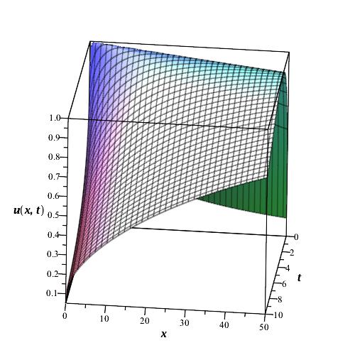
(a) $\alpha=0.25$

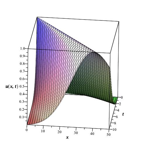
(b) $\alpha=0.50$

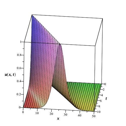
(c) $\alpha=0.75$

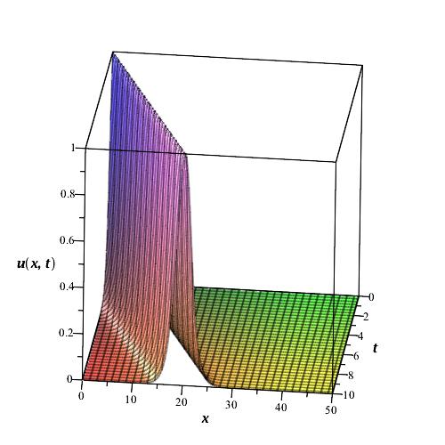
(d) $\alpha=1.00$

Figure 1: Bright soliton solutions of FEWE for various values of $\alpha$

3.2 Singular Solution

Let

$$U(\xi)=A\operatorname{csch}^{p}{\xi},\quad\xi=\dfrac{\tilde{k}x^{\alpha}}{\Gamma{(1+\alpha)}}-\dfrac{\tilde{c}t^{\alpha}}{\Gamma{(1+\alpha)}}$$ (18)

be a solution for the equation (12) with $A$, $\tilde{k}$ and $\tilde{c}$ arbitrary constants. Since the solution has to satisfy the equation (12), substituting it into the equation gives

$$\left(\delta pc{k}^{2}A+\delta p^{2}c{k}^{2}A\right)\operatorname{csch}^{p+2}{\xi}+\left(\delta p^{2}c{k}^{2}A-Ac\right)\operatorname{csch}^{p}{\xi}+\epsilon kA^{2}\operatorname{csch}^{2p}{\xi}=0$$ (19)

Choosing $p+2=2p$ gives $p=2$ and reduces (19) to

$$\left(6\,\delta\,c{k}^{2}A+\epsilon\,k{A}^{2}\right)\operatorname{csch}^{4}{\xi}+\left(4\,\delta\,c{k}^{2}A-Ac\right)\operatorname{csch}^{2}{\xi}=0$$ (20)

Solution of (20) for nonzero $\operatorname{csch}$ function give

$$A =\pm\dfrac{3c\sqrt{\delta}}{\epsilon}$$ (21)

$$k =\pm\dfrac{1}{2}\sqrt{\dfrac{1}{\delta}}$$

Thus the singular solution of Eq.(12) becomes

$$U(\xi)=A\operatorname{csch}^{p}{\dfrac{\tilde{k}x^{\alpha}}{\Gamma{(1+\alpha)}}-\dfrac{\tilde{c}t^{\alpha}}{\Gamma{(1+\alpha)}}}$$ (22)

where $A$ and $k$ are given (21). The singular solution simulations for various $\alpha$ values and $\epsilon=3$, $\delta=c=1$ are plotted in Fig.(2(a)-2(d)).

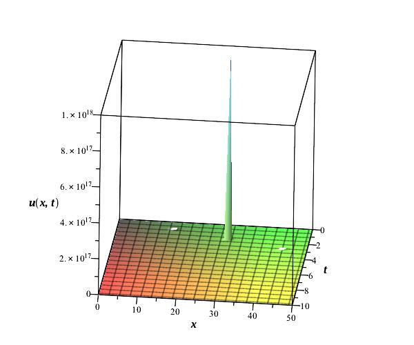
(a) $\alpha=0.25$

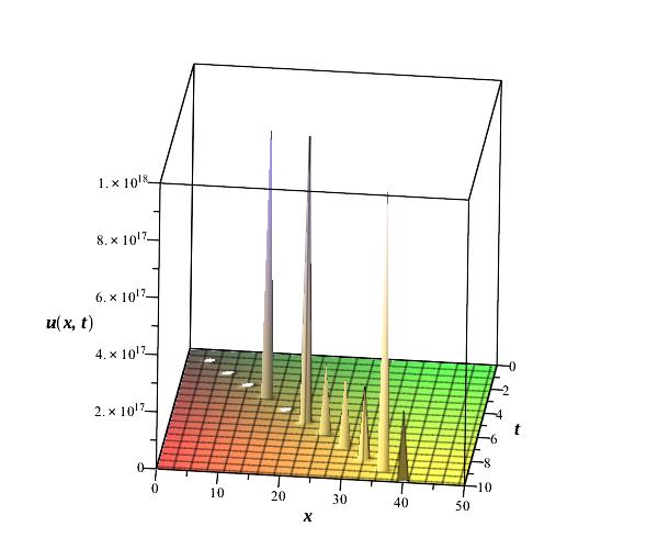
(b) $\alpha=0.50$

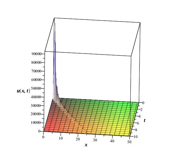
(c) $\alpha=0.75$

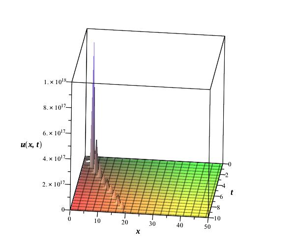
(d) $\alpha=1.00$

Figure 2: Singular solutions of FEWE for various values of $\alpha$

4 Solutions for fractional modified EW equation

Consider space-time fractional modified equally width equation of the form

$$D_{t}^{\alpha}u(x,t)+\epsilon D_{x}^{\alpha}u^{3}(x,t)-\delta D_{xxt}^{3\alpha}u(x,t)=0$$ (23)

The use of the transformation (8) converts the MFEWE (23) to

$$-cU^{\prime}+\epsilon k(U^{3})^{\prime}+\delta ck^{2}U^{\prime\prime\prime}=0$$ (24)

where $k=\tilde{k}\sigma_{2}$ and $c=\tilde{c}\sigma_{1}$.

4.1 Bright Soliton Solution

Assume that the FMEWE (23) has a solution of the form (13). Substitution of (13) into the FMEWE (23) generates the equation

$$\left(-\delta cAk^{2}p-\delta ck^{2}Ap^{2}\right)\operatorname{sech}^{p+2}{\xi}+\left(\delta cAk^{2}p^{2}-cA\right)\operatorname{sech}^{p}{\xi}+\epsilon kA^{3}\operatorname{sech}^{3p}{\xi}=0$$ (25)

Equating the powers $p+2=3p$ gives $p=1$. Substituting $p=1$ into (25) and rearrangement gives the equation

$$\left(\epsilon k{A}^{3}-2\delta c{k}^{2}A\right)\operatorname{sech}^{3}{\xi}+\left(\delta c{k}^{2}A-cA\right)\operatorname{sech}{\xi}=0$$ (26)

Solving the coefficients of (26) for $A$ and $k$ under the assumption $\operatorname{sech}{\xi}\neq 0$ gives

$$A =\pm\sqrt{2}\sqrt{\pm\frac{c\sqrt{\delta}}{\epsilon}}$$ (27)

$$k =\pm\frac{1}{\sqrt{\delta}}$$

Thus, the bright soliton solution for the FMEWE is constructed as

$$u(x,t)=A\operatorname{sech}\left(\dfrac{\tilde{k}x^{\alpha}}{\Gamma{(1+\alpha)}}-\frac{\tilde{c}t^{\alpha}}{\Gamma{(1+\alpha)}}\right)$$ (28)

where $A$ is given as above. The simulations of bright solitons are depicted for various $\alpha$ values in Fig(3(a)-3(d)).

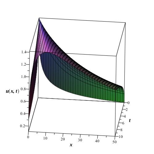
(a) $\alpha=0.25$

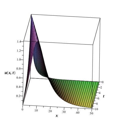
(b) $\alpha=0.50$

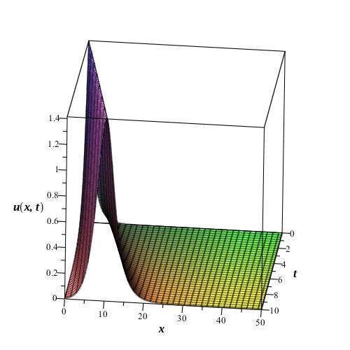
(c) $\alpha=0.75$

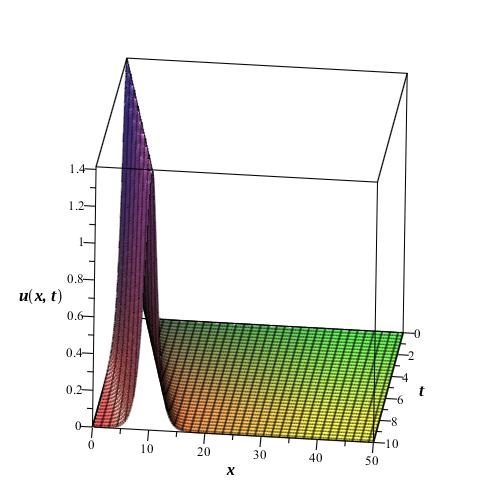
(d) $\alpha=1.00$

Figure 3: Bright soliton solutions of MFEWE for various values of $\alpha$

4.2 Singular Solution

Assume that

$$U(\xi)=A\operatorname{csch}^{p}{\xi},\quad\xi=\dfrac{\tilde{k}x^{\alpha}}{\Gamma{(1+\alpha)}}-\dfrac{\tilde{c}t^{\alpha}}{\Gamma{(1+\alpha)}}$$ (29)

is a solution for the equation (24) with $A$, $\tilde{k}$ and $\tilde{c}$ arbitrary constants. Substitution of the solution (29) into the equation (24) gives

$$\left(\delta ck^{2}Ap+\delta ck^{2}Ap^{2}\right)\operatorname{csch}^{p+2}{\xi}+\left(\delta ck^{2}Ap^{2}-cA\right)\operatorname{csch}^{p}{\xi}+\epsilon kA^{3}\operatorname{csch}^{3p}{\xi}=0$$ (30)

Choice of $p=1$ gives

$$\left(A^{3}\epsilon k+2Ac\delta k^{2}\right)\operatorname{csch}^{3}{\xi}+\left(Ac\delta k^{2}-Ac\right)\operatorname{csch}{\xi}=0$$ (31)

Solving the equation for nonzero $\operatorname{csch}{\xi}$ gives

$$A =\pm\sqrt{\pm 2\frac{c\sqrt{\delta}}{\epsilon}}$$ (32)

$$k =\pm\frac{1}{\sqrt{\delta}}$$

Thus, the singular solution of the FMEWE is formed as

$$u(x,t)=A\operatorname{csch}\left(\dfrac{\tilde{k}x^{\alpha}}{\Gamma{(1+\alpha)}}-\frac{\tilde{c}t^{\alpha}}{\Gamma{(1+\alpha)}}\right)$$ (33)

where $A$ and $k$ are given in Eq.(32). The singular solution simulations for various $\alpha$ values and $\epsilon=\delta=c=1$ with $k=1/\sqrt{\delta}$ and $A=\sqrt{2c\sqrt{\delta}/\epsilon}$ are plotted in Fig.(4(a)-4(d)).

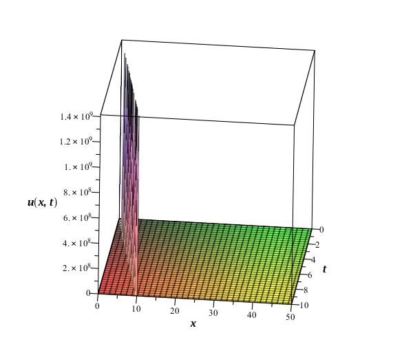
(a) $\alpha=0.25$

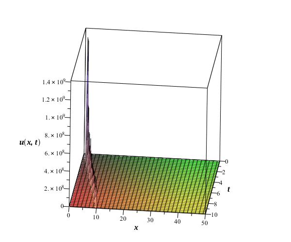
(b) $\alpha=0.50$

(c) $\alpha=0.75$

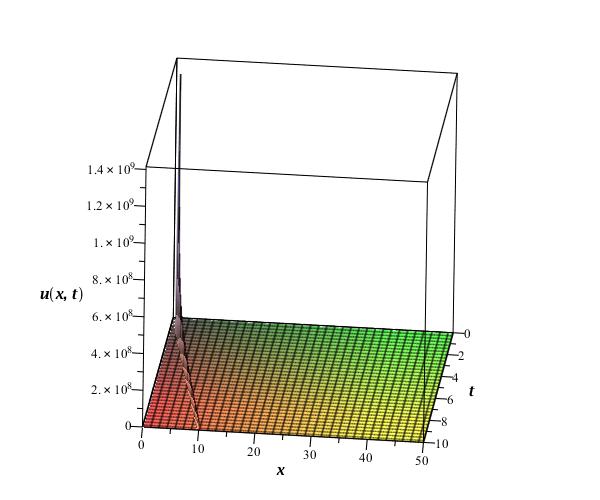
(d) $\alpha=1.00$

Figure 4: Singular solutions of FMEWE for various values of $\alpha$

5 Conclusion

In the study, the bright soliton solutions and singular solutions for space-time fractional EW equation and modified EW equation are obtained by ansatz method. After reducing both equations to integer-ordered ordinary differential equations, the $\operatorname{sech}$ and $\operatorname{csch}$ type solutions are investigated. Substituting ansatzs into the integer-ordered ordinary differential equations, the nonzero coefficients in solutions are determined. The graphs of all solutions are depicted for suitable coefficients.

References

- [1] Podlubny, I. (1998). Fractional differential equations: an introduction to fractional derivatives, fractional differential equations, to methods of their solution and some of their applications (Vol. 198). Academic press.
- [2] Guo, B. L., Pu, X. K., & Huang, F. H. (2011). Fractional Partial Differential Equations and Their Numerical Solutions. Science Press, Beijing, China.
- [3] Morrison, P. J., Meiss, J. D., & Cary, J. R. (1984). Scattering of regularized-long-wave solitary waves. Physica D: Nonlinear Phenomena, 11(3), 324-336.
- [4] Fan, H. L. (2012). The classification of the single traveling wave solutions to the generalized equal width equation. Applied Mathematics and Computation, 219(2), 748-754.
- [5] Saka, B., Dağ, İ., Dereli, Y., & Korkmaz, A. (2008). Three different methods for numerical solution of the EW equation. Engineering analysis with boundary elements, 32(7), 556-566.
- [6] Esen, A. (2005). A numerical solution of the equal width wave equation by a lumped Galerkin method. Applied mathematics and computation, 168(1), 270-282.
- [7] Karakoç, S. B. G., & Geyikli, T. (2012). Numerical solution of the modified equal width wave equation. International Journal of Differential Equations, 2012.
- [8] Geyikli, T., & Karakoc, S. B. G. (2011). Septic B-spline collocation method for the numerical solution of the modified equal width wave equation. Applied Mathematics, 2(06), 739.
- [9] Dereli, Y., & Schaback, R. (2013). The meshless kernel-based method of lines for solving the equal width equation. Applied Mathematics and Computation, 219(10), 5224-5232.
- [10] Güner, Ö., Bekir, A., & Karaca, F. (2016). Optical soliton solutions of nonlinear evolution equations using ansatz method. Optik-International Journal for Light and Electron Optics, 127(1), 131-134.
- [11] Bekir, A., & Güner, Ö. (2013). Bright and dark soliton solutions of the (3+1)-dimensional generalized Kadomtsev-Petviashvili equation and generalized Benjamin equation. Pramana, 81(2), 203-214.
- [12] Ebadi, G., Mojaver, A., Triki, H., Yildirim, A., & Biswas, A. (2013). Topological solitons and other solutions of the Rosenau-KdV equation with power law nonlinearity. Romanian Journal of Physics, 58(1-2), 1-10.
- [13] Biswas, A., Kumar, S., Krishnan, E. V., Ahmed, B., Strong, A., Johnson, S., & Yildirim, A. (2013). Topological solitons and other solutions to potential Korteweg-de Vries equation. Romanian Reports in Physics, 65(4), 1125-1137.
- [14] Biswas, A., Ebadi, G., Triki, H., Yildirim, A., & Yousefzadeh, N. (2013). Topological soliton and other exact solutions to KdV-Caudrey-Dodd-Gibbon equation. Results in Mathematics, 63(1-2), 687-703.
- [15] Bekir, A., & Güner, Ö. (2013). Exact solutions of nonlinear fractional differential equations by (G?/G)-expansion method. Chinese Physics B, 22(11), 110202.
- [16] Güner, Ö., & Cevikel, A. C. (2014). A procedure to construct exact solutions of nonlinear fractional differential equations. The Scientific World Journal, 2014.
- [17] Bekir, A., Güner, Ö., & Ünsal, Ö. (2015). The first integral method for exact solutions of nonlinear fractional differential equations. Journal of Computational and Nonlinear Dynamics, 10(2), 021020.
- [18] Bekir, A., & Guner, O. (2014). Exact solutions of distinct physical structures to the fractional potential Kadomtsev-Petviashvili equation. Computational Methods for Differential Equations, 2(1), 26-36.
- [19] Bekir, A., & Güner, Ö. (2014). Analytical Approach for the Space-time Nonlinear Partial Differential Fractional Equation. International Journal of Nonlinear Sciences and Numerical Simulation, 15(7-8), 463-470.
- [20] Bekir, A., & Güner, Ö. (2014). The-expansion method using modified Riemann-Liouville derivative for some space-time fractional differential equations. Ain Shams Engineering Journal, 5(3), 959-965.
- [21] Mirzazadeh, M., Eslami, M., & Biswas, A. (2014). Solitons and periodic solutions to a couple of fractional nonlinear evolution equations. Pramana, 82(3), 465-476.
- [22] Taghizadeh, N., Mirzazadeh, M., Rahimian, M., & Akbari, M. (2013). Application of the simplest equation method to some time-fractional partial differential equations. Ain Shams Engineering Journal, 4(4), 897-902.
- [23] Jumarie, G. (2009). Table of some basic fractional calculus formulae derived from a modified Riemann-Liouville derivative for non-differentiable functions. Applied Mathematics Letters, 22(3), 378-385.
- [24] Annaby, M. H., & Mansour, Z. S. (2012). Q-fractional Calculus and Equations (Vol. 2056). Springer.
- [25] Li, Z. B., & He, J. H. (2010). Fractional complex transform for fractional differential equations. Math. Comput. Appl, 15(5), 970-973.
- [26] He, J. H., Elagan, S. K., & Li, Z. B. (2012). Geometrical explanation of the fractional complex transform and derivative chain rule for fractional calculus. Physics Letters A, 376(4), 257-259.