Visibility Graphs, Dismantlability, and the Cops and Robbers Game

Abstract

We study versions of cop and robber pursuit-evasion games on the visibility graphs of polygons, and inside polygons with straight and curved sides. Each player has full information about the other player’s location, players take turns, and the robber is captured when the cop arrives at the same point as the robber. In visibility graphs we show the cop can always win because visibility graphs are dismantlable, which is interesting as one of the few results relating visibility graphs to other known graph classes. We extend this to show that the cop wins games in which players move along straight line segments inside any polygon and, more generally, inside any simply connected planar region with a reasonable boundary. Essentially, our problem is a type of pursuit-evasion using the link metric rather than the Euclidean metric, and our result provides an interesting class of infinite cop-win graphs.

1 Introduction

Pursuit-evasion games have a rich history both for their mathematical interest and because of applications in surveillance, search-and-rescue, and mobile robotics. In pursuit-evasion games one player, called the “evader,” tries to avoid capture by “pursuers” as all players move in some domain. There are many game versions, depending on whether the domain is discrete or continuous, what information the players have, and how the players move—taking turns, moving with bounded speed, etc.

This paper is about the “cops and robbers game,” a discrete version played on a graph, that was first introduced in 1983 by Nowakowski and Winkler [25], and Quilliot [26]. The cop and robber are located at vertices of a graph and take turns moving along edges of the graph. The robber is caught when a cop moves to the vertex the robber is on. The standard assumption is that both players have full information about the graph and the other player’s location. The first papers on this game [25, 26] characterized the graphs in which the cop wins—they are the graphs with a “dismantlable” vertex ordering. (Complete definitions are in Section 3.) Since then many extensions have been explored—see the book by Bonato and Nowakowski [8]. (Note that the cops and robbers version that Seymour and Thomas [27] develop to characterize treewidth is different: the robber moves only along edges but at arbitrarily high speed, while a cop may jump to any graph vertex.)

Our Results. We consider three successively more general versions of the cops and robbers game in planar regions. The first version is the cops and robbers game on the visibility graph of a polygon, which is a graph with a vertex for each polygon vertex, and an edge when two vertices “see” each other (i.e., may be joined by a line segment) in the polygon. We prove that this game is cop-win by proving that visibility graphs are dismantlable. As explained below, this result is implicit in [1]. We prove the stronger result that visibility graphs are 2-dismantlable. We remark that it is an open problem to characterize or efficiently recognize visibility graphs of polygons [15, 16], so this result is significant in that it places visibility graphs as a subset of a known and well-studied class of graphs.

Our second setting is the cops and robbers game on all points inside a polygon. The cop chooses a point inside the polygon as its initial position, then the robber chooses its initial position. Then the players take turns, beginning with the cop. In each turn, a player may move to any point visible from its current location, i.e., it may move any distance along a straight-line segment inside the polygon. The cop wins when it moves to the robber’s position. We prove that the cop will win using the simple strategy of always taking the first step of a shortest path to the robber. Thus the cop plays on the reflex vertices of the polygon.

Our third setting is the cops and robbers game on all points inside a bounded simply-connected planar region. We show that if the boundary is well-behaved (see below) then the cop wins. We give a strategy for the cop to win, although the cop can no longer follow the same shortest path strategy (e.g. when it lies on a reflex curve), and can no longer win by playing on the boundary.

The cops and robbers game on all points inside a region can be viewed as a cops and robbers game on an infinite graph—the graph has a vertex for each point inside the region, and an edge when two points see each other. These “point visibility graphs” were introduced by Shermer (see [28]) for the case of polygons. Our result shows that point visibility graphs are cop-win. This provides an answer to Hahn’s question [19] of finding an interesting class of infinite cop-win graphs.

The cops and robbers game on all points inside a region can be viewed as pursuit-evasion under a different metric, and could appropriately be called “straight-line pursuit-evasion.” Previous work [22, 6] considered a pursuit-evasion game in a polygon (or polygonal region) where the players are limited to moving distance 1 in the Euclidean metric on each turn. In our game, the players are limited to distance 1 in the link metric, where the length of a path is number of line segments in the path. This models a situation where changing direction is costly but straight-line motion is easy. Mechanical robots cannot make instantaneous sharp turns so exploring a model where all turns are expensive is a good first step towards a more realistic analysis of pursuit-evasion games with turn constraints. We also note that the protocol of the players taking alternate turns is more natural in the link metric than in the Euclidean metric.

2 Related Work

Cops and Robbers. The cops and robbers game was introduced by Nowakowski and Winkler [25], and Quilliot [26]. They characterized the finite graphs where one cop can capture the robber (“cop-win” graphs) as “dismantlable” graphs, which can be recognized efficiently. They also studied infinite cop-win graphs. Aigner and Fromme [2] introduced the cop number of a graph, the minimum number of cops needed to catch a robber. The rule with multiple cops is that they all move at once. Among other things Aigner and Fromme proved that three cops are always sufficient and sometimes necessary for planar graphs. Beveridge et al. [5] studied geometric graphs (where vertices are points in the plane and an edge joins points that are within distance 1) and show that 9 cops suffice, and 3 are sometimes necessary. Meyniel conjectured that $O(\sqrt{n})$ cops can catch a robber in any graph on $n$ vertices [4]. For any fixed $k$ there is a polynomial time algorithm to test if $k$ cops can catch a robber in a given graph, but the problem is NP-complete for general $k$ [13], and EXPTIME-complete for directed graphs [17]. The cops and robbers game on infinite graphs was studied in the original paper [25] and others, e.g. [7].

In a cop-win graph with $n$ vertices, the cop can win in at most $n$ moves. This result is implicit in the original papers, but a clear exposition can be found in the book of Bonato and Nowakowski [8, Section 2.2]. For a fixed number of cops, the number of cop moves needed to capture a robber in a given graph can be computed in polynomial time [20], but the problem becomes NP-hard in general [7].

Pursuit-Evasion. In the cops and robbers game, space is discrete. For continuous spaces, a main focus has been on polygonal regions, i.e., a region bounded by a polygon with polygonal holes removed. The seminal 1999 paper by Guibas et al. [18] concentrated on “visibility-based” pursuit-evasion where the evader is arbitrarily fast and the pursuers do not know the evader’s location and must search the region until they make line-of-sight contact. This models the scenario of agents searching the floor-plan of a building to find a smart, fast intruder that can be zapped from a distance. Guibas et al. [18] showed that $\Theta(\log n)$ pursuers are needed in a simple polygyon, and more generally they bounded the number of pursuers in terms of the number of holes in the region. If the pursuers have the power to make random choices, Isler et al. [22] showed that only one guard is needed for a polygon. For a survey on pursuit-evasion in polygonal regions, see [11].

The two games (cops and robbers/visibility-based pursuit-evasion) make opposite assumptions on five criteria: space is discrete/continuous; the pursuers succeed by capture/line-of-sight; the pursuers have full information/no information; the evader’s speed is limited/ unlimited; time is discrete/continuous (i.e., the players take turns/move continuously).

The difference between players taking turns and moving continuously can be vital, as revealed in Rado’s Lion-and-Man problem from the 1930’s (see Littlewood [23]) where the two players are inside a circular arena and move with equal speed. The lion wins in the turn-taking protocol, but—surprisingly—the man can escape capture if both players move continuously.

Bhaduaria et al. [6] consider a pursuit-evasion game using a model very similar to ours. Each player knows the others’ positions (perhaps from a surveillance network) and the goal is to actually capture the evader. Players have equal speed and take turns. In a polygonal region they show that 3 pursuers can capture an evader in $O(nd^{2})$ moves where $n$ is the number of vertices and $d$ is the diameter of the polygon. They also give an example where 3 pursuers are needed. In a simple polygon they show that 1 pursuer can capture an evader in $O(nd^{2})$ moves. This result, like ours, can be viewed as a result about a cop and robber game on an infinite graph. The graph in this case has a vertex for each point in a polygon, and an edge joining any pair of points at distance at most 1 in the polygon. To the best of our knowledge, the connection between this result and cops and robbers on (finite) geometric graphs [5] has not been explored.

There is also a vast literature on graph-based pursuit-evasion games, where players move continuously and have no knowledge of other players’ positions. The terms “graph searching” and “graph sweeping” are used, and the concept is related to tree-width. For surveys see [3, 14].

Curved Regions. Traditional algorithms in computational geometry deal with points and piecewise linear subspaces (lines, segments, polygons, etc.). The study of algorithms for curved inputs was initiated by Dobkin and Souvaine [12], who defined the widely-used splinegon model. A splinegon is a simply connected region formed by replacing each edge of a simple polygon by a curve of constant complexity such that the area bounded by the curve and the edge it replaces is convex. The standard assumption is that it takes constant time to perform primitive operations such as finding the intersection of a line with a splinegon edge or computing common tangents of two splinegon edges. This model is widely used as the standard model for curved planar environments in different studies.

Melissaratos and Souvaine [24] gave a linear time algorithm to find a shortest path between two points in a splinegon. Their algorithm is similar to shortest path finding in a simple polygon but uses a trapezoid decomposition in place of polygon triangulation. For finding shortest paths among curved obstacles (the splinegon version of a polygonal domain) there is recent work [10], and also more efficient algorithms when the curves are more specialized [9, 21].

3 Preliminaries

For a vertex $v$ of a graph, we use $N[v]$ to denote the closed neighbourhood of $v$, which consists of $v$ together with the vertices adjacent to $v$. Vertex $v$ dominates vertex $u$ if $N[v]\supseteq N[u]$.

A graph $G$ is dismantlable if it has a vertex ordering $\{v_{1},v_{2},\dots,v_{n}\}$ such that for each $i<n$, there is a vertex $v_{j}$, $j>i$ that dominates $v_{i}$ in the graph $G_{i}$ induced by $\{v_{i},\dots,v_{n}\}$.

We regard a polygon as a closed set of points, the interior plus the boundary. Two points in a polygon are visible or see each other if the line segment between them lies inside the polygon. The line segment may lie partially or totally on the boundary of the polygon. The visibility graph of a polygon has the same vertex set as the polygon and an edge between any pair of vertices that see each other in the polygon. For any point $x$ in polygon $P$, the visibility polygon of $x$, $V(x)$, is the set of points in $P$ visible from $x$. Note that $V(x)$ may fail to be a simple polygon—it may have 1-dimensional features on its boundary in certain cases where $x$ lies on a line through a pair of vertices.

For points $a$ and $b$ in polygon $P$, we say that $a$ dominates $b$ if $V(a)\supseteq V(b)$. Note that we are using “dominates” both for vertices in a graph (w.r.t. neighbourhood containment) and for points in a polygon (w.r.t. visibility polygon containment). For vertices $a$ and $b$ of a polygon, if $a$ dominates $b$ in the polygon then $a$ dominates $b$ in the visibility graph of the polygon, but not conversely.

4 Cops and Robbers in Visibility Graphs

In this section we show that the visibility graph of any polygon is cop-win by showing that any such graph is dismantlable.

This result is actually implicit in the work of Aichholzer et al. [1]. They defined an edge $uv$ of polygon $P$ to be visibility increasing if for every two points $p_{1}$ and $p_{2}$ in order along the edge $uv$ the visibility polyons nest: $V(p_{1})\subseteq V(p_{2})$. In particular, this implies that $v$ dominates every point on the edge, and that $v$ dominates $u$ in the visibility graph. Aichholzer et al. showed that every polygon has a visibility-increasing edge. It is straight-forward to show that visibility graphs are dismantlable based on this result.

Lemma 1.

The visibility graph $G$ of any polygon $P$ is dismantlable.

Proof.

By induction on the number of vertices of the polygon. Let $uv$ be a visibility-increasing edge, which we know exists by the result of Aichholzer et al. Then vertex $v$ dominates $u$ in the visibility graph $G$. We will construct a dismantlable ordering starting with vertex $u$.

It suffices to show that $G-u$ is dismantlable. Let $tu$ and $uv$ be the two polygon edges incident on $u$. We claim that the triangle $tuv$ is contained in the polygon: $u$ sees $t$ on the polygon boundary, so $v$ must also see $t$. (Triangle $tuv$ is an “ear” of the polygon.) Removing triangle $tuv$ yields a smaller polygon whose visibility graph is $G-u$. By induction, $G-u$ is dismantlable. ∎

Aichholzer et al. [1] conjectured that a polygon always has at least two visibility-increasing edges. In the remainder of this section we prove this conjecture, thus giving a simpler proof of their result and also proving that visibility graphs of polygons are 2-dismantlable. Bonato et al. [7] define a graph $G$ to be 2-dismantlable if it either has fewer than 7 vertices and is cop-win or it has at least two vertices $a$ and $b$ such that each one is dominated by a vertex other than $a,b$, and such that $G-\{a,b\}$ is 2-dismantlable. They show that if an $n$-vertex graph is 2-dismantlable then the cop wins in at most $\frac{n}{2}$ moves by choosing the right starting point.

We need a few more definitions. Let $P$ be a simple polygon, with an edge $uv$ where $v$ is a reflex vertex. Extend the directed ray from $u$ through $v$ and let $t$ be the first boundary point of $P$ beyond $v$ that the ray hits. The points $v$ and $t$ divide the boundary of $P$ into two paths. Let $\sigma$ be the path that does not contain $u$. The simple polygon formed by $\sigma$ plus the edge $vt$ is called a pocket and denoted Pocket$(u,v)$. The segment $vt$ is the mouth of the pocket. Note that $u$ does not see any points inside Pocket$(u,v)$ except points on the line that contains the mouth. See Fig. 1 for examples, including some with collinear vertices, which will arise in our proof. Pocket($u,v)$ is maximal if no other pocket properly contains it. Note that a non-convex polygon has at least one pocket, and therefore at least one maximal pocket. This will be strengthened to two maximal pockets in Lemma 3 below.

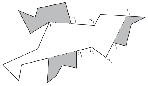
Figure 1: Pocket$(u_{i},v_{i}),i=1,2,3$, shaded.

To prove that the visibility graph of a polygon is 2-dismantlable we prove that a maximal pocket in the polygon provides a visibility-increasing edge and that every nonconvex polygon has at least two maximal pockets.

Lemma 2.

If $uv$ is an edge of a polygon and Pocket$(u,v)$ is maximal then $uv$ is a visibility-increasing edge.

Aichholzer et al. [1, Lemma 2] essentially proved this although it was not expressed in terms of maximal pockets. Also they assumed the polygon has no three collinear vertices. We include a proof.

Proof.

We prove the contrapositive. Suppose that edge $uv$ is not visibility-increasing. If $u$ is a reflex vertex with next neighbour $w$, say, then Pocket$(w,u)$ properly contains Pocket$(u,v)$, which implies that Pocket$(u,v)$ is not maximal. Thus we may assume that $u$ is convex. Since $uv$ is not visibility-increasing there are two points $p_{1}$ and $p_{2}$ in order along $uv$ such that the visibility polygon of $p_{1}$ is not contained in the visibility polygon of $p_{2}$. Thus there is a point $t$ which is visible to $p_{1}$ but not visible to $p_{2}$. See Fig. 2. By extending the segment $p_{1}t$, we may assume, without loss of generality, that $t$ is on the polygon boundary. We claim that $t$ lies in the closed half-plane bounded by the line through $uv$ and lying on the opposite side of Pocket$(u,v)$. This is obvious if $p_{1}$ is internal to edge $uv$, and if $p_{1}=u$ it follows because $u$ is convex. Furthermore, $t$ cannot lie on the line through $u,v$ otherwise $p_{2}$ would see $t$.

Now move point $p$ from $p_{1}$ to $p_{2}$ stopping at the last point where $p$ sees $t$. See Fig. 2. There must be a reflex vertex $v^{\prime}$ on the segment $tp$. The points $v^{\prime}$ and $t$ divide the polygon boundary into two paths. Take the path that does not contain $v$, and let $u^{\prime}$ be the first neighbour of $v^{\prime}$ along this path. It may happen that $u^{\prime}=t$. Then, as shown in Fig. 2, Pocket$(u^{\prime}v^{\prime})$ properly contains Pocket$(u,v)$, so Pocket$(u,v)$ is not maximal.

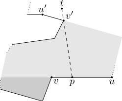
Figure 2: If $uv$ is not visibility-increasing then Pocket$(u,v)$ is not maximal.

∎

Lemma 3.

Any polygon that is not convex has two maximal pockets Pocket($u_{1},v_{1})$ and Pocket$(u_{2},v_{2})$ where $u_{1}$ does not see $u_{2}$.

Proof.

Let Pocket$(u_{1},v_{1})$ be a maximal pocket. Let $u$ be the other neighbour of $v_{1}$ on the polygon boundary. Consider Pocket$(u,v_{1})$, which must be contained in some maximal pocket, Pocket$(u_{2},v_{2})$. Vertex $u_{1}$ is inside Pocket$(u,v_{1})$ and not on the line of its mouth. Therefore $u_{1}$ is inside Pocket$(u_{2},v_{2})$ and not on the line of its mouth. Since $u_{2}$ cannot see points inside Pocket$(u_{2},v_{2})$ except on the line of its mouth therefore $u_{2}$ cannot see $u_{1}$. ∎

From the above lemmas, together with the observation that the visibility graph of a convex polygon is a complete graph, which is 2-dismantlable, we obtain the result that visibility graphs are 2-dismantlable.

Theorem 1.

The visibility graph of a polygon is 2-dismantlable.

Consequently, the cop wins the cops and robbers game on the visibility graph of an $n$-vertex polygon in at most $\frac{n}{2}$ steps. There is a lower bound of $n/4$ cop moves in the worst case, as shown by the skinny zig-zag polygon illustrated in Figure 3. In Section 5.1 we will prove an $\Omega(n)$ lower bound on the number of cop moves even when the cop can move on points interior to the polygon, and even when the polygon has link diameter 3, i.e. any two points in the polygon are joined by a path of at most 3 segments.

Figure 3: An $n$-vertex polygon in which the robber can survive for $n/4$ steps.

5 Cops and Robbers Inside a Polygon

In this section we look at the cops and robbers game on all points inside a polygon. This is a cops and robbers game on an infinite graph so induction on dismantlable orderings does not immediately apply. Instead we give a direct geometric proof that the cop always wins. Although the next section proves more generally that the cop always wins in any simply connected planar region with a reasonable boundary, it is worth first seeing the simpler proof for the polygonal case, both to gain understanding and because this case has a tight $\Theta(n)$ bound on the maximum number of moves (discussed in Section 5.1).

Theorem 2.

The cop wins the cops and robbers game on the points inside any polygon in at most $n$ steps using the strategy of always taking the first segment of the shortest path from its current position to the robber.

Proof.

We argue that each move of the cop restricts the robber to an ever shrinking active region of the polygon. Suppose the cop is initially at $c_{0}$ and the robber initially at $r_{0}$. In the $i^{\rm th}$ move the cop moves to $c_{i}$ and then the robber moves to $r_{i}$.

Observe that for $i\geq 1$ points $c_{i}$ are at reflex vertices of the polygon. To define the active region $P_{i}$ containing the robber position $r_{i}$, we first define its boundary, a directed line segment, $\bar{\ell}_{i}$. Suppose that the shortest path from $c_{i-1}$ to $r_{i-1}$ turns left at $c_{i}$, as in Figure 4. Define $\bar{\ell}_{i}$ to be the segment that starts at $c_{i}$ and goes through $c_{i-1}$ and stops at the first boundary point of the polygon where an edge of the polygon goes to the left of the ray $c_{i}c_{i-1}$. (If the shortest path turns right at $c_{i}$ we similarly define $\bar{\ell}_{i}$ to stop where a polygon edge goes right.) In general, the segment $\bar{\ell}_{i}$ cuts the polygon into two (or more) pieces; let active region $P_{i}$ be the piece that contains $r_{i-1}$. (In the very first step, $\bar{\ell}_{1}$ may hug the polygon boundary, so $P_{1}$ may be all of $P$.)

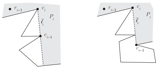
Figure 4: The segment $\bar{\ell}_{i}$ and the active region $P_{i}$ (shaded) containing robber positions $r_{k}$, for all $k\geq i-1$.

We claim by induction on the (decreasing) number of vertices of $P_{i}$ that the robber can never leave $P_{i}$, i.e., that $r_{i}$, $r_{i+1}$,… are in $P_{i}$. It suffices to show that $r_{i}$ is in $P_{i}$ and that $P_{i+1}\subseteq P_{i}$ and that $P_{i+1}$ has fewer vertices.

Suppose that the shortest path from $c_{i-1}$ to $r_{i-1}$ turns left at $c_{i}$. (The other case is completely symmetric.) Observe that the next robber position $r_{i}$ must be inside $P_{i}$, i.e., the robber cannot move from $r_{i-1}$ to cross $\bar{\ell}_{i}$. We distinguish two cases depending whether the shortest path from $c_{i}$ to $r_{i}$ makes a left or a right turn at $c_{i+1}$.

Case 1. See Figure 5. The shortest path from $c_{i}$ to $r_{i}$ makes a left turn at $c_{i+1}$. We consider two subcases: (a) $c_{i+1}$ is left of the ray $c_{i-1}c_{i}$; and (b) $c_{i+1}$ is right of (or on) the ray $c_{i-1}c_{i}$. We claim that case (b) cannot happen because the robber could not have moved from $r_{i-1}$ to $r_{i}$—see Figure 5(b). For case (a) observe that $\bar{\ell}_{i+1}$ extends past $c_{i}$ and therefore $P_{i+1}$ is a subset of $P_{i}$ and smaller by at least one vertex—see Figure 5(a).

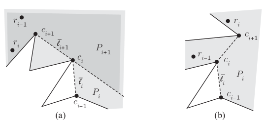
Figure 5: Case 1. (a) If $c_{i+1}$ is left of the ray $c_{i-1}c_{i}$ then $P_{i+1}$ (darkly shaded) is a subset of $P_{i}$ (lightly shaded). (b) It cannot happen that $c_{i+1}$ is to the right of the ray $c_{i-1}c_{i}$ because the robber could not have moved from $r_{i-1}$ to $r_{i}$.

Case 2. See Figure 6. The shortest path from $c_{i}$ to $r_{i}$ makes a right turn at $c_{i+1}$. We consider two subcases: (a) $c_{i+1}$ is left of the ray $c_{i-1}c_{i}$; and (b) $c_{i+1}$ is right of (or on) the ray $c_{i-1}c_{i}$. See Figure 6. In case (a) $\bar{\ell}_{i+1}$ stops at $c_{i}$ and in case (b) it may happen that $\bar{\ell}_{i+1}$ extends past $c_{i}$, but in either case, segment $\bar{\ell}_{i}$ is outside $P_{i+1}$, and $P_{i+1}$ is a subset of $P_{i}$ and smaller by at least one vertex. ∎

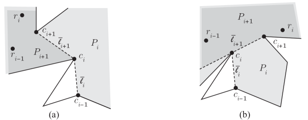
Figure 6: Case 2. (a) $c_{i+1}$ is left of the ray $c_{i-1}c_{i}$. (b) $c_{i+1}$ is right of the ray $c_{i-1}c_{i}$. In either case $P_{i+1}$ (darkly shaded) is a subset of $P_{i}$ (lightly shaded).

We note that Bhadauria et al. [6] use the same cop strategy of following a shortest path to the robber for the version of the problem where each cop or robber move is at most distance 1.

Theorem 2 can alternatively be proved by decomposing the polygon into $O(n^{2})$ triangular regions and proving that they have an ordering with properties like a dismantlable ordering, but we do not include the proof here.

5.1 Lower Bounds

In this subsection we discuss lower bounds on the worst case number of cop moves. The example in Figure 3 shows that the cop may need $\Omega(n)$ moves even when it may move on interior points of the polygon. We give an example to show that this lower bound holds even when the polygon has small link diameter.

Theorem 3.

There is an $n$-vertex polygon with link diameter 3 and a robber strategy that forces the cop to use $\Omega(n)$ steps.

Figure 7: A polygon with constant link diameter in which the robber can survive for $\Omega(n)$ steps.

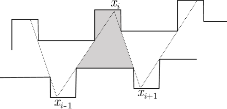
Figure 8: We can adjust the edges and the dashed-line path such that the polygon becomes non-degenerate.

Proof.

We modify the zig-zag polygon from Figure 3 to decrease the link diameter to 3 as shown in Figure 7. The polygon consists of $k=n/3$ similar sections concatenated, where $n$ is the number of vertices of the polygon. We will show that the robber has a strategy to survive at least $k/2$ steps in such a polygon.

Robber Strategy: The robber plays on points $x_{i}$, $1\leq i\leq k$. Initially the robber chooses the closest point $x_{i}$ to $x_{\lfloor{k/2}\rfloor}$ such that $x_{i}$ is not visible to the cop’s initial position. Observe that $x_{i}$ is only visible to the gray area in Figure 7 and the line segments $x_{i-1}x_{i}$ and $x_{i}x_{i+1}$, so the cop can only see at most two of the $x_{i}$’s from its initial position.

The robber remains stationary until it is visible to the cop, i.e., when the cop enters the gray area or along the segments $x_{i-1}x_{i}$ and $x_{i}x_{i+1}$. Then, the robber moves to one of the neighbors $x_{i-1}$ or $x_{i+1}$, the one that is not visible to the cop. At least one of $x_{i-1}$ and $x_{i+1}$ is safe for the robber to move to in the next step as we observe that there is no point visible to all three of $x_{i-1}$, $x_{i}$, and $x_{i+1}$. The robber can survive at least $k/2-1$ steps with this strategy as the game may only be terminated at either $x_{1}$ or $x_{k}$.

Note that the polygon in Figure 7 is degenerate, with edges that lie on the same line, but we can adjust it a little bit to resolve all degeneracies, as shown in Figure 8, at the expense of decreasing the lower bound to $n/8$. We need to be careful not to increase the link diameter of the polygon through the edge level changes. The changes in horizontal edge levels must be small in comparison with the width of the middle corridor. ∎

6 Cops and Robbers Inside a Splinegon

In this section we consider the cops and robbers game in a simply connected region with curved boundary, specifically a splinegon $R$ whose boundary consists of $n$ smooth curve segments that each lie on their own convex hull. Other natural assumptions (such as algebraic curves or splines of limited degree, or other curves of constant complexity) give regions that can be converted to splinegons with a constant factor overhead by cutting at points of inflection and points with vertical tangents. Assume that tangents in a given direction and common tangents between curve segments can be computed. A vertex is an endpoint between two curve segments.

We need another assumption to avoid an infinite game where the cop gets closer and closer to the robber but never reaches it. This occurs, for example, when two curves meet tangentially at a vertex as in Figure 9—in fact, in this situation a robber at a vertex avoids capture by remaining stationary. One possibility is to assume that the robber is captured when the cop gets sufficiently close (within some $\epsilon$). Instead, we will make the assumption that the link distance between any two points in the splinegon $R$ is finite, and bounded by $d$.

Figure 9: The number of cop moves may be infinite even when $n=2$. Truncating the vertices makes the game finite but the number of moves may depend on the link diameter.

With these assumption—a splinegon $R$ of $n$ curved segments with link diameter $d$—we prove that the cop always wins, and does so in $O(n^{2}+d)$ steps. But first, we show through additional examples that the strategy must be a little more complex than in the polygonal case.

6.1 The Cop Strategy

A main difference from the polygonal case is that the cop may need to move to interior points in order to win. Figure 10, for example, shows a region in which the robber can win if the cop always stops on the boundary.

Figure 10: If the cop plays only on the boundary then the robber can win: the robber’s strategy is to play on the middle dashed portions of the boundary and always move to the same curve $S_{i}$ that the cop is on. In our cop strategy the cop would move to the endpoint tangents (drawn as thin lines).

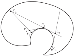
Figure 11: If the cop moves only far enough to see the robber then the robber can win because it can force the cop to take smaller and smaller steps.

Our strategy is that the cop starts off along the first straight segment of the shortest path to the robber’s current position. However, if this segment is tangent to a concave curve of the shortest path then the cop should move further, into the interior of the polygon. How far should the cop go? It is tempting stop the cop when it can see the robber, but Figure 11 shows that this strategy fails—the cop should move farther. Figure 12 shows there is also a danger of moving the cop too far.

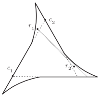
Figure 12: If the cop moves too far then the robber can win: the cop moves from $c_{1}$ to $c_{2}$, the robber moves from $r_{1}$ to $r_{2}$ (dotted line) and then this can be repeated around the polygon. In our proposed strategy the cop would not move from $c_{1}$ all the way to $c_{2}$—it would stop at a robber exit line (drawn as a thin line).

In our strategy the cop will stop at certain lines inside the splinegon. We first state the cop strategy in terms of these lines, and then define the lines. We use the notation $c_{i-1}$ for the cop’s position and $r_{i-1}$ for the robber’s position at the start of round $i$. Their initial positions are $c_{0}$ and $r_{0}$. Recall that each round begins with a cop move.

Cop Strategy for Round $i$. If the cop sees the robber, it moves to the robber’s position and wins. Otherwise, define the cop’s next position, $c_{i}$ as follows: Compute the shortest path from the cop’s current position, $c_{i-1}$, to the robber’s current position, $r_{i-1}$. Let $\ell_{i}$ be the ray along the first straight segment of this shortest path, or, if the shortest path begins with a curve, let $\ell_{i}$ be the tangent to this curve. Let $b_{i}$ be the first point where the shortest path diverges from $\ell_{i}$. Then $b_{i}$ lies on the boundary of the splinegon $R$. If $b_{i}$ is not a splinegon vertex, let $\gamma_{i}$ be the boundary curve containing $b_{i}$. If $b_{i}$ is a splinegon vertex then there are two boundary curves incident to $b_{i}$, and we let $\gamma_{i}$ be the one on the far side of $b_{i}$ with respect to the direction of $\ell_{i}$. By reflection if necessary, assume that the path starts upward and turns left, as depicted in Figure 13.

If $b_{i}\neq c_{i-1}$ and $b_{i}$ is a vertex, then define $c_{i}$ to be $b_{i}$. (This matches the polygonal case.) Otherwise $\ell_{i}$ is tangent to $\gamma_{i}$, so define $c_{i}$ to be the first point on the ray $\ell_{i}$, past $b_{i}$, where $\ell_{i}$ intersects a common tangent or a robber exit line or touches the splinegon boundary.

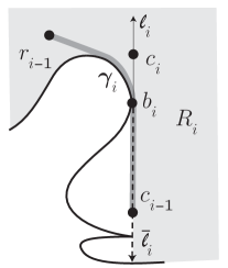
Figure 13: The cop move, showing the shortest path from $c_{i-1}$ to $r_{i-1}$ (thick grey path), the first straight segment of this path $c_{i-1}b_{i}$ upward along ray $\ell_{i}$, the new cop position $c_{i}$, the downward segment $\bar{\ell}_{i}$ (dashed) and the active region $R_{i}$ (lightly shaded).

We now define common tangents and robber exit lines. Refer to Figure 14. A common tangent is a line segment that is tangent to $R$ at two points and extends in both directions until it exits the region. At each endpoint of each curve we have an endpoint tangent—the tangent to the curve through the endpoint. An endpoint tangent extends in both directions until it exits the region. We count endpoint tangents as common tangents. There are $O(n^{2})$ common tangents, because a curve has at most two common tangents with any other curve or vertex.

We define robber exit lines relative to the current robber and cop positions, using the notation from the cop strategy above. See Figure 14. Consider segments that start at $r_{i-1}$ and are tangent to $R$, ending at the tangent point. Among these, a robber exit line is one that crosses ray $\ell_{i}$ such that the tangent point is on the far side of the segment with respect to the direction of $\ell_{i}$. If we extend a robber exit line past its tangent point to the region boundary we obtain a bay of points not visible from the robber position. Note that every bay contains a vertex of the region—either the tangent point itself is a vertex or the tangent point is on a reflex curve, and we must change curves before the end of the bay.

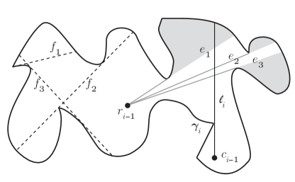
Figure 14: Lines $f_{1},f_{2}$ and $f_{3}$ are three of the many common tangents. Lines $e_{1},e_{2}$ and $e_{3}$ go through $r_{i-1}$ and are tangent to $R$; of those, $e_{2}$ is the only exit line. Lightly shaded regions are the bays.

With these definitions of common tangents and robber exit lines, we have completely specified the cop strategy. We note that the cop’s move can be computed in polynomial time assuming we have constant time subroutines to compute common tangents and tangents at a given point. We can preprocess to find all common tangents. For a given robber position, we can find all robber exit lines in polynomial time. We can find shortest paths in the splinegon $R$ in linear time using the algorithm of [24]. With this information, we can find the next cop position. A straightforward implementation takes $O(n^{2})$ time, though this can probably be improved.

6.2 The Cop Wins

In order to prove that the cop wins using the strategy specified in the previous section, we first show that each cop move restricts the robber to a smaller subregion. Then we show that the number of steps the cop needs to win is $O(n^{2}+d)$ where $n$ is the number of segments and $d$ is the link diameter of the region.

We begin by defining the subregion that the robber is restricted to during and after round $i$. Define $\bar{\ell}_{i}$ to be the directed segment that starts at $b_{i}$, goes opposite ray $\ell_{i}$ through $c_{i-1}$, and stops at the first boundary point for which every $\epsilon>0$ neighborhood contains a boundary point on the opposite side of $\bar{\ell}_{i}$ from $\gamma_{i}$ at $b_{i}$ (i.e., where part of the boundary is to the left of the downward directed segment $\bar{\ell}_{i}$ in Figure 13.) The segment $\bar{\ell}_{i}$ starts and ends on the boundary so it cuts the region into two (or more) pieces; define the active region, $R_{i}$, to be the piece that contains $r_{i-1}$. Define the exclusion region to be its complement in $R$. Observe that the robber cannot exit $R_{i}$ in round $i$, i.e., $r_{i}$ is inside $R_{i}$. This is because $r_{i-1}$ is on the wrong side of the line through $\bar{\ell}_{i}$.

We prove below in Lemma 6 that $R_{i+1}\subsetneq R_{i}$, i.e., the active region shrinks. Following that, we show that the cop wins in a finite number of steps. The proofs are similar to the analogous results for polygons, and involve handling four cases for the left/right configuration of the cop and the robber. Suppose that the shortest path from $c_{i-1}$ to $r_{i-1}$ makes a left turn at $b_{i}$. (The other case is completely symmetric.) We distinguish the following cases:

Case 1. The shortest path from $c_{i}$ to $r_{i}$ makes a left turn at $b_{i+1}$.

(a) $c_{i+1}$ is left of the ray $c_{i-1}c_{i}$—more precisely, in moving from $c_{i-1}$ to $c_{i}$ to $c_{i+1}$ the cop turns left by an angle in the range $(0,180^{\circ})$. (Turning by $0^{\circ}$ will be handled in case (b).)

(b) $c_{i+1}$ is right of the ray $c_{i-1}c_{i}$—more precisely, the cop turns right at $c_{i}$ by an angle in $[0,180^{\circ})$.

Case 2. The shortest path from $c_{i}$ to $r_{i}$ makes a right turn at $b_{i+1}$.

(a) $c_{i+1}$ is left of the ray $c_{i-1}c_{i}$—more precisely, the cop turns left at $c_{i}$ by an angle in $(0,180^{\circ})$.

(b) $c_{i+1}$ is right of the ray $c_{i-1}c_{i}$—more precisely, the cop turns right at $c_{i}$ by an angle in $[0,180^{\circ})$.

Note that the cop never turns by an angle of $180^{\circ}$ (doubling back) because then $b_{i+1}$ would be on the line segment between $c_{i}$ and $b_{i}$ or further along, on the ray $\bar{\ell}_{i}$. In the first case, $b_{i+1}$ would provide a stopping point for $c_{i}$ according to the rule that the cop stops on the boundary. The second case is impossible because the robber can never move from $r_{i-1}$ to a position that would cause the cop to move onto $\bar{\ell}_{i}$.

We begin by showing that Case 2(a) can happen only in special circumstances and that Case 1(b) cannot happen at all.

Lemma 4.

In Case 2(a) the segment $c_{i}b_{i+1}$ is tangent to the boundary on its left side (as well as tangent to the boundary on its right side at $b_{i+1}$).

Proof.

See Figure 15. The segment $c_{i}b_{i+1}$ is tangent to the boundary curve $\gamma_{i+1}$ on its right side at point $b_{i+1}$. Suppose that segment $c_{i}b_{i+1}$ is not tangent to the boundary on its left side. We show that the cop has passed a common tangent, which is a contradiction. Move $c_{i}$ back towards $c_{i-1}$ while maintaining tangency with the curve $\gamma_{i+1}$. We can move some positive amount. Either we reach the tangent at an endpoint of $\gamma_{i+1}$ or the segment $c_{i}b_{i+1}$ hits a boundary point on its left side (possibly because $c_{i}$ reaches $b_{i}$). In either case, we have arrived at a common tangent, so $c_{i}$ should have been placed here rather than further along. ∎

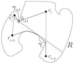
Figure 15: In case 2(a) if the segment $c_{i}b_{i+1}$ is not tangent to the boundary on its left side then there is an earlier choice for $c_{i}$ (on the dashed red common tangent).

Lemma 5.

Case 1(b) cannot occur, i.e., it cannot happen that the shortest path from $c_{i}$ to $r_{i}$ makes a left turn at $b_{i+1}$ and $c_{i+1}$ is right of the ray $c_{i-1}c_{i}$ by an angle in $[0,180^{\circ})$.

Proof.

Suppose the situation does occur. See Figure 16. We show that the cop has passed a common tangent or a robber exit line, which gives a contradiction. Because $c_{i+1}$ is to the right of the ray $c_{i-1}c_{i}$, therefore the robber’s move $r_{i-1}r_{i}$ must have crossed the line through $c_{i-1}c_{i}$, say at point $x$. We claim that segments $r_{i-1}r_{i}$ and $c_{i-1}c_{i}$ intersect. First note that $x$ lies after $b_{i}$ along the ray $c_{i-1}c_{i}$. We must show that $c_{i}$ lies after $x$ along this ray. If $c_{i}$ lies before $x$, then there is a two-link path inside the region, $c_{i},x,r_{i}$ that turns right at $x$. Shortening this to a locally shortest path, we obtain the shortest path from $c_{i}$ to $r_{i}$ that makes a first turn to its right, contradicting our assumption.

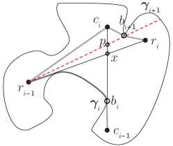
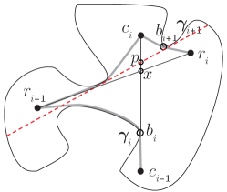
Figure 16: Case 1(b) cannot occur in these situations: moving $p$ from $c_{i}$ towards $b_{i}$ while maintaining tangency of $\tau$ (dashed red) with $\gamma_{i+1}$ we encounter: 16 a robber exit line or 16 a common tangent.

Define $\sigma$ to be the shortest path from $r_{i-1}$ to $c_{i}$. The segment $c_{i}b_{i+1}$ is tangent to the curve $\gamma_{i+1}$. We will now move point $p$ from $c_{i}$ towards $b_{i}$, maintaining a segment $\tau$ through $p$ tangent to the curve $\gamma_{i+1}$. In the other direction, $\tau$ extends to its intersection point with $\sigma$. See Figures 16 and 17, where $\tau$ is drawn as a dashed red line. If $\tau$ reaches an endpoint tangent of $\gamma_{i+1}$ then we have a common tangent and the cop should have stopped at point $p$. Otherwise, the segment $\tau$ must at some point lose contact with $\sigma$ and we claim that this can happen only because of one of the following:

• The segment $\tau$ intersects $\sigma$ at $r_{i-1}$; this is a robber exit line. See Figure 16.

• The segment $\tau$ becomes tangent to $\sigma$; this is a common tangent. See Figure 16.

• The segment bumps into the region boundary (possibly at point $b_{i}$); this is a common tangent. See Figure 17.

In all cases, the cop should have stopped at point $p$ because of the common tangent or robber exit line $\tau$. ∎

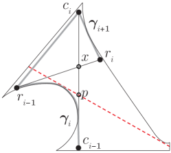
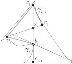
Figure 17: Case 1(b) cannot occur in these situations: moving $p$ from $c_{i}$ towards $b_{i}$ while maintaining tangency of $\tau$ (dashed red) with $\gamma_{i+1}$ we encounter a common tangent by bumping into the region boundary 17 before $p$ reaches $b_{i}$, or 17 at $b_{i}$.

We are now ready to show that the active region shrinks.

Lemma 6.

The active regions satisfy $R_{i+1}\subsetneq R_{i}$.

Proof.

Assume that the shortest path from $c_{i-1}$ to $r_{i-1}$ makes a left turn at $b_{i}$, and consider the cases as listed above.

Case 1(a). The shortest path from $c_{i}$ to $r_{i}$ makes a left turn at $b_{i+1}$ and $c_{i+1}$ is left of the ray $c_{i-1}c_{i}$. See Figure 18. The ray $\bar{\ell}_{i+1}$ from $b_{i+1}$ through $c_{i}$ intersects $\ell_{i}$ at $c_{i}$, and is therefore completely contained in the active region $R_{i}$. Furthermore, the open segment $c_{i-1}c_{i}$ is outside $R_{i+1}$ but inside $R_{i}$. Thus $R_{i+1}\subsetneq R_{i}$.

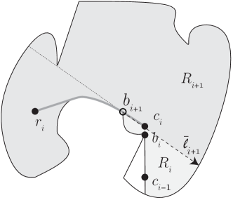
Figure 18: Case 1(a).

Case 1(b). The shortest path from $c_{i}$ to $r_{i}$ makes a left turn at $b_{i+1}$ and $c_{i+1}$ is right of the ray $c_{i-1}c_{i}$. This case cannot occur by Lemma 5.

Case 2(a). The shortest path from $c_{i}$ to $r_{i}$ makes a right turn at $b_{i+1}$ and $c_{i+1}$ is left of the ray $c_{i-1}c_{i}$. See Figure 19. By Lemma 4, the segment $c_{i}b_{i+1}$ is tangent to the boundary on its left side, say at point $p$. The ray $\bar{\ell}_{i+1}$ that defines the active region extends from $b_{i+1}$ to $p$. It’s extension goes through $c_{i}$, so it is contained in $R_{i}$. Furthermore, the open segment $c_{i-1}c_{i}$ is outside $R_{i+1}$ but inside $R_{i}$. Therefore $R_{i+1}\subsetneq R_{i}$.

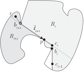
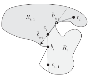
Figure 19: 19 Case 2(a). 19 Case 2(b).

Case 2(b). The shortest path from $c_{i}$ to $r_{i}$ makes a right turn at $b_{i+1}$ and $c_{i+1}$ is right of the ray $c_{i-1}c_{i}$ (or on the ray). See Figure 19. The ray $\bar{\ell}_{i+1}$ intersects $\ell_{i}$ at $c_{i}$, and is contained in $R_{i}$. Furthermore, the open segment $c_{i-1}c_{i}$ is outside $R_{i+1}$ but inside $R_{i}$. Thus $R_{i+1}\subsetneq R_{i}$. ∎

Finally we prove our main result.

Theorem 4.

Inside a splinegon of $n$ curve segments with link diameter $d$, the cop wins the cops and robbers game in $O(n^{2}+d)$ moves.

Proof.

We argue that at each step between the first and the last, the active region shrinks in some discrete way. Define the newly excluded region, $E_{i}$, to be $R_{i}-R_{i+1}$. In order to take care of collinearities, we will include the boundary of $R_{i+1}$ but exclude the boundary of $R_{i}$. If the two boundaries intersect, the intersection point is not included in $E_{i}$. In Figures 18, 19, and 19 the region $E_{i}$ is lightly shaded. By Lemma 6, the $E_{i}$’s are disjoint.

Let $\sigma$ be a minimum link path from the initial to the final cop position. Then $\sigma$ has at most $d$ bends. Note that there are at most $n^{2}$ common tangents because there are at most $n^{2}$ pairs of points determining common tangents. Our bounds derive from these two facts.

Our plan is to show that at each step we make progress in one of the following ways:

1. $c_{i}$ is a vertex

2. $c_{i}$ and $b_{i}$ define a common tangent

3. $E_{i}$ contains a vertex of the region

4. $E_{i}$ contains an endpoint of a common tangent with both endpoints in $R_{i}$

5. $E_{i}$ contains a bend of $\sigma$

We begin by bounding the number of events of each of the above types. After that we will show that one of these events occurs in each step.

Because $c_{i}$ and $b_{i}$ never repeat, event (1) happens at most $n$ times and event (2) happens at most $n^{2}$ times. Because the $E_{i}$’s are disjoint, event (3) happens at most $n$ times, event (4) happens at most $n^{2}$ times, and event (5) happens at most $d$ times.

It remains to prove that at each step, one of the above 5 events occurs.

Recall the conditions for defining the cop’s position $c_{i}$. If $c_{i}=b_{i}$ because $b_{i}$ is a vertex then we have event (1). Otherwise $c_{i}$ stops at a common tangent or a robber exit line or on the boundary of the region.

Suppose first that $c_{i}$ stops on a common tangent, and not on the boundary (we will handle that case below). Note that the common tangent must cross $\ell_{i}$, and therefore that both endpoints of the common tangent lie in $R_{i}$. The boundary of $R_{i+1}$ is a line segment that goes through $c_{i}$ and therefore one endpoint of the common tangent must lie in $R_{i+1}$, possibly in the boundary. This endpoint is in $E_{i}$. Thus we have event (4).

If $c_{i}$ stops on a robber exit line then we claim that $E_{i}$ contains a vertex, i.e., event (3). To justify this, first note that $r_{i-1}$ must lie in $R_{i+1}$. This is because a straight segment joins $r_{i}$ and $r_{i-1}$ and $r_{i}$ lies on the far side of $\ell_{i+1}$, so in order for a straight segment from $r_{i}$ to exit $R_{i+1}$ it would have to cross $\ell_{i+1}$ and $\bar{\ell}_{i+1}$ which is impossible. Therefore the robber exit line must exit $R_{i+1}$ at $c_{i}$ (or possibly lie in the line of $\ell_{i+1}$), and thus the tangent point of the robber exit line, and its bay, must lie in $E_{i}$. As noted when we defined robber exit lines, this bay contains a vertex. Therefore $E_{i}$ contains a vertex.

Finally, we must consider the possibility that $c_{i}$ stops on the region boundary. When can this happen? By Lemma 4, the cop always stops at a common tangent in Case 2(a). By Lemma 5, Case 1(b) never occurs. Thus we must be in Case 1(a) or 2(b). If $c_{i}$ is not at a point where $\ell_{i}$ exits the region then $c_{i}$ and $b_{i}$ define a common tangent, i.e. event (2). We are left with the case where $c_{i}$ is at a point where $\ell_{i}$ exits the region. In Case 2(b) (see Figure 19) the robber’s move $r_{i-1}r_{i}$ must cross line $\ell_{i}$ beyond $c_{i}$, which is impossible if $\ell_{i}$ exits the region at $c_{i}$. Thus we must be in Case 1(a). See Figure 20. The minimum link path $\sigma$ from the initial cop position (outside $R_{i}$, or possibly on the boundary of $R_{i}$) to the final robber position (inside $R_{i+1}$) must include a bend point in $E_{i}$. This is event (5). ∎

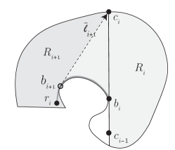
Figure 20: When the cop stops on the region boundary in Case 1(a).

7 Open Problems

1. Consider the cops and robbers game on the points inside a polygonal region, i.e., a polygon with holes. There is a lower bound of three cops—an example requiring three cops can be constructed from a planar graph where three cops are required [2] by taking a straight-line planar drawing of the graph and cutting out polygonal holes to leave narrow corridors for the graph edges. It is an open question whether three cops suffice.

2. What is the complexity of finding how many moves the cop needs for a given polygon/region? The graph version of this problem is solvable in polynomial time for cop-win graphs [20]. For the cops and robbers game on the points inside a polygon we conjecture that the problem is solvable in polynomial time if the cop is restricted to the reflex vertices of the polygon. However, the cop may save by moving to an interior point—for example in a star-shaped polygon whose kernel is disjoint from the polygon boundary—so the problem seems harder if the cop is unrestricted.

3. Is there a lower bound of $\Omega(n^{2}+d)$ on the worst case number of cop moves in a splinegon of $n$ curve segments and link diameter $d$? From results in Section 5.1 we have a lower bound of $\Omega(n+d)$.

8 Acknowledgements

The cops and robbers problem for points inside a region with a curved boundary was initially suggested by Vinayak Pathak and was posed in the Open Problem Session of CCCG 2013 by the third author of this paper. We thank all who participated in discussing the problem, especially David Eppstein.

References

- [1] O. Aichholzer, G. Aloupis, E. D. Demaine, M. L. Demaine, V. Dujmovic, F. Hurtado, A. Lubiw, G. Rote, A. Schulz, D. L. Souvaine, and A. Winslow. Convexifying polygons without losing visibilities. In Canadian Conference on Computational Geometry (CCCG), 2011.
- [2] M. Aigner and M. Fromme. A game of cops and robbers. Discrete Applied Mathematics, 8(1):1–12, 1984.
- [3] B. Alspach. Searching and sweeping graphs: a brief survey. Le Matematiche, 59:5–37, 2004.
- [4] W. Baird and A. Bonato. Meyniel’s conjecture on the cop number: a survey. Journal of Combinatorics, 3:225–238, 2012.
- [5] A. Beveridge, A. Dudek, A. M. Frieze, and T. Müller. Cops and robbers on geometric graphs. Combinatorics, Probability & Computing, 21(6):816–834, 2012.
- [6] D. Bhadauria, K. Klein, V. Isler, and S. Suri. Capturing an evader in polygonal environments with obstacles: The full visibility case. The International Journal of Robotics Research, 31(10):1176–1189, 2012.
- [7] A. Bonato, P. A. Golovach, G. Hahn, and J. Kratochvíl. The capture time of a graph. Discrete Mathematics, 309(18):5588–5595, 2009.
- [8] A. Bonato and R. J. Nowakowski. The Game of Cops and Robbers on Graphs. American Mathematical Society, 2011.
- [9] D. Z. Chen, J. Hershberger, and H. Wang. Computing shortest paths amid convex pseudodisks. SIAM J. Comput., pages 1158–1184, 2013.
- [10] D. Z. Chen and H. Wang. Computing shortest paths among curved obstacles in the plane. In Proceedings of the Twenty-ninth Annual Symposium on Computational Geometry, SoCG ’13, pages 369–378, New York, NY, USA, 2013. ACM.
- [11] T. H. Chung, G. A. Hollinger, and V. Isler. Search and pursuit-evasion in mobile robotics. Autonomous Robots, 31:299–316, 2011.
- [12] D. Dobkin and D. Souvaine. Computational geometry in a curved world. Algorithmica, 5(1-4):421–457, 1990.
- [13] F. V. Fomin, P. A. Golovach, and J. Kratochvíl. On tractability of cops and robbers game. In Fifth IFIP International Conference On Theoretical Computer Science, pages 171–185, 2008.
- [14] F. V. Fomin and D. M. Thilikos. An annotated bibliography on guaranteed graph searching. Theoretical Computer Science, 399(3):236 – 245, 2008.
- [15] S. K. Ghosh. Visibility algorithms in the plane. Cambridge University Press, 2007.
- [16] S. K. Ghosh and P. P. Goswami. Unsolved problems in visibility graphs of points, segments and polygons. CoRR, abs/1012.5187, 2010.
- [17] A. S. Goldstein and E. M. Reingold. The complexity of pursuit on a graph. Theoretical Computer Science, 143(1):93–112, 1995.
- [18] L. J. Guibas, J.-C. Latombe, S. M. Lavalle, D. Lin, and R. Motwani. A visibility-based pursuit-evasion problem. International Journal of Computational Geometry & Applications, 09(4 & 5):471–493, 1999.
- [19] G. Hahn. Cops, robbers and graphs. Tatra Mt. Math. Publ., 36:163–176, 2007.
- [20] G. Hahn and G. MacGillivray. A note on k-cop, l-robber games on graphs. Discrete Mathematics, 306(19-20):2492–2497, 2006.
- [21] J. Hershberger, S. Suri, and H. Yildiz. A near-optimal algorithm for shortest paths among curved obstacles in the plane. In Proceedings of the Twenty-ninth Annual Symposium on Computational Geometry, SoCG ’13, pages 359–368, New York, NY, USA, 2013. ACM.
- [22] V. Isler, S. Kannan, and S. Khanna. Randomized pursuit-evasion in a polygonal environment. IEEE Transactions on Robotics, 21(5):875–884, 2005.
- [23] J. Littlewood. Littlewood’s Miscellany. Cambridge University Press, 1986.
- [24] E. Melissaratos and D. Souvaine. Shortest paths help solve geometric optimization problems in planar regions. SIAM Journal on Computing, 21(4):601–638, 1992.
- [25] R. J. Nowakowski and P. Winkler. Vertex-to-vertex pursuit in a graph. Discrete Mathematics, 43(2-3):235–239, 1983.
- [26] A. Quilliot. Homomorphismes, points fixes dans les graphes, les ensembles ordonnés et les espaces métriques. Ph. D. Thesis, These de Doctorat d’Etat, Université de Paris VI, 1983.
- [27] P. D. Seymour and R. Thomas. Graph searching and a min-max theorem for tree-width. Journal of Combinatorial Theory, Series B, 58(1):22–33, 1993.
- [28] T. Shermer. Recent results in art galleries. Proceedings of the IEEE, 80(9):1384–1399, 1992.