The isotope effect in ${\rm H_{3}S}$ superconductor

Abstract

The experimental value of ${\rm H_{3}S}$ isotope coefficient decreases from $2.37$ to $0.31$ in the pressure range from $130$ GPa to $200$ GPa. We have shown that the value of $0.31$ is correctly reproduced in the framework of the classical Eliashberg approach. On the other hand, the anomalously large value of the isotope coefficient ($2.37$) may be associated with the strong renormalization of the normal state by the electron density of states.

Keywords: ${\rm H_{3}S}$ and ${\rm D_{3}S}$ superconductor, isotope coefficient, Eliashberg approach.

The metallic hydrogen the most probably could be the superconductor with the very high value of the critical temperature ($T_{C}$) Wigner and Huntington (1935), Ashcroft (1968). The expected high $T_{C}$ is associated with the large Debye frequency (the mass of the proton is very small) and the lack of the electrons on the inner shells, which should significantly increase the electron-phonon coupling constant ($\lambda$) Cudazzo et al. (2008), Szczȩśniak and Jarosik (2009), McMahon and Ceperley (2011). Unfortunately, the pressure of the hydrogen’s metallization is very large ($p>400$ GPa Narayana et al. (1998), Stadele and Martin (2000)). For this reason, the experimental confirmation of the theoretical predictions has not been obtained to this day.

In 2004 Ashcroft suggested the existence of the superconducting state in the hydrogen-rich compounds with the critical temperature comparable to $T_{C}$ of the pure hydrogen, whereas the metallization pressure might be subjected to the significant decrease due to the existence of the chemical pre-compression Ashcroft (2004). Ashcroft’s predictions were confirmed in many later papers. The selected results are presented in Fig. 1.

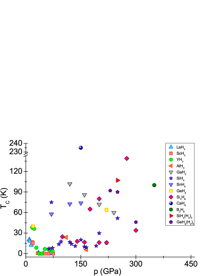
Figure 1: The predicted critical temperatures for the hydrogen-rich compounds. The results for tri-hydrides: LaH₃, ScH₃, YH₃, AlH₃, and GaH₃ are from works Kim et al. (2010), Goncharenko et al. (2008), and Gao et al. (2011). The results obtained for four-hydrides are presented in the papers: SiH₄ Eremets et al. (2008) (experiment), Martinez-Canales et al. (2009), Chen et al. (2008), SnH₄ Tse et al. (2007), GeH₄ Gao et al. (2008). The results for six-hydrides and eight-hydrides were obtained in works Si₂H₆ Jin et al. (2010), Flores-Livas et al. (2012), $\rm Ba_{2}H_{6}$ Abe and Ashcroft (2011), $\rm CaH_{6}$ Wang et al. (2012), SiH₄(H₂)₂ Li et al. (2010), and GeH₄(H₂)₂ Zhong et al. (2012), Zhong et al. (2013).

The superconducting state in the hydrogen sulfide with the exceptionally high value of the critical temperature ($T_{C}\sim 200$ K) was discovered in 2014 Drozdov et al. (2014), Drozdov et al. (2015). The detailed dependence of the critical temperature on the pressure for the compounds ${\rm H_{3}S}$ and ${\rm D_{3}S}$ is presented in Fig. 2.

Figure 2: The influence of the pressure on the value of the critical temperature - ${\rm H_{3}S}$ (the red circles) and ${\rm D_{3}S}$ (the green circles) Einaga et al. (2015). The lines were obtained using the approximation procedure. The squares represent the results obtained with the help of the classical Eliashberg equations in the harmonic approximation, the triangle represents the anharmonic analysis, and the blue spheres denote expression (5).

The experimental results Drozdov et al. (2014), Drozdov et al. (2015) and the theoretical papers Duan et al. (2014); Li et al. (2014); Durajski et al. (2015a, b); Bianconi and Jarlborg (2015a); Ortenzi et al. (2015) suggest that the superconducting state in the hydrogen sulfide is induced by the electron-phonon interaction. In particular, the strong isotope effect was observed. However, the values of the isotope coefficient ($\alpha$) significantly differ from the canonical value of $0.5$ predicted by the BCS theory Bardeen et al. (1957a), Bardeen et al. (1957b).

In the presented paper, we explained the experimental data for $\alpha$ on the basis of the classical and the extended Eliashberg formalism basing on the phonon pairing mechanism.

In the first step, on the basis of the experimental results, we determined the approximation lines $T^{\rm H_{3}S}_{C}\left(p\right)$ and $T^{\rm D_{3}S}_{C}\left(p\right)$ which served for the calculation of the isotope coefficient:

$$\alpha_{\rm exp}\left(p\right)=-\frac{\ln\left[T^{\rm D_{3}S}_{C}\left(p\right)\right]-\ln\left[T^{\rm H_{3}S}_{C}\left(p\right)\right]}{\ln\left[m_{\rm D}\right]-\ln\left[m_{\rm H}\right]},$$ (1)

where $m_{\rm D}$ and $m_{\rm H}$ are respectively the deuterium’s and protium’s atomic mass. The shape of the function $\alpha_{\rm exp}\left(p\right)$ is plotted in Fig. 3. It can be clearly seen that the isotope coefficient decreases with the increasing pressure. In particular, the following values were obtained: $\alpha_{\rm exp}\left(130\hskip 2.84526pt{\rm GPa}\right)=2.37$ and $\alpha_{\rm exp}\left(200\hskip 2.84526pt{\rm GPa}\right)=0.31$.

Figure 3: The blue line - the experimental values of the isotope coefficient on the basis of formula (1). The squares were obtained in the framework of the classical Eliashberg formalism in the harmonic approximation. The triangle corresponds to the classical Eliashberg formalism - the anharmonic analysis. The red circle was obtained assuming the strong renormalization of the normal state by the electron density of states.

The value of the isotope coefficient for $p=200$ GPa can be reproduced in the framework of the classical Eliashberg formalism. To this end, we solved numerically equations Eliashberg (1960), Szczȩśniak (2006):

$$\varphi_{n}=\frac{\pi}{\beta}\sum_{m=-1100}^{1100}\frac{K\left(i\omega_{n}-i\omega_{m}\right)-\mu^{\star}\left(\omega_{m}\right)}{\sqrt{\omega_{m}^{2}Z^{2}_{m}+\varphi^{2}_{m}}}\varphi_{m},$$ (2)

$$Z_{n}=1+\frac{1}{\omega_{n}}\frac{\pi}{\beta}\sum_{m=-1100}^{1100}\frac{\lambda\left(i\omega_{n}-i\omega_{m}\right)}{\sqrt{\omega_{m}^{2}Z^{2}_{m}+\varphi^{2}_{m}}}\omega_{m}Z_{m},$$ (3)

where $\varphi_{n}=\varphi\left(i\omega_{n}\right)$ represents the order parameter function, and $Z_{n}=Z\left(i\omega_{n}\right)$ denotes the wave function renormalization factor. The fermion Matsubara frequency is given by the formula: $\omega_{n}=\frac{\pi}{\beta}\left(2n-1\right)$, $\beta=1/k_{B}T$ ($k_{B}$ is the Boltzmann constant). The electron-phonon pairing kernel has the following form: $K\left(z\right)=2\int_{0}^{+\infty}d\Omega\frac{\Omega}{\Omega^{2}-z^{2}}\overline{\alpha}^{2}F\left(\Omega\right)$. The Eliashberg functions ($\overline{\alpha}^{2}F\left(\Omega\right)$) for $p=130$ GPa and $p=200$ GPa were calculated by Duan et al. Duan et al. (2014).

The depairing electron correlations in the Eliashberg formalism are described with the use of the formula: $\mu^{\star}\left(\omega_{n}\right)=\mu^{\star}\theta\left(\omega_{C}-|\omega_{n}|\right)$. The quantity $\mu^{\star}$ denotes the Coulomb pseudopotential, $\theta$ is the Heaviside function. $\omega_{C}$ represents the cut-off frequency: $\omega_{C}=3\Omega_{\rm{max}}$, where $\Omega_{\rm{max}}$ is the Debye frequency. It should be noted that the Coulomb pseudopotential was defined by Morel and Anderson Morel and Anderson (1962):

$$\mu^{\star}=\frac{\mu}{1+\mu\ln\left(\frac{\omega_{e}}{\omega_{\rm ln}}\right)}.$$ (4)

The symbol $\mu$ is given by the formula: $\mu=\rho\left(0\right)U$, whereas $\rho\left(0\right)$ is the value of the electron density of states at the Fermi level, and $U$ is the Coulomb integral. The quantity $\omega_{e}$ represents the characteristic electron frequency and the logarithmic phonon frequency is given by: $\omega_{{\rm ln}}=\exp\left[\frac{2}{\lambda}\int^{\Omega_{\rm{max}}}_{0}d\Omega\frac{\overline{\alpha}^{2}\left(\Omega\right)F\left(\Omega\right)}{\Omega}\ln\left(\Omega\right)\right]$.

In Fig. 2, we marked the values of the critical temperature calculated with the help of the Eliashberg equations. We considered $\mu^{\star}\in\{0.1,0.2,0.3\}$. Additionally, we also placed the value of $T_{C}$ for $p=200$ GPa, determined beyond the harmonic approximation Errea et al. (2015). It turns out that the numerical results can be reproduced using the formula (see also Fig. 1):

$$k_{B}T_{C}=\omega_{{\rm ln}}\exp\left[\frac{-\left(1+\lambda\right)}{\lambda-\mu^{\star}\left(1+0.4369\lambda\right)}\right],$$ (5)

where the electron-phonon coupling constant should be calculated from: $\lambda=2\int^{\Omega_{\rm{max}}}_{0}d\Omega\frac{\overline{\alpha}^{2}\left(\Omega\right)F\left(\Omega\right)}{\Omega}$.

On this basis, it was found out that the values $\mu^{\star}$ corresponding to $\left[T_{C}\right]_{\rm exp}$ were equal to $0.239$ and $0.286$, respectively for the pressure at $130$ GPa and $200$ GPa (the harmonic approximation), and $0.146$ (the anharmonic analysis).

The expression on the isotope coefficient was derived using the dependence:

$$\alpha=\frac{\omega_{\rm ln}}{2T_{C}}\frac{dT_{C}}{d\omega_{\rm ln}}.$$ (6)

Thus:

$$\alpha=\frac{1}{2}\left[1-\frac{\left(1+\lambda\right)\left(1+0.4369\lambda\right)\left(\mu^{\star}\right)^{2}}{\left(\lambda-\mu^{\star}\left(1+0.4369\lambda\right)\right)^{2}}\right].$$ (7)

The theoretical results have the following form: $\alpha\left(130\hskip 2.84526pt{\rm GPa}\right)=0.432$ and $\alpha\left(200\hskip 2.84526pt{\rm GPa}\right)=0.397$ (the harmonic approximation), and $\alpha\left(200\hskip 2.84526pt{\rm GPa}\right)=0.477$ (the anharmonic approach). It can be easily seen that the theoretical value of the isotope coefficient for $p=200$ GPa in harmonic approximation qualitatively well reproduce the experimental data. In the case of $p=130$ GPa the discrepancy between the Eliashberg result and the result of the measure is extremely high, which means the collapse of the classical theoretical description.

The high value of the isotope coefficient in the terms of the lower pressures can be tried to explain by the pairing mechanism other than the electron-phonon mechanism Hirsch and Marsiglio (2015). However, the modifying of the classical Eliashberg formalism should also be considered. From the theoretical point of view it highlights the big change of the electron density of states at and near the Fermi surface together with the pressure change. The ab initio calculations performed for $p=210$ GPa suggest the existence of the sharp peak of $\rho\left(\varepsilon\right)$ very close to the Fermi surface Papaconstantopoulos et al. (2015). The peak moves away from the Fermi surface and vanishes for the lower pressures Duan et al. (2014), Li et al. (2014), Bianconi and Jarlborg (2015b). Hence, physically this means the significant modification of the normal state in the studied system.

Let us consider the renormalized Green function of the normal state, in which the depreciation of the electron density of states was taken into account Szczȩśniak et al. (2001):

$$G_{\mbox{{\scriptsize{\bf k}}}}\left(i\omega_{n}\right)=-\frac{i\omega_{n}\tau_{0}+\varepsilon_{\mbox{{\scriptsize{\bf k}}}}\tau_{3}}{\omega_{n}^{2}+\varepsilon_{\mbox{{\scriptsize{\bf k}}}}^{2}+B^{2}}A-\frac{i\omega_{n}\tau_{0}+\varepsilon_{\mbox{{\scriptsize{\bf k}}}}\tau_{3}}{\omega_{n}^{2}+\varepsilon_{\mbox{{\scriptsize{\bf k}}}}^{2}}\left(1-A\right),$$ (8)

where $\tau_{0}$, $\tau_{3}$ are the Pauli matrices associated with the normal state and $\varepsilon_{\mbox{{\scriptsize{\bf k}}}}$ is the electron energy. The parameters $A\in\left<0,1\right>$ and $B$ determine the depth and the width of the decrease in electron density of states with respect to the baseline at the Fermi level. Deriving the Eliashberg equations for the renormalized Green function and using the approximations discussed in paper Szczȩśniak et al. (2001), the algebraic equation on the critical temperature can be obtained:

$$1=\frac{\lambda}{1+\lambda}\ln\left(\frac{\omega_{\ln}}{2\pi k_{B}T_{C}}\right)-\frac{\lambda}{1+\lambda}\left[f_{1}\Psi\left(\frac{1}{2}\right)+2f_{2}{\rm Re}\Psi\left(\frac{1}{2}+\frac{iB}{2\pi k_{B}T_{C}}\right)+2f_{3}{\rm Re}\Psi\left(\frac{1}{2}+\frac{igB}{2\pi k_{B}T_{C}}\right)\right],$$ (9)

where:

$$g=\left[\frac{\left(1-A\right)\left(1+\lambda\right)+A}{1+\lambda}\right]^{1/2},$$ (10)

$$f_{1}=\frac{\left(1-A\right)^{2}}{g^{2}},$$ (11)

$$f_{2}=\frac{1}{2g^{2}}\left[g^{2}-\left(1-A\right)^{2}+\frac{\left(1-A-g^{2}\right)^{2}}{1-g^{2}}\right],$$ (12)

$$f_{3}=-\frac{1}{2g^{2}}\left[\frac{\left(1-A-g^{2}\right)^{2}}{1-g^{2}}\right].$$ (13)

The symbol $\Psi$ denotes the digamma function.

We solved numerically equation (9) assuming the input parameters for the pressure at $130$ GPa. It turns out that equation (9) allows to reproduce the experimental values of the critical temperature and the isotope coefficient for $A=0.904$ and $B=29.12$ meV. Physically this means the very sharp drop in the electron density of states at and near the Fermi level in the narrow energy range. The obtained result in the natural manner can be associated with the offset of the $\rho\left(\varepsilon\right)$ peak from the Fermi surface.

In conclusion, basing on the experimental data we determined the range of variation of the isotopic coefficient for ${\rm H_{3}S}$ superconductor in the function of the pressure. We showed that the isotope coefficient accepts the anomalously high values in the area of the lower pressures ($\sim 130$ GPa). On the other hand, for the higher pressures ($\sim 200$ GPa), the values of $\alpha$ are lower than those in the BCS theory. The conducted theoretical analysis proved that the low values of the isotope coefficient could be reproduced in the framework of the classical Eliashberg formalism. The anomalously high values of $\alpha$ could be induced by the strong renormalization of the normal state associated with the significant changes of the electron density of states with the change in the pressure. Note that the proposed model does not require the non-phonon pairing mechanism.

References

- Wigner and Huntington (1935) E. Wigner and H. B. Huntington, The Journal of Chemical Physics 3, 764 (1935).
- Ashcroft (1968) N. W. Ashcroft, Physical Review Letters 21, 1748 (1968).
- Cudazzo et al. (2008) P. Cudazzo, G. Profeta, A. Sanna, A. Floris, A. Continenza, S. Massidda, and E. K. U. Gross, Physical Review Letters 100, 257001 (2008).
- Szczȩśniak and Jarosik (2009) R. Szczȩśniak and M. W. Jarosik, Solid State Communications 149, 2053 (2009).
- McMahon and Ceperley (2011) J. M. McMahon and D. M. Ceperley, Physical Review B 84, 144515 (2011).
- Narayana et al. (1998) C. Narayana, H. Luo, J. Orloff, and A. L. Ruoff, Nature 393, 46 (1998).
- Stadele and Martin (2000) M. Stadele and R. M. Martin, Physical Review Letters 84, 6070 (2000).
- Ashcroft (2004) N. W. Ashcroft, Physical Review Letters 92, 187002 (2004).
- Kim et al. (2010) D. Y. Kim, H. M. R. H. Scheicher, T. W. Kang, and R. Ahuja, Proceedings of the National Academy of Sciences 107, 2793 (2010).
- Goncharenko et al. (2008) I. Goncharenko, M. I. Eremets, M. Hanfland, J. S. Tse, M. Amboage, Y. Yao, and I. A. Trojan, Physical Review Letters 100, 045504 (2008).
- Gao et al. (2011) G. Gao, H. Wang, Y. Li, G. Liu, and Y. Ma, Physical Review B 84, 064118 (2011).
- Eremets et al. (2008) M. I. Eremets, I. A. Trojan, S. A. Medvedev, J. S. Tse, and Y. Yao, Science 319, 1506 (2008).
- Martinez-Canales et al. (2009) M. Martinez-Canales, A. R. Oganov, Y. Ma, Y. Yan, A. O. Lyakhov, and A. Bergara, Physical Review Letters 102, 087005 (2009).
- Chen et al. (2008) X. J. Chen, J. L. Wang, V. V. Struzhkin, H. Mao, R. J. Hemley, and H. Q. Lin, Physical Review Letters 101, 077002 (2008).
- Tse et al. (2007) J. S. Tse, Y. Yao, and K. Tanaka, Physical Review Letters 98, 117004 (2007).
- Gao et al. (2008) G. Gao, A. R. Oganov, A. Bergara, M. Martinez-Canales, T. Cui, T. Iitaka, Y. Ma, and G. Zou, Physical Review Letters 101, 107002 (2008).
- Jin et al. (2010) X. Jin, X. Meng, Z. He, Y. Ma, B. Liu, T. Cui, G. Zou, and H. Mao, Proceedings of the National Academy of Sciences 107, 9969 (2010).
- Flores-Livas et al. (2012) J. A. Flores-Livas, M. Amsler, T. J. Lenosky, L. Lehtovaara, and S. Botti, Physical Review Letters 108, 117004 (2012).
- Abe and Ashcroft (2011) K. Abe and N. W. Ashcroft, Physical Review B 84, 104118 (2011).
- Wang et al. (2012) H. Wang, J. S. Tse, K. Tanaka, T. Iitaka, and Y. Ma, Proceedings of the National Academy of Sciences 109, 6463 (2012).
- Li et al. (2010) Y. Li, G. Gao, Y. Xie, Y. Ma, T. Cui, and G. Zou, Proceedings of the National Academy of Sciences 107, 15708 (2010).
- Zhong et al. (2012) G. Zhong, C. Zhang, X. Chen, Y. Li, R. Zhang, and H. Lin, The Journal of Physical Chemistry C 116, 5225 (2012).
- Zhong et al. (2013) G. Zhong, C. Zhang, G. Wu, J. Song, Z. Liu, and C. Yang, Physica B 410, 90 (2013).
- Drozdov et al. (2014) A. P. Drozdov, M. I. Eremets, and I. A. Troyan, arxiv:1412.0460 (2014).
- Drozdov et al. (2015) A. P. Drozdov, M. I. Eremets, I. A. Troyan, V. Ksenofontov, and S. I. Shylin, Nature 525, 73 (2015).
- Einaga et al. (2015) M. Einaga, M. Sakata, T. Ishikawa, K. Shimizu, M. I. Eremets, A. P. Drozdov, I. A. Troyan, N. Hirao, and Y. Ohishi, arXiv:1509.03156 (2015).
- Duan et al. (2014) D. Duan, Y. Liu, F. Tian, D. Li, X. Huang, Z. Zhao, H. Yu, B. Liu, W. Tian, and T. Cui, Sientific reports 4, 6968 (2014).
- Li et al. (2014) Y. Li, J. Hao, H. Liu, Y. Li, and Y. Ma, The Journal of Chemical Physics 140, 174712 (2014).
- Durajski et al. (2015a) A. P. Durajski, R. Szczȩśniak, and Y. Li, Physica C 515, 1 (2015a).
- Durajski et al. (2015b) A. P. Durajski, R. Szczȩśniak, and L. Pietronero, Annalen der Physik, DOI:10.1002/andp.20150031 (2015b).
- Bianconi and Jarlborg (2015a) A. Bianconi and T. Jarlborg, Europhysics Letters 112, 37001 (2015a).
- Ortenzi et al. (2015) L. Ortenzi, E. Cappelluti, and L. Pietronero, arXiv: 1511.04304 (2015).
- Bardeen et al. (1957a) J. Bardeen, L. N. Cooper, and J. R. Schrieffer, Physical Review 106, 162 (1957a).
- Bardeen et al. (1957b) J. Bardeen, L. N. Cooper, and J. R. Schrieffer, Physical Review 108, 1175 (1957b).
- Eliashberg (1960) G. M. Eliashberg, Soviet Physics-JETP 11, 696 (1960).
- Szczȩśniak (2006) R. Szczȩśniak, Acta Physica Polonica A 109, 179 (2006).
- Morel and Anderson (1962) P. Morel and P. W. Anderson, Physical Review 125, 1263 (1962).
- Errea et al. (2015) I. Errea, M. Calandra, C. J. Pickard, J. N. Richard, J. Needs, Y. Li, H. Liu, Y. Zhang, Y. Ma, and F. Mauri, Physical Review Letters 114, 157004 (2015).
- Hirsch and Marsiglio (2015) J. E. Hirsch and F. Marsiglio, Physica C 511, 45 (2015).
- Papaconstantopoulos et al. (2015) D. A. Papaconstantopoulos, B. M. Klein, M. J. Mehl, and W. E. Pickett, Physical Review B 91, 184511 (2015).
- Bianconi and Jarlborg (2015b) A. Bianconi and T. Jarlborg, Novel Superconducting Materials 1, 37 (2015b).
- Szczȩśniak et al. (2001) R. Szczȩśniak, M. Mierzejewski, and J. Zieliński, Physica C 355, 126 (2001).