Characteristic distribution of finite-time Lyapunov exponents for chimera states

Abstract

It is shown that probability densities of finite-time Lyapunov exponents, corresponding to chimera states, have a characteristic shape. Such distributions could be used as a signature of chimera states, particularly in systems for which the phases of all the oscillators cannot be measured directly. In such cases, the characteristic distribution may be obtained indirectly, via embedding techniques, thus making it possible to detect chimera states in systems where they could otherwise exist, unnoticed.

I Introduction

Lyapunov characteristic exponents shi79 ; ben80 , or more briefly Lyapunov exponents (LEs) wol85 characterize the time-averaged exponential divergence (positive exponents) or convergence (negative exponents) of nearby orbits along orthogonal directions in the state space. In numerical calculations of the LEs the asymptotic time averaging is usually accomplished by using a sufficiently long time to allow the averages of the exponents to converge within a set tolerance. Although less frequently used, probability densities (distributions) of the exponents, averaged over a much shorter time, also contain valuable dynamic information. Such distributions are made up of so-called finite-time, or local, Lyapunov exponents (LLEs) gra88 ; ott93 ; kap95 .

For typical chaos the distribution of LLEs can be accurately fitted to a Gaussian function gra88 ; ott93 , whereas for intermittent chaos, at crises, and for fully developed chaos, the distributions are characteristically non-Gaussian pra99 . In the past the concept of LLEs has been used to characterize how secondary perturbations, localized in space, grow and spread throughout distributed dynamical (flow) systems with many degrees of freedom pik93 . Variations on this technique, i.e. of comoving or convective Lyapunov exponents pik93 ; rud96 ; gia00 ; men04 , continue to find new applications in a variety of different contexts, ranging from information theory cen01 ; sch09 to fluid flow (see, for example, Ref. all15 , and the references therein). The notion of finite-time Lyapunov exponents, averaged over initial conditions, has also been used to characterize transient chaos ste10 .

In view of the fact that LLEs have been employed successfully to characterize many different types of nonlinear behaviour, it is natural to ask whether a dynamical system in a so-called chimera state abr04 , may also possess a characteristic LLE distribution. Chimera states are a relatively new type of synchronization phenomenon. They occur in systems of (usually) identical phase oscillators, which can be coupled, nonlocally kur02 ; abr04 ; abr06 ; pan13 ; sud15 (most frequently the case), globally (all-to-all) sch14 or even locally lai15 . Depending on the nature of the coupling and the initial conditions, the oscillators may divide up into two or more spatially distinct groups, producing a spatiotemporal pattern which simultaneously contains domains of coherent and incoherent oscillations. However, such chimera states are fundamentally merely a different type of deterministic (hyper)chaos, having one or more positive LE(s) wol11a ; wol11b .

Although the existence of chimera states was predicted more than a decade ago in the seminal paper by Kuramoto and Battogtokh kur02 , experimental validation has only occurred recently abrphd ; hag12 ; tin12 ; lar13 ; mar13 ; sch14 ; kap14 ; olm15 ; pan15b . Other than these fascinating experiments, chimera states may also be of physical importance in systems of Josephson junctions (JJs) wie95 ; fil07a ; fil07b . Recently the spontaneous appearance of chimera states was found in numerical simulations of so-called SQUID metamaterials laz15 . The superconducting quantum interference devices (SQUIDs) are made of JJs. A SQUID metamaterial is a one-dimensional linear array consisting of $N$ identical SQUIDs, coupled together magnetically. The existence of a chimera state in this model suggests that they may soon be detected experimentally in existing one and two-dimensional SQUID metamaterials. At present there is a renewed and ongoing interest in these intriguing materials, which have even been proposed as a way of detecting quantum signatures of chimera states bas15 .

Certain highly anisotropic cuprate superconductors, such as Bi₂Sr₂CaCu₂O_8+δ, contain natural arrays of intrinsic Josephson junctions (IJJs) kle92 . At present there is a concerted effort being made towards achieving mutual synchronization between stacks of intrinsic JJs, with the view of enhancing the power of the emitted radiation in the terahertz region lin14 . In such systems the IJJs are coupled together in a way that is essentially nonlocal; a result of the breakdown of charge neutrality ryn98 , or a diffusion current mac99 ; shu07 . IJJs could also provide a model for studying other synchronization phenomenon, such as chaos synchronization sha15 ; bot15 and chimera states bot16 . To this end, one of the difficulties that must first be overcome is related to the fact that, although the voltage across a stack of junctions can be measured with extreme precision, present experimental setups do not provide direct access to the voltages across individual junctions. Thus the states of the individual junctions have to be inferred, somehow, from indirect measurements. This is where the customary method, of phase space reconstruction via embedding and the local function approximation wol85 ; ott93 ; all97 ; hil00 may play an important role. In principle, the distribution of LLEs for a stack of intrinsic JJs could be obtained from a sufficiently long time series of the total voltage across the stack; thus, making it possible to detect the existence of a chimera state in the stack. At present there are several highly sophisticated techniques that could potentially be of used in this regard tan96 ; cro10 ; yan11 ; yan12 .

While some previous studies of chimera states have computed their LEs wol11a ; wol11b , to the best of our knowledge, none has thus far considered the distributions of LLEs for a chimera state. In view of the above considerations, these distributions may in fact play an important role in characterizing chimera states in general; but particularly in systems where the individual oscillators are not accessible experimentally. To address this deficiency we compute several distributions of LLEs corresponding to classic chimera states. We show that these distributions have a common characteristic shape that can be used to signal the occurrence of chimera states.

II Model and methods

As a basis for our investigation we consider a general class of equations that support chimera states:

$$\frac{\partial\varphi(x_{i},t)}{\partial t} = \omega_{i}-\frac{K}{N}\sum_{j=1}^{N}C_{ij}G(x_{i}-x_{j})\sin\left[\varphi(x_{i},t)\right.$$ (1)

$$\hskip 56.9055pt-\left.\varphi(x_{j},t)+\alpha\right].$$

A similar form to Eq. (1) was originally derived by Kuramoto as an approximation to the complex Ginzburg-Landau equation, under weak coupling, when amplitude changes may be neglected kur84 . With relatively few exceptions ome10b ; hag12 ; tin12 ; mar13 ; ome13a ; set13 ; bou14 ; gop14 ; hiz14 ; kap14 ; lik14 ; set14 ; sch14 ; zak14 ; laz15 ; pan15a , the form of Eq. (1) encompasses the majority of systems that have been considered in the literature on chimera states (see, for example, Refs. kur02 ; abr04 ; abr06 ; bag07 ; abr08a ; abr08b ; set08 ; niy09 ; lai09 ; mar10 ; ome10a ; hon11 ; wol11a ; wol11b ; ome12 ; zhu12 ; ome13b ; pan13 ; yao13 ; xie14 ; xie15 ; pan15b ). It describes the dynamics of a non-locally coupled system of $N$ phase oscillators, where $\varphi(x_{i},t)$ is the phase of the $i$th oscillator, located at position $x_{i}$. For identical oscillators the distribution of natural frequencies is given by $\omega_{i}=\omega\;\forall i$ kur02 ; abr04 ; pan13 . The function $G(x)$ has been normalized to have a unit integral and it describes the non-local coupling between the oscillators abr04 . $K$ controls the overall coupling strength. The coefficients $C_{ij}$ are either a coupling matrix consisting of ones and zeros, in the context of networks yao13 , or else they are quadrature weights, in models where large numbers of oscillators have been considered kur02 ; abr04 ; abr06 . In the latter models the oscillators are assumed to be continuously distributed throughout a one-dimensional spatial domain, leading to an integro-differential equation of the form

$$\frac{\partial\varphi}{\partial t}=\omega-\int G\left(x-x^{\prime}\right)\sin\left[\varphi\left(x,t\right)-\varphi\left(x^{\prime},t\right)+\alpha\right]\mathrm{d}x^{\prime}.$$ (2)

Since neither $C_{ij}$ nor $G(x_{i}-x_{j})$ depend on the phases, the Jacobian matrix of the system (1) can be expressed analytically as

$$J_{ik} = -\frac{K}{N}\sum_{j=1}^{N}C_{ij}G(x_{i}-x_{j})\cos\left[\varphi(x_{i},t)\right.$$ (3)

$$\hskip 42.67912pt\left.-\varphi(x_{j},t)+\alpha\right]\left(\delta_{ik}-\delta_{jk}\right).$$

Equation (3) allows us to compute the LLEs via the standard algorithm (see Appendix A for details), which uses Gram-Schmidt orthonormalization to avoid numerical round off errors shi79 ; ben80 ; wol85 . In particular, we make use of the Fortran implementation by Wolf, Swift and Swinney wol85 for the case when the system Jacobian is known analytically. Their code required only minor modifications. Other than changing the system equations, the code was modified in such a way that it could be called repeatedly over successive segments of the trajectory, at the same time returning a time series of the trajectory, from which the averages $\left<\dot{\varphi}_{i}\right>$ could be computed. To integrate the system Eq. (1) and its linearization, we employed a fifth-order Runge-Kutta integration scheme, with fixed time step.

III Results and discussion

Before calculating the local Lyapunov exponent distributions for chimera states, several test runs were made to reproduce known distributions of LLEs, as reported in the literature kap95 ; pra99 . Fig. 1, for example,

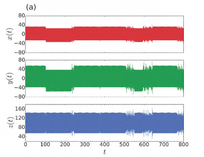
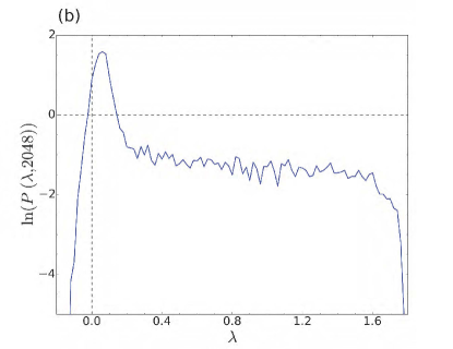
Figure 1: (Color online) (a) Time series showing intermittent chaos in the Lorenz system: $\dot{x}=a(y-x)$, $\dot{y}=x(r-z)-y$, $\dot{z}=xy-bz$, at parameter values $a=10$, $r=100.796$ and $b=8/3$. In this simulation a time step $\Delta t=1/64$ and initial condition (1,5,10) was used. (b) Logarithmic plot of the corresponding probability density, $P(\lambda,2048)$, for the distribution of ($10\,000$) maximal LLEs, $\lambda$, each obtained by averaging over $2048$ time steps. The bin width was set to $0.02$ and the total simulation time was $320\,000$.

shows the result of our calculations for the case of intermittent chaos in the well-known Lorenz system, as discussed in Ref. pra99 . As can be seen in Fig. 1(a), the time series for the system shows irregularly occurring bursts of almost periodic and chaotic behaviour. This motion corresponds to classic (Type-I) tangent bifurcation intermittency pom80 . In agreement with Fig. 6 of Ref. pra99 the characteristic distribution of LLEs consists of a superposition of two independent Gaussians, with stretched exponential interpolation between the two. Qualitatively, one can rationalize the shape of the distribution by considering that each Gaussian is roughly centered on the average value of the maximal LEs that would characterize each type of motion separately, i.e. if there was no switching.

Although the characteristic distributions of LLEs are stationary over a wide range of averaging times, the averaging time used to compute the LLEs does affect the widths of the distributions pra99 . Our numerical calculations confirm this observation. For very short averaging times the distributions are not stationary, i.e. they keep changing their shape, while in the asymptotic limit of infinite averaging times, they all tend towards delta functions. However, provided these two extremes are avoided, the distributions are stationary and maintain their characteristic shapes over a relatively wide range of averaging times.

We now turn our attention to computing the LLEs for chimera states. We begin by considering an interesting case of Eq. (1), that was analysed in detail by Wolfrum and Omel’chenko wol11a . The parameters $N$ and $R$ in Ref. wol11a correspond to $K=N/(2R)$,

$$C_{ij}=\left\{\begin{array}[]{ll}1&\mbox{if }|i-j|\leq R\mbox{ or }|i-j|\geq N-R\\ 0&\mbox{otherwise,}\end{array}\right.$$ (4)

and $G(x)=1$, in Eq. (1). In Fig. 2(a) we show the results of our simulation of this system after $400\,000$ time units. A snapshot of the distribution in phases, $\varphi_{i}$, and time averaged frequencies, $\left<\dot{\varphi}_{i}\right>$ (as well as the time series of the order parameter $Z(t)=\left|\sum_{k=1}^{N}\exp(i\varphi_{k})\right|$, not shown), clearly indicate that the oscillators are in a chimera state throughout the whole simulation. In Fig. 2(b) the corresponding distributions for the maximal LLE (blue, solid line) and all LLEs (red, dashed line), both averaged over $256$ time steps, can be seen.

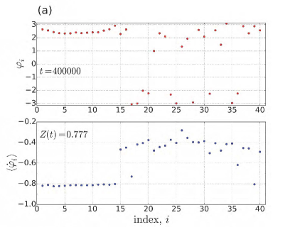
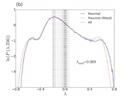
Figure 2: (Color online) (a) A snapshot of the phases $\varphi_{i}$ and time averaged frequencies $\left<\dot{\varphi}_{i}\right>$ for system (1) in a chimera state. Parameters: $N=40$, $R=14$, and $\alpha=1.478$. $\left<\dot{\varphi}_{i}\right>$ was averaged over $2048$ time steps, with $\Delta t=1/128$. (b) Corresponding probability distribution of the maximal LLEs (blue, solid line) and all LLEs (red, dashed line), averaged over $256$ time steps. The vertical dotted lines indicate the values of the LEs, the largest being $\lambda_{\rm max}\!=0.069$.

As observed in previous calculations of the LLEs pra99 , the distribution of all the exponents together has roughly the same shape as that of the maximal exponent alone. It is of course much smoother, due to the larger number of samples in the distribution, and is somewhat shifted towards the negative exponent side. The distribution shown in Fig. 2(b) appears to be characteristic to all chimera states arising from the general class of equations (1). It consists of a central asymmetric Gaussian-like peak with shoulders on both sides. One notable common feature in the distributions for chimera states is their approximate symmetry with respect to the $\lambda=0$ axis, c.f. the intermittent chaos distribution shown in Fig. 1(b). The feature of having two shoulders, one to either side of the main central peak, appears to be another distinguishing attribute specific to chimeras. To make these qualitative observations more precise we have fitted a variety of distributions corresponding to chimera states (all obtained from Eq. (1) at a variety of (very) different parameters) and found that all such distributions can be fitted accurately by a linear combination of four fitting functions (see Appendix B for details). By contrast, distributions of LLEs for intermittent chaos can be fitted to a comparable accuracy by a linear combination of only two Guassians and one exponential function.

Based on their analysis, Wolfrum and Omel’chenko wol11a have suggested that, “chimera states are chaotic transients”. Notwithstanding the experimental observations, there have been several counter-examples of numerically simulated chimera states that are stable, independent of the population size or initial conditions sch14 . In a general sense, the claim that chimera states are chaotic transients is therefore certainly not valid sud15 . Surprisingly, however, there have been very few comments about why this conclusion was reached for the prototype system pan15b . In the course of performing the present simulations, we have observed that the same system ($N=40$, $R=14$) is actually capable of supporting a variety of different chimera states, depending on the range of the “phase lag” parameter $\alpha$ pan13 ; abrphd . In our view the existence of chimera states in this system can be understood in terms of a balance between the tendency for the oscillators to synchronize, and the tendency for them not to. At the value $\alpha=1.46$, considered in Ref. wol11a , the overall coupling in the system was ‘attractive’, thus causing the system to synchronize after a certain time. The fact that the synchronization time was shown to be exponentially distributed (with respect to $N$) may be related to the probabilities of an individual oscillator to have an almost matching phase with one or more of its neighboring oscillators, i.e. as the system evolves. One can see this qualitatively from the equations of motion, by considering how $\alpha$ affects the slowing down or speeding up ($\dot{\varphi}$) of any individual oscillator due to its coupling with an equidistant pair of neighboring oscillators. To make these observations quantitative, is beyond the scope of the present work. For the system in Ref. wol11a it suffices to say that, depending on the value of $\alpha$, we have found that the initial chimera state may (i) synchronize completely after a certain time, (ii) persist (apparently) indefinitely, (iii) only appear intermittently between bursts of chaos, or (iv) collapse to an incoherent state after a very short time, never to re-appear again.

To investigate the effect of the above four scenarios on the distribution of LLEs, we have performed many simulations of the ($N=40$, $R=14$) system at different values of $\alpha$ in the range $[1.460,1.571]$. Each simulation had a slightly perturbed initial condition, as described in Ref. wol11a . The outcomes of our simulations all fall within the above categories: for $1.460\leqslant\alpha<1.513$, not all the initial chimera states persisted to the end of the simulation time ($400\,000$ time units). For $1.513\leqslant\alpha\leqslant 1.553$ all the chimera state persists throughout the whole simulation time. For $1.553<\alpha\leqslant 1.568$ chimera states appear intermittently, interrupted by bursts of chaos. Lastly, for $1.568<\alpha\leqslant 1.571$ the initial chimera rapidly evolved into permanent incoherence. In Fig. 3(a) we summarize these results by displaying time series of the order parameters at three different values of $\alpha$.

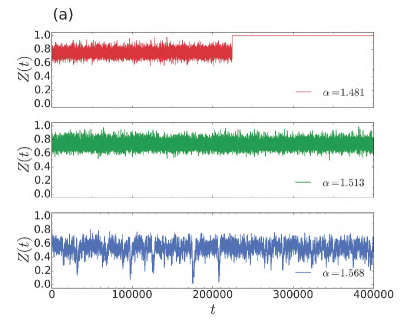
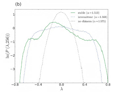
Figure 3: (Color online) (a) Time series of the order parameter $Z(t)=\left|\sum_{k=1}^{N}\exp(i\varphi_{k})\right|$ for three different types of chimera states. In the top figure ($\alpha=1.481$) the state is transient and the oscillators all synchronize for $t\gtrapprox 225\,000$ In the middle figure ($\alpha=1.513$) the state is stable, while in the bottom figure ($\alpha=1.568$) it appears intermittently. (b) The characteristic distributions of the maximal LLEs for stable and intermittent chimera states. For comparison the Gaussian distribution, expected for typical chaos (with no chimera), is also shown.

In the lower time series, for an intermittently occurring chimera at $\alpha=1.568$, two events can be seen where the order parameter drops down close to zero, i.e. intermittently the system becomes almost totally incoherent. For the majority of the simulation time $Z(t)$ hovers around $0.6$. Random spot checks on the phases and averaged frequencies show that the system is unambiguously in a chimera state for times when $Z(t)\gtrapprox 0.4$. Fig. 3(b) shows the corresponding distributions of the maximal LLEs corresponding to the cases (ii), (iii) and (iv), as described above. Here it can be seen that the characteristic distribution for the chimera state abruptly becomes flat-topped when the chimera starts to appear intermittently. Consistent with our expectations, once the chimera disappears completely the distribution corresponding to the incoherent oscillators is Gaussian in form. On the logarithmic plot that is shown in Fig. 3(b) it appears as a parabola, corresponding to the case of typical chaos.

We next consider the chimera state that was originally reported by Abrams and Strogatz abr04 for the system given by Eq. (1), or (2), with the coupling

$$G(x)=\frac{1}{2\pi}\left(1+0.995\cos x\right)\mbox{.}$$ (5)

As in Ref. abr04 , we solve this system for $N=K=256$ and $\alpha=\pi/2-0.18$, using Simpson’s $3/8$ rule jef08 , for which the quadrature weights in Eq. (1) are given by: $C_{k\,1}=3h/8$, $C_{k\,2}=9h/8$, $C_{k\,3}=9h/8$, $C_{k\,4}=6h/8$, $C_{k\,5}=9h/8$ , $C_{k\,6}=9h/8$, $C_{k\,7}=6h/8$, …, $C_{k\,N-1}=9h/8$, $C_{k\,N}=3h/8$. Here the space variable $x$ runs from $-\pi$ to $\pi$ with periodic boundary conditions, and $h=2\pi/N$ is the separation between the identical oscillators.

Fig. 4(a) shows the distribution of phases, averaged frequencies, and the time series of the order parameter for this chimera state. More importantly, Fig. 4(b) shows the distributions of all the LLEs, obtained by averaging over three different time intervals. As was previously mentioned, although all three distributions are stationary and maintain the shape of the characteristic distribution, their widths decrease as the averaging time increases from $128$ to $512$ time steps.

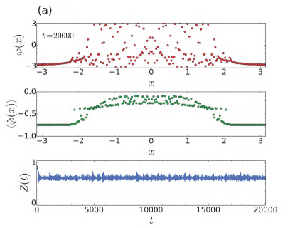
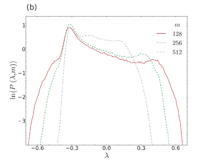
Figure 4: (Color online) (a) The chimera state for the system described in Ref. abr04 , showing a snapshot of the phases $\varphi(x)$ and time averaged phase velocities $\left<\dot{\varphi}(x)\right>$, after an integration time of $20000$ dimensionless units. The averaging for $\dot{\varphi}$ was done over $1024$ time steps, each of duration $\Delta t=1/128$. The lower figure shows the time series of the order parameter $Z(t)$. (b) Comparison of the characteristic distributions of all LLEs for the system in (a), obtained by averaging the LLEs over $128$, $256$ and $512$ time steps, respectively.

IV Conclusion

We have calculated the probability distributions of the local Lyapunov exponents (LLEs) corresponding to chimera states and found that they form a very characteristic distribution which appears to be specific to the state’s characteristic spatiotemporal pattern of synergistic coherent and incoherent motion. In principle a knowledge of this expected characteristic distribution can be used to identify the occurrence of chimera states in real physical systems, particularly in those for which it may not be possible to measure, directly the phases of of all the oscillators. In such cases, we envisage that advanced embedding techniques could be employed to extract the characteristic distribution of LLEs, which would then be a useful signature of the chimera state (for it would otherwise have been undetectable). The present results may thus find application in a variety systems where chimera states are relevant, but not necessarily directly observable. A comprehensive review of the relevant real-world systems may be found in Ref. pan15b and the references therein.

The case of intermittently appearing chimeras, as discussed in connection with Fig. 3, is currently of particular interest, in view of the fact that intermittent chaotic chimeras have only recently been reported in the literature for a much more complicated system olm15 . This system consisted of two symmetrically coupled populations of $N$ oscillators, where one population is synchronized and the other jumps erratically between laminar and turbulent phases olm15 . The present considerations indicate that such intermittency also arises in the original prototype system for chimera states, although it was not previously reported.

Appendix A Probability density of LLEs defined

Consider an autonomous $n$-dimensional continuous dynamical system of the form $\boldsymbol{\dot{x}}=F\left(\boldsymbol{x}\right)$. The probability density (distribution) of the $m$th LLE, $P\left(\lambda^{m},N\right)$, is defined so that $P\left(\lambda^{m},N\right)\mathrm{d}\lambda^{m}$ equals the probability that $\lambda_{N}^{m}$ takes on a value between $\lambda^{m}$ and $\lambda^{m}+\mathrm{d}\lambda^{m}$, where

$$\lambda_{N}^{m}=\frac{1}{N}\sum\limits_{j=1}^{N}\ln\left\|\boldsymbol{e}_{j}^{m}\right\|\mbox{.}$$ (6)

Here $\boldsymbol{e}_{0}^{m}$ is the $m$th vector of the initial set of orthonormal vectors, and $\boldsymbol{e}_{j}^{m}$ is its time evolved value under the action of the linearized equations of motion after $j$ time steps. Thus the $\boldsymbol{e}_{j}^{m}$ are obtained by solving the equations

$$\dot{\boldsymbol{e}}^{m}=\left\{\boldsymbol{J}F\left(\boldsymbol{x}\right)\right\}\boldsymbol{e}^{m}\mbox{,}$$ (7)

where $\boldsymbol{J}$ is the system Jacobian. Notice that $\lambda_{N}^{m}$ is the $m$th exponent averaged over $N$ time steps. Because the vectors $\boldsymbol{e}^{m}$ diverge exponentially in magnitude, and tend to align themselves along the local direction of most rapid growth, their exact directions may rapidly become numerically indistinguishable. To overcome this difficulty, as explained in Refs. shi79 ; ben80 ; wol85 , Gram-Schmidt orthogonalization can be performed on the set of frame vectors. In the present work we have performed the Gram-Schmidt orthogonalization after every time step.

Appendix B Fitting the characteristic distribution

It is found that the characteristic distribution of LLEs for chimera states can be fitted accurately by a linear combination of the form $g_{1}(x)+f(x)+g_{2}(x)+B\exp(-x/\tau)$, where $g_{1}$ and $g_{2}$ are Gaussians given by

$$g_{i}(x)=\frac{A_{i}}{\sigma_{i}\sqrt{2\pi}}\exp\left[-\left(\left(x-\mu_{i}\right)/\sqrt{2\sigma_{i}^{2}}\right)^{2}\right]\mbox{,}$$ (8)

and $f(x)$ is an exponentially modified Gaussian, given by

$$f(x)=\frac{A\gamma}{2}\exp\left(\frac{\mu-x+\gamma\sigma^{2}}{2/\gamma}\right)\mbox{erfc}\left(\frac{\mu+\gamma\sigma^{2}-x}{\sqrt{2\sigma^{2}}}\right)\mbox{,}$$ (9)

where erfc is the complementary error function jef08 . To perform the fitting we made use of the Python package lmfit new14 , which stands for Non-Linear Least-Squares Minimization and Curve-Fitting for Python. The initial parameters were chosen so that the Guassians were roughly centered on the two shoulders of the distribution, with $f(x)$ on the central main peak. In all cases, the distributions could be fitted with reduced chi-square values of less than 0.002.

For the data corresponding to the solid (blue) curve in Fig. 2(b), for example, the fitting routine produced the following output:

[[Model]]
    (((Model(gaussian, prefix=’g1_’)
     + Model(expgaussian, prefix=’f_’))
     + Model(gaussian, prefix=’g2_’))
     + Model(exponential, prefix=’exp_’))
[[Fit Statistics]]
    # function evals   = 970
    # data points      = 161
    # variables        = 12
    chi-square         = 0.088
    reduced chi-square = 0.001
[[Variables]]
    exp_amplitude:  -0.00123468 (init = 0.0)
    exp_decay:      -0.16029312 (init =-0.33)
    g1_sigma:        0.08416450 (init = 0.085)
    g1_center:      -0.53906326 (init =-0.54)
    g1_amplitude:    0.09116373 (init = 0.1)
    f_amplitude:     0.87642684 (init = 0.9)
    f_sigma:         0.09597549 (init = 0.09)
    f_center:       -0.29751003 (init =-0.3)
    f_gamma:         3.40994342 (init = 1)
    g2_sigma:        0.14054123 (init = 0.094)
    g2_center:       0.59176841 (init = 0.56)
    g2_amplitude:    0.09098822 (init = 0.054)

The fitted distribution has also been plotted in Fig. 2(b) as a dotted (black) line.

References

- (1) Ippei Shimada and Tomomasa Nagashima, “A numerical approach to ergodic problem of dissipative dynamical systems,” Prog. Theor. Phys. 61, 1605 (1979)
- (2) G. Benettin, L. Galgani, A. Giorgilli, and J.M. Strelcyn, “Lyapunov characteristic exponents for smooth dynamical systems and for Hamiltonian systems; a method for computing all of them,” Meccanica 15, 21 (1980)
- (3) A. Wolf, J. B. Swift, H. L. Swinney, and J. A. Vastano, “Determining Lyapunov exponents from a time series,” Physica D 16, 285 (1985)
- (4) P. Grassberger, R. Badii, and A. Politi, “Scaling laws for invariant measures on hyperbolic and nonhyperbolic atractors,” J. Stat. Phys. 51, 135–178 (1988)
- (5) Edward Ott, Chaos in Dynamical Systems (Cambridge University Press, Toronto, 1993)
- (6) T. Kapitaniak, “Distribution of transient Lyapunov exponents of quasiperiodically forced systems,” Prog. Theor. Phys. 93, 831–833 (1995)
- (7) E. J. Ding, “Characteristic distributions of finite-time lyapunov exponents,” Phys. Rev. E 60, 2761 (1999)
- (8) Arkady S. Pikovsky, “Local Lyapunov exponents for spatiotemporal chaos,” Chaos 3, 225–232 (1993)
- (9) O. Rudzick and A. Pikovsky, “Unidirectionally coupled map lattice as a model for open flow systems,” Phys. Rev. E 54, 5107 (1996)
- (10) G. Giacomelli, R. Hegger, A. Politi, and M. Vassalli, “Convective Lyapunov exponents and propagation of correlations,” Phys. Rev. Lett. 85, 3616 (2000)
- (11) C. Mendoza, S. Boccaletti, and A. Politi, “Convective instabilities of synchronization manifolds in spatially extended systems,” Phys. Rev. E 69, 047202 (2004)
- (12) Massimo Cencini and Alessandro Torcini, “Linear and nonlinear information flow in spatially extended systems,” Phys. Rev. E 63, 056201 (2001)
- (13) Bernhard Schmitzer, Wolfgang Kinzel, and Ido Kanter, “Pulses of chaos synchronization in coupled map chains with delayed transmission,” Phys. Rev. E 80, 047203 (2009)
- (14) Michael R. Allshouse and Thomas Peacock, “Refining finite-time Lyapunov exponent ridges and the challenges of classifying them,” Chaos 25, 087410 (2015)
- (15) K. Stefañski, K. Buszko, and K. Piecyk, “Transient chaos measurements using finite-time lyapunov exponents,” Chaos 20, 033117 (2010)
- (16) Daniel M. Abrams and Steven H. Strogatz, “Chimera states for coupled oscillators,” Phys. Rev. Lett. 93, 174102 (2004)
- (17) Y. Kuramoto and D. Battogtokh, “Coexistence of coherence and incoherence in nonlocally coupled phase oscillators,” Nonlinear Phenom. Complex Syst. 5, 380 (2002)
- (18) Daniel M. Abrams and Steven H. Strogatz, “Chimera states in a ring of nonlocally coupled oscillators,” Int. J. Bifurcation Chaos 16, 21 (2006)
- (19) Mark J. Panaggio and Daniel M. Abrams, “Chimera states on a flat torus,” Phys. Rev. Lett. 110, 094102 (2013)
- (20) Yusuke Suda and Koji Okuda, “Persistent chimera states in nonlocally coupled phase oscillators,” Phys. Rev. E 92, 060901(R) (2015)
- (21) Lennart Schmidt, Konrad Schönleber, Katharina Krischer, and Vladimir García-Morales, “Coexistence of synchrony and incoherence in oscillatory media under nonlinear global coupling,” Chaos 24, 013102 (2014)
- (22) Carlo R. Laing, “Chimeras in networks with purely local coupling,” Phys. Rev. E 92, 050904 (2015)
- (23) Matthias Wolfrum and Oleh E. Omel’chenko, “Chimera states are chaotic transients,” Phys. Rev. E 84, 015201(R) (2011)
- (24) M. Wolfrum, O. E. Omel’chenko, S. Yanchuk, and Y. L. Maistrenko, “Spectral properties of chimera states,” Chaos 21, 013112 (2011)
- (25) Daniel Michael Abrams, Two Coupled Oscillator Models: The Millennium Bridge and the Chimera State, Ph.D. thesis, Cornell University, Ithaca, New York (2006)
- (26) Aaron M. Hagerstrom, Thomas E. Murphy, Rojarshi Roy, Philipp Hoevel, Iryna Omelchenko, and Eckehard Schoell, “Experimental observation of chimeras in coupled-map lattices,” Nat. Phys. 8, 658 (2012)
- (27) Mark R. Tinsley, Simbarashe Nkomo, and Kenneth Showalter, “Chimera and phase-cluster states in populations of coupled chemical oscillators,” Nature Physics 8, 662 (2012)
- (28) Laurent Larger, Bogdan Penkovsky, and Yuri Maistrenko, “Virtual chimera states for delayed-feedback systems,” Phys. Rev. Lett. 111, 054103 (2013)
- (29) Erik Andreas Martens, Shashi Thutupalli, Antoine Fourrière, and Oskar Hallatscheka, “Chimera states in mechanical oscillator networks,” PNAS 110, 10563 (2013)
- (30) Tomasz Kapitaniak, Patrycja Kuzma, Jerzy Wojewoda, Krzysztof Czolczynski, and Yuri Maistrenko, “Imperfect chimera states for coupled pendula,” Scientific Reports 4, 6379 (2014)
- (31) Simona Olmi, Erik A. Martens, Shashi Thutupalli, and Alessandro Torcini, “Intermittent chaotic chimeras for coupled rotators,” Phys. Rev. E 92, 030901 (2015)
- (32) Mark J. Panaggio and Daniel M. Abrams, “Chimera states: Coexistence of coherence and incoherence in networks of coupled oscillators,” Nonlinearity 28, R67–R87 (2015)
- (33) Kurt Wiesenfeld and James W. Swift, “Averaged equations for Josephson junction series arrays,” Phys. Rev. E 51, 1020 (1995)
- (34) G. Filatrella, N. F. Pedersen, and K. Wiesenfeld, “Generalized coupling in the Kuramoto model,” Phys. Rev. E 75, 017201 (2007)
- (35) G. Filatrella, “Josephson junctions as a prototype for synchronization of nonlinear oscillators,” in New Developments in Josephson Junctions Research, edited by Sergei Sergeenkov (Transworld Research Network, Kerala, India, 2010) p. 83
- (36) N. Lazarides, G. Neofotistos, and G. P. Tsironis, “Chimeras in SQUID metamaterials,” Phys. Rev. B 91, 054303 (2015)
- (37) V. M. Bastidas, I Omelchenko, A. Zakharova, E. Schöll, and T. Brandes, “Quantum signatures of chimera states,” Phys. Rev. E 92, 062924(R) (2015)
- (38) R. Kleiner, F. Steinmeyer, G. Kunkel, and P. Muller, “Intrinsic Josephson effects in Bi2Sr2CaCu2O8 single crystals,” Phys. Rev. Lett. 68, 2394–2397 (1992)
- (39) Shi-Zeng Lin, “Mutual synchronization of two stacks of intrinsic Josephson junctions in cuprate superconductors,” J. Appl. Phys. 115, 173901 (2014)
- (40) D. A. Ryndyk, “Collective dynamics of intrinsic Josephson junctions in high- superconductors,” Phys. Rev. Lett. 80, 3376 (1998)
- (41) M. Machida, T. Koyama, and M. Tachiki, “Dynamical breaking of charge neutrality in intrinsic Josephson junctions: Common origin for microwave resonant absorptions and multiple-branch structures in the I-V characteristics,” Phys. Rev. Lett. 83, 4618 (1999)
- (42) Yu. M. Shukrinov, F. Mahfouzi, and N. F. Pedersen, “Investigation of the breakpoint region in stacks with a finite number of intrinsic Josephson junctions,” Phys. Rev. B 75, 104508 (2007)
- (43) E. M. Shahverdiev, L. H. Hashimova, P. A. Bayramov, and R. A. Nuriev, “Chaos synchronization between time delay coupled Josephson junctions governed by a central junction,” J. Supercond. Nov. Magn. 28, 3499–3505 (2015)
- (44) A. E. Botha, Yu. M. Shukrinov, S. Yu. Medvedeva, and M. R. Kolahchi, “Structured chaos in 1-d stacks of intrinsic Josephson junctions irradiated by electromagnetic waves,” J. Supercond. Novel Magnetism 28, 349–354 (2015)
- (45) A. E. Botha, Yu. M. Shukrinov, S. Emadi, and M. R. Kolahchi, “Chimeras states in coupled Josephson junctions,” Superconductor Science and Technology (communicated)(2016)
- (46) K. T. Alligood, T. D. Sauer, and J. A. Yorke, Chaos: An Introduction to Dynamical Systems (Springer-Verlag, New York, 1997)
- (47) R. C. Hilborn, Chaos and Nonlinear Dynamics: An Introduction, 2nd ed. (Oxford University Press, New York, 2000)
- (48) Toshiyuki Tanaka, Kazuyuki Aihara, and Masao Taki, “Lyapunov exponents of random time series,” Phys. Rev. E 54, 2122–2124 (1996)
- (49) Daniel J. Cross and R. Gilmore, “Differential embedding of the Lorenz attractor,” Phys. Rev. E 81, 066220 (2010)
- (50) Caixia Yang and Christine Qiong Wu, “A robust method on estimation of Lyapunov exponents from a noisy time series,” Nonlinear Dyn. 64, 279–292 (2011)
- (51) Caixia Yang, Christine Qiong Wu, and Pei Zhang, “Estimation of Lyapunov exponents from a time series for n-dimensional state space using nonlinear mapping,” Nonlinear Dyn. 69, 1493–1507 (2012)
- (52) Y. Kuramoto, Chemical Oscillations, Waves, and Turbulence, Chemistry Series (Dover, New York, 1984)
- (53) Oleh E. Omel’chenko, Yuri L. Maistrenko, and P. A. Tass, “Chimera states induced by spatially modulated delayed feedback,” Phys. Rev. E 82, 066201 (2010)
- (54) Iryna Omelchenko, Oleh E. Omel’chenko, Philipp Hövel, and Eckehard Schöll, “When nonlocal coupling between oscillators becomes stronger: Patched synchrony or multichimera states,” Phys. Rev. Lett. 110, 224101 (2013)
- (55) Gautam C. Sethia, Abhijit Sen, and George L. Johnston, “Amplitude-mediated chimera states,” Phys. Rev. E 88, 042917 (2013)
- (56) T. Bountis, V.G. Kanas, J. Hizanidis, and A. Bezerianos, “Chimera states in a two–population network of coupled pendulum–like elements,” Eur. Phys. J. Special Topics 223, 721–728 (2014)
- (57) R. Gopal, V. K. Chandrasekar, A. Venkatesan, and M. Lakshmanan, “Observation and characterization of chimera states in coupled dynamical systems with nonlocal coupling,” Phys. Rev. E 89, 052914 (2014)
- (58) Johanne Hizanidis, Vasileios G. Kanas, Anastasios Bezerianos, and Tassos Bountis, “Chimera states in networks of nonlocally coupled Hindmarsh-Rose neuron models,” Int. J. Bifurcation Chaos 24, 1450030 (2014)
- (59) Keren Li, Shen Ma, Haihong Li, and Junzhong Yang, “Transition to synchronization in a kuramoto model with the first- and second-order interaction terms,” Phys. Rev. E 89, 032917 (2014)
- (60) Gautam C. Sethia and Abhijit Sen, “Chimera states: The existence criteria revisited,” Phys. Rev. Lett. 112, 144101 (2014)
- (61) A. Zakharova, M. Kapeller, and E. Scholl, “Chimera death: Symmetry breaking in dynamical networks,” Phys. Rev. Lett. 112, 154101 (2014)
- (62) Mark J. Panaggio and Daniel M. Abrams, “Chimera states on the surface of a sphere,” Phys. Rev. E 91, 022909 (2015)
- (63) Bidhan Chandra Bag, K. G. Petrosyan, and Chin-Kun Hu, “Influence of noise on the synchronization of the stochastic Kuramoto model,” Phys. Rev. E 76, 056210 (2007)
- (64) Daniel M. Abrams, Rennie Mirollo, Steven H. Strogatz, and Daniel A. Wiley, “Solvable model for chimera states of coupled oscillators,” Phys. Rev. Lett. 101, 084103 (2008)
- (65) Daniel M. Abrams, Rennie Mirollo, Steven H. Strogatz, and Daniel A. Wiley, “Erratum: Solvable model for chimera states of coupled oscillators [phys. rev. lett. 101, 084103 (2008)],” Phys. Rev. Lett. 101, 129902 (2008)
- (66) Gautam C. Sethia, Abhijit Sen, and Fatihcan M. Atay, “Clustered chimera states in delay-coupled oscillator systems,” Phys. Rev. Lett. 100, 144102 (2008)
- (67) Ritwik K. Niyogi and L. Q. English, “Learning-rate-dependent clustering and self-development in a network of coupled phase oscillators,” Phys. Rev. E 80, 066213 (2009)
- (68) Carlo R. Laing, “The dynamics of chimera states in heterogeneous Kuramoto networks,” Physica D 238, 1569 (2009)
- (69) I. Martin, Gábor B. Halász, L. N. Bulaevskii, and A. E. Koshelev, “Shunt-capacitor-assisted synchronization of oscillations in intrinsic Josephson junctions stack,” J. Appl. Phys. 108, 033908 (2010)
- (70) Oleh E. Omel’chenko, Matthias Wolfrum, and Yuri L. Maistrenko, “Chimera states as chaotic spatiotemporal patterns,” Phys. Rev. E 81, 065201(R) (2010)
- (71) Hyunsuk Hong and Steven H. Strogatz, “Kuramoto model of coupled oscillators with positive and negative coupling parameters: An example of conformist and contrarian oscillators,” Phys. Rev. Lett. 106, 054102 (2011)
- (72) Oleh E. Omel’chenko, M. Wolfrum, S. Yanchuk, Y. L. Maistrenko, and O. Sudakov, “Stationary patterns of coherence and incoherence in two-dimensional arrays of non-locally-coupled phase oscillators,” Phys. Rev. E 85, 036210 (2012)
- (73) Y. Zhu, Y. Li, M. Zhang, and J. Yang, “The oscillating two-cluster chimera state in non-locally coupled phase oscillators,” Europhys. Lett. 97, 10009 (2012)
- (74) Oleh E. Omel’chenko, “Coherence-incoherence patterns in a ring of non-locally coupled phase oscillators,” Nonlinearity 26, 2469 (2013)
- (75) Nan Yao, Zi-Gang Huang, Ying-Cheng Lai, and Zhi-Gang Zheng, “Robustness of chimera states in complex dynamical systems,” Scientific Reports 3, 3522 (2013)
- (76) Jianbo Xie, Edgar Knobloch, and H-C Kao, “Multicluster and traveling chimera states in nonlocal phase-coupled oscillators,” Phys. Rev. E 90, 022919 (2014)
- (77) Jianbo Xie, H-C Kao, and Edgar Knobloch, “Chimera states in systems of nonlocal nonidentical phase-coupled oscillators,” Phys. Rev. E 91, 032918 (2015)
- (78) Y. Pomeau and P. Manneville, “Intermittent transition to turbulence in dissipative dynamical systems,” Commun. Math. Phys. 74, 189 (1980)
- (79) Alan Jeffrey and H.-H Dai, Handbook of Mathematical Formulas and Integrals, 4th ed. (Academic Press, Amsterdam, 2008)
- (80) Matthew Newville, Till Stensitzki, Daniel B. Allen, and Antonino Ingargiola, “LMFIT: Non-Linear Least-Square Minimization and Curve-Fitting for Python,” http://dx.doi.org/10.5281/zenodo.11813(2014)