Slow light in semiconductor quantum dots: effects of non-Markovianity and correlation of dephasing reservoirs

Abstract

A theoretical investigation on slow light propagation based on eletromagnetically induced transparency in a three-level quantum-dot system is performed including non-Markovian effects and correlated dephasing reservoirs. It is demonstraonated that the non-Markovian nature of the process is quite essential even for conventional dephasing typical of quantum dots leading to significant enhancement or inhibition of the group velocity slow-down factor as well as to the shifting and distortion of the transmission window. Furthermore, the correlation between dephasing reservoirs may also either enhance or inhibit non-Markovian effects.

I Introduction

Slow light group velocity propagation has revealed itself to be a key stone in the construction and design of variable delay lines which are of great importance in the synchronization of optical signals and signal buffering in all-optical communication systems. One of the most promising approaches is the one implementing electromagnetically induced transparency (EIT). eit_review It has been experimentally demonstrated that in EIT schemes it is possible to obtain a slow-down factor of $10^{7}$ in gases, such as Rb vapor gas and cold cloud of sodium atoms, sodium or solid-state systems as Pr doped solid Y₂SiO₅. However, the transmission bandwidths obtained in these systems are too narrow buffers (about 50-150 KHz) for optical buffers. Semiconductor structures such as quantum wells wells ; ultrawells and quantum dots cu ; kim ; peng ; mark ; bare may offer much broader transmission bandwidths (about a few GHz) at the cost of a smaller slow-down factor and with EIT buffers operating at room temperature. room ; su To open up possibilities in light control, one may combine EIT semiconductor structures with other systems capable of slowing light, i.e., photonic crystals lavr ; krauss ; baba or coupled quantum-dot heterostructures. braz

One feature of the semiconductor nanostructures such as quantum dots and wells is the interaction with the substrate host. For example, quantum dots interact with phonons or with carriers captured in traps in the vicinity of the quantum dot. The influence of the surroundings leads to dephasing and to energy loss of the semiconductor nanostructure. The most common dephasings and energy losses may be described by Markovian master equations usually written down in the so-called Lindblad form Lindblad (see, for example, the recent works by Colas et al Colas and Marques et al Marques ). Markovianity arises when correlations of dephasing or dissipative reservoirs rapidly decay on the typical time-scale of the nanostructure dynamics. However, it is well known that the dephasing process in solids is quite often of a non-Markovian nature as suggested in experimental dewoe and theoretical kilin studies. Reservoir correlations do not decay quickly enough and the density of reservoir states changes significantly on the scale of reservoir-system interaction constants and Rabi frequencies of driving fields. It is important to note that non-Markovian dephasing in quantum dots is responsible for phenomena such as, for instance, the damping of Rabi oscillations and excitation-induced dephasing, forstner ; our prl ; rams ; monni ; ulrich ; nazir ; hkim phonon-induced spectral asymmetry, hkim ; hug1 ; lodahl ; hug2 and interference between phononic and photonic reservoirs. calic ; vuk ; kau

To the best of our knowledge, only Markovian and uncorrelated dephasing have been considered in semiconductor EIT systems. In the present study, we show, for semiconductor quantum-dot systems, that the non-Markovian nature of dephasing leads to a significant modification of the group velocity slow-down factor in comparison with the Markovian one. Moreover, it is demonstrated that the absorption spectrum becomes asymmetric and the transmission window is shifted and modified. It is interesting that, in contrast with the damping of Rabi oscillations, forstner ; our prl ; rams ; monni the changes undergone by the slow-down factor and the transmission window are actually first-order effects on the frequency of the driving field associated with the Rabi oscillations. They may occur even in situations where the driving-induced dephasing and the damping of driven Rabi oscillations do not take place. Furthermore, correlations between dephasing reservoirs is also considered. Correlation between losses were already shown to lead to a number of non-trivial effects in the dynamics of open systems. ekert ; lidar ; valera ; our chain In this respect, well-known decoherence-free subspaces result from different couplings of the system with the same reservoir, and may be used for avoiding decoherence of the quantum states. ekert ; lidar Correlated losses may be exploited to create nonlinear loss in deterministic non-classical states generation valera and to produce excitation flow like heat while retaining coherence. our chain

The outline of the present study is as follows. In Section II we introduce the model of the three-level quantum dot in a ladder configuration under the action of both a strong pump and of a weak signal optical fields. The master equation and corresponding stationary solutions are presented in section III, whereas the susceptibility, absorption and slow-down factor are given in Section IV. In Section V, the influence of non-Markovian effects on the slow-down factor and absorption as well as some examples are analyzed. Also, a comparison with the Markovian case is demonstrated. Finally, discussion and conclusions are presented in Sections VI and VII, respectively.

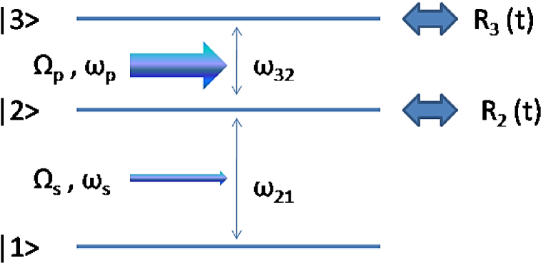
Figure 1: Pictorial view of a three-level quantum dot driven by a strong pump field with frequency $\omega_{p}$ and Rabi frequency $\Omega_{p}$. $R_{2}$ and $R_{3}$ denote dephasing reservoirs coupled to the corresponding levels described by states $|2\rangle$ and $|3\rangle$, respectively. The signal field with frequency $\omega_{s}$ and Rabi frequency $\Omega_{s}$. Dipole allowed transition frequencies are denoted by $\omega_{32}$ and $\omega_{21}$.

II The three-level quantum-dot model

The experimental setup needed to observe EIT involves two highly coherent optical fields interacting with a three level system in various schemes. Here, we are interested in a quantum dot model and therefore we choose a ladder scheme for EIT as depicted in Fig. 1: a weak signal field is tuned near resonance with the $|1\rangle\rightarrow|2\rangle$ transition, while a strong pump quasi-classical field is tuned with the $|2\rangle\rightarrow|3\rangle$ transition. We denote by $\omega_{s}$ and $\omega_{p}$ the optical frequencies of the signal and pump fields, respectively, and $\Omega_{s}$, $\Omega_{p}$ the Rabi frequencies associated with the signal and pump fields. Such a scheme was considered by Kim et al. kim for a strained GaAs-InGaAs-InAs quantum-dot system. We assume that $\omega_{21}$ and $\omega_{32}$ are sufficiently different so that the driving by the $\omega_{p}$ strong pump field (with $\Omega_{p}$ Rabi frequency) only occurs between upper states $|2\rangle$ and $|3\rangle$. Similarly, the $\omega_{s}$ weak signal field (with $\Omega_{s}$ Rabi frequency, $|\Omega_{s}|\ll|\Omega_{p}|$) acts only between states $|1\rangle$ and $|2\rangle$. Also, to illustrate the effects of the non-Markovian character of the dephasing process, we assume that energy loss occurs on times far exceeding the typical dephasing time of the quantum dot (e.g., in the study by Kim et al., kim for a GaAs-InGaAs-InAs quantum-dot system, dephasing times were about several tens of picoseconds at temperatures of 50 K - 80 K, whereas energy loss occurred on the scale of several nanoseconds). In the rotating-wave approximation and interaction representation, the three-level quantum dot scheme depicted in Fig. 1 may be described by the following generic Hamiltonian

$$V(t) = \hbar[\Delta_{s}+\Delta_{p}+R_{3}(t)]\sigma_{33}+\hbar[\Delta_{s}+R_{2}(t)]\sigma_{22}$$ (1)

$$+ \hbar\frac{\Omega_{p}}{2}(\sigma_{32}+\sigma_{23})+\hbar\frac{\Omega_{s}}{2}(\sigma_{21}+\sigma_{12}),$$

where, for simplicity, we assume $\Omega_{p}$ and $\Omega_{s}$ to be real, operators $\sigma_{kl}=|k\rangle\langle l|$ ($k,l=$1, 2, 3), $|k\rangle$ describes the $k$-th state of the system, and detunings are $\Delta_{s}=\omega_{21}-\omega_{s}$ and $\Delta_{p}=\omega_{32}-\omega_{p}$. The Hermitian operator $R_{k}=R_{k}(t)$ describes the dephasing reservoirs influencing the transition to the $k$-th state. We notice that one may exclude an action of a dephasing reservoir on the lower state by using $\sum\limits_{k=1}^{3}\sigma_{kk}=1$. Thus, each operator $R_{k}$ contains variables of two reservoirs (see, for example, the study by Kaer et al. lodahl ). Here we do not specify the exact nature of the dephasing reservoirs. It might include all types of pure dephasing encountered in quantum dots beyond the independent linear boson model commonly used to describe the phonon interaction with the dot, such as effects of possible quadratic coupling of phonons to the dot mul or phonon-phonon scattering. rudin We require only the existence of the quantities

$$D_{kl}^{\pm}(\delta)=\lim\limits_{t\rightarrow\infty}\int\limits_{0}^{t}d\tau K^{\pm}_{kl}(t,\tau)e^{i\delta\tau}$$ (2)

for any real $\delta$, where $K_{kl}^{+}(t,\tau)=\langle R_{k}(t)R_{l}(\tau)\rangle$ and $K_{kl}^{-}(t,\tau)=\langle R_{k}(\tau)R_{l}(t)\rangle$. For realistic many-system reservoirs one usually has $\langle R_{k}(x)R_{l}(y)\rangle\rightarrow 0$ for $|x-y|,\,x,\,y\rightarrow+\infty$ and the quantities (2) do exist, defining, for example, asymptotic decay rates obtained with the time-convolutioness master equation. BP

III The master equation

There is a strong pump field driving transition between states $|2\rangle$ and $|3\rangle$ of the three-level quantum dot. To derive a master equation accounting for effects of the strong dot-field interaction, it is necessary to transform to a dressed picture with respect to the operator

$$V_{d}=\hbar\Delta_{p}\sigma_{33}+\hbar\frac{\Omega_{p}}{2}(\sigma_{32}+\sigma_{23}).$$ (3)

The dressed Hamiltonian is

$$\mathbf{V}(t) = \hbar[\Delta_{s}+R_{3}(t)]{\bf S}_{33}(t)+\hbar[\Delta_{s}+R_{2}(t)]\mathbf{S}_{22}(t)$$ (4)

$$+ \hbar\frac{\Omega_{s}}{2}[\mathbf{S}_{21}(t)+\mathbf{S}_{12}(t)],$$

where the dressed operators are $\mathbf{S}_{kl}(t)=U^{\dagger}(t)\,\sigma_{kl}\,U(t)$, and $U(t)=\exp(-i\,V_{d}\,t/\hbar)$. Thus, for the population operators, one has our prl

$$\mathbf{S}_{33}(t) = S_{33}(t)\sigma_{33}+S_{23}(t)\sigma_{23}+S_{32}(t)\sigma_{32}$$ (5a)

$$+ S_{22}(t)\sigma_{22}$$

and

$$\mathbf{S}_{22}(t)=\sigma_{33}+\sigma_{22}-{\bf S}_{33}(t),$$ (5b)

where

$$S_{33}(t)=\frac{1}{2}\left[1+c^{2}+s^{2}\cos(\Omega_{R}t)\right],$$ (6a)

$$S_{22}(t)=\frac{s^{2}}{2}\left[1-\cos(\Omega_{R}t)\right],$$ (6b)

and

$$S_{23}(t)=\frac{s}{2}\left\{c[1-\cos(\Omega_{R}t)]+i\sin(\Omega_{R}t)\right\},$$ (6c)

with $\Omega_{R}^{2}=\Delta_{p}^{2}+\Omega_{p}^{2}$, $c=\Delta_{p}/\Omega_{R}$, $s=\Omega_{p}/\Omega_{R}$ and $S_{32}(t)=S_{23}^{*}(t)$.

Notice that here we assume low temperatures, so it is not necessary to consider multi-phonon processes and to implement polaron transformations to account for them. For low temperatures one may use the time-convolutioness master equation to describe the dynamics of the dot dressed by the driving field lodahl and derive in a standard manner the master equation for the ${\bar{\rho}}(t)$   dressed density matrix of the dot. BP Up to second order on the interaction involving reservoirs, one arrives at the following equation for the dressed density matrix averaged over the reservoirs

$$\frac{d}{dt}{\bar{\rho}}(t) = -i\left[\Delta_{s}\{\mathbf{S}_{22}(t)+\mathbf{S}_{33}(t)\},{\bar{\rho}}(t)\right]$$ (7)

$$+ i\left[\Omega_{s}\{\mathbf{S}_{21}(t)+\mathbf{S}_{12}(t)\},{\bar{\rho}}(t)\right]$$

$$- \int\limits_{0}^{t}d\tau\left\langle\left[V_{R}(t),\left[V_{R}(\tau),{\bar{\rho}}(t)\right]\right]\right\rangle,$$

where $V_{R}(t)=R_{3}(t)\mathbf{S}_{33}(t)+R_{2}(t)\mathbf{S}_{22}(t)$. Returning to the bare basis, one obtains the following equations for the off-diagonal (coherence) elements of the density matrix $\rho_{kl}=\langle k|\rho|l\rangle$,

$$\frac{d}{dt}\rho_{13}(t) = -[\gamma_{3}(t)-i(\Delta_{s}+\Delta_{p})]\rho_{13}(t)$$ (8a)

$$+ \left[\nu_{3}(t)-\frac{i}{2}\Omega_{p}\right]\rho_{12}(t)+\frac{i}{2}\Omega_{s}\rho_{23}(t),$$

and

$$\frac{d}{dt}\rho_{12}(t) = -[\gamma_{2}(t)-i\Delta_{s}]\rho_{12}(t)+\left[\nu_{2}(t)-\frac{i}{2}\Omega_{p}\right]\rho_{13}(t)$$ (8b)

$$+ \frac{i}{2}\Omega_{s}[\rho_{22}(t)-\rho_{11}(t)].$$

Notice that the form of the equations for coherences [Eqs. (8a) and (8b)] is the same for both Markovian and non-Markovian cases. However, a non-Markovian process leads to time-dependent coefficients in Eqs. (8) and also to their dependence on the driving field. The time-dependent decay rates in Eqs. (8) are $\gamma_{k}(t)=\gamma_{k}^{M}(t)+\gamma_{k}^{C}(t)$, where the $\gamma_{k}^{M}(t)$ represent decay rates for zero pump,

$$\gamma_{k}^{M}(t)=\int\limits_{0}^{t}d\tau K_{kk}^{-}(t,\tau),\quad k=2,\,3,$$ (9)

and the driving-dependent parts of the total decay rates are

$$\gamma_{2}^{C}(t)=\int\limits_{0}^{t}d\tau\,S_{22}(\tau-t)\left[K_{32}^{-}(t,\tau)-K_{22}^{-}(t,\tau)\right]$$ (10a)

and

$$\gamma_{3}^{C}(t)=\int\limits_{0}^{t}d\tau\,\left[1-S_{33}(\tau-t)\right]\left[K_{23}^{-}(t,\tau)-K_{33}^{-}(t,\tau)\right].$$ (10b)

The time-dependent cross-coherence coupling parameters in Eqs. (8) are

$$\nu_{2}(t)=\int\limits_{0}^{t}d\tau\,S_{32}(\tau-t)\left[K_{32}^{-}(t,\tau)-K_{22}^{-}(t,\tau)\right]$$ (11a)

and

$$\nu_{3}(t)=\int\limits_{0}^{t}d\tau\,S_{23}(\tau-t)\left[K_{33}^{-}(t,\tau)-K_{23}^{-}(t,\tau)\right].$$ (11b)

Notice that the decay rates introduced by Eqs. (9) and (10) might include imaginary components corresponding to driving-dependent frequency shifts. Eqs. (9), (10), and (11) give a clear idea about the influence of the reservoir correlation on the dynamics. Complete correlation between reservoirs, i.e., $K_{kl}^{-}(t,\tau)=K_{kl}^{+}(t,\tau)$, $k=2,\,3$, washes out the influence of an arbitrarily strong pump driving on the coherences dynamics. On the other hand, complete anti-correlation enhances the driving influence.

(a)

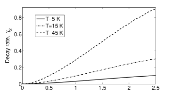
(b)

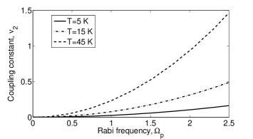
Figure 2: (a) $\gamma_{2}$ decay rate and (b) $\nu_{2}$ coupling constant as functions of the Rabi frequency $\Omega_{p}$, according to the reservoir correlation function given by Eq. (26). All quantities are defined in units of the typical Rabi frequency $\Omega_{0}=6.6$ $\mu$eV. kim Solid, dash-dotted and dotted lines correspond to temperatures $T=$5 K, 15 K, and 45 K, respectively.

(a)

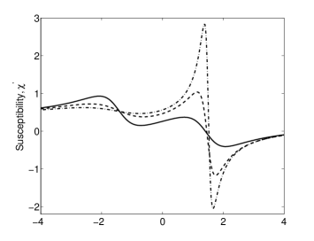
(b)

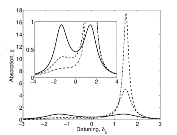
Figure 3: (a) Normalized linear susceptibility and (b) absorption profile in the weak non-Markovian case assuming $\gamma_{2}$ and $\gamma_{3}$ independent of $\Omega_{p}$ and $\nu_{2}\approx f_{2}\,\Omega_{p}$ [cf. Eq. (29) with $g_{2}=g_{3}=0$]. Here we take $\gamma_{3}=2\,\gamma_{2}=2\,\Omega_{0}$, $\nu_{3}=2\,\nu_{2}$, $\delta_{p}=0$, and $\Omega_{p}=3\,\Omega_{0}$. All parameters are given in units of $\Omega_{0}=6.6$ $\mu$eV. Solid, dashed and dash-dotted lines correspond to $f_{2}=0$ Markovian case, $f_{2}=0.1$ $\Omega_{0}$, and $f_{2}=0.2$ $\Omega_{0}$, respectively. Other parameters are the same as in the study by Kim et al. kim : $\varepsilon_{bac}=13$, $|\mu_{21}|/e=2.1$ nm, $\Gamma=0.006$, $V=8.9064\times 10^{2}$ nm³, and the wavelength of the signal field is 1.36 $\mu$m. Inset in panel (b) shows the absorption profiles in more detail.

Figure 4: Slow-down factor [cf. Eq.(16)] in the weak non-Markovian case assuming $\nu_{2}\approx f_{2}\,\Omega_{p}$ [$g_{2}=g_{3}=0$ in Eq. (29)] and $\delta_{p}=\delta_{s}=0$. Solid, dashed and dash-dotted lines correspond to the $f_{2}=0$ Markovian case, $f_{2}=0.1$ $\Omega_{0}$, and $f_{2}=0.2$ $\Omega_{0}$, respectively. The other parameters are chosen as in Fig. 3.

IV Susceptibility, absorption and slow-down factor

Now let us consider the solution of the system of Eqs. (8) in the $t\rightarrow\infty$ limit. We assume that $\lim\limits_{t\rightarrow\infty}\rho_{kl}(t)\equiv\rho_{kl}^{st}$, $\lim\limits_{t\rightarrow\infty}\nu_{k}(t)\equiv\nu_{k}$, and introduce real asymptotic values of the dephasing rates

$$\gamma_{k}=\mathrm{Re}\left[\lim\limits_{t\rightarrow\infty}\gamma_{k}(t)\right],$$ (12)

and modified detunings

$$\delta_{s}=\Delta_{s}+\mathrm{Im}\left[\lim\limits_{t\rightarrow\infty}\gamma_{2}(t)\right]$$ (13a)

and

$$\delta_{p}=\Delta_{p}+\mathrm{Im}\left[\lim\limits_{t\rightarrow\infty}\gamma_{3}(t)\right].$$ (13b)

The stationary solutions for the coherence are then given by

$$\rho_{13}^{st}=\frac{(2\nu_{3}-i\Omega_{p})\rho_{12}^{st}-i\Omega_{s}\rho_{23}^{st}}{2[\gamma_{3}-i(\delta_{s}+\delta_{p})]}$$ (14a)

and

$$\rho_{12}^{st}=\frac{(2\nu_{2}-i\Omega_{p})\rho_{13}^{st}-i\Omega_{s}(\rho_{22}^{st}-\rho_{11}^{st})}{2(\gamma_{2}-i\delta_{s})}.$$ (14b)

Taking into account that the pump driving field is much more intense than the signal field ($|\Omega_{p}|\gg|\Omega_{s}|$), one obtains kim for the $\chi^{{}^{\prime}}$ linear susceptibility and $\chi^{{}^{\prime\prime}}$ absorption rate houm

$$\chi^{{}^{\prime}} \approx \varepsilon_{bac}+\frac{\Phi}{\hbar\Xi}\,\gamma_{3}\left(\gamma_{3}\delta_{s}+\Omega_{p}\frac{\nu_{2}+\nu_{3}}{2}\right)$$ (15a)

$$+ \frac{\Phi}{\hbar\Xi}(\delta_{p}+\delta_{s})\left(\nu_{2}\nu_{3}-\frac{\Omega^{2}_{p}}{4}+(\delta_{s}+\delta_{p})\delta_{s}\right)$$

and

$$\chi^{{}^{\prime\prime}}\approx\frac{\Phi}{\hbar\Xi}\gamma_{3}\left(\gamma_{3}\gamma_{2}+\frac{\Omega^{2}_{p}}{4}\right)+\frac{\Phi}{\hbar\Xi}\left[\gamma_{2}(\delta_{s}+\delta_{p})^{2}-\gamma_{3}\nu_{2}\nu_{3}\right],$$ (15b)

where $\Xi=[\gamma_{3}\gamma_{2}+\Omega^{2}_{p}/4-\nu_{2}\nu_{3}-(\delta_{s}+\delta_{p})\delta_{s}]^{2}+[\gamma_{2}(\delta_{s}+\delta_{p})+\gamma_{3}\delta_{s}+\Omega_{p}(\nu_{2}+\nu_{3})/2]^{2}$, $\Phi=\Gamma|\mu_{12}|^{2}(\rho_{11}^{st}-\rho_{22}^{st})/\epsilon_{0}\Theta$, $\varepsilon_{bac}$ is the background dielectric constant, $\mu_{12}$ is the dipole moment of the transition between states $|1\rangle$ and $|2\rangle$, $\epsilon_{0}$ is the vacuum electric permittivity, and $\Theta$ is the volume of a single quantum dot. $\Gamma$ is the optical confinement factor defined as the fraction of the field intensity confined to the dots. and Here we assume that our structure is typical for vertical-cavity quantum dot lasers, where light propagates perpendicular to the active layer. Thus,

$$\Gamma\approx\zeta\frac{\int\limits_{dot}dzI(z)}{\int\limits_{structure}dzI(z)},$$

$I(z)$ being the field intensity as a function of the coordinate along the direction of propagation and $\zeta$ is the ratio of the dots area to the area of the structure in the direction perpendicular to the signal-field propagation. Roughly, $\Gamma$ is proportional to the ratio of the total dot volume to the volume of the structure. Here we assume that the dot remains on the lower $|1\rangle$ state, so that $\rho_{22}^{st}\ll\rho_{11}^{st}\approx 1$. The slow-down factor, defined as the ratio of the group velocities of light outside and inside the slowing medium, is given in our case by

$$\Upsilon=n+\omega_{s}\frac{dn}{d\omega_{s}},$$ (16)

where $n=\sqrt{\chi^{{}^{\prime}}+i\chi^{{}^{\prime\prime}}}$ is the complex refractive index.

(a)

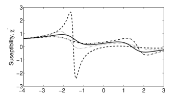
(b)

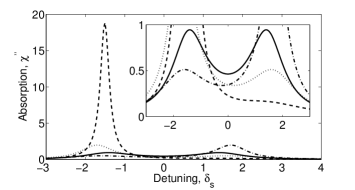
Figure 5: (a) Normalized linear susceptibility and (b) absorption profile in the weak non-Markovian case assuming $\nu_{2}\approx f_{2}\,\Omega_{p}$ [$g_{2}=g_{3}=0$ in Eq. (29)]. Solid, dashed, dash-dotted and dotted lines correspond to the $(f_{2},f_{3})=(0,0)$ Markovian case, $(f_{2},f_{3})=(-0.2,-0.4)\,\Omega_{0}$, $(f_{2},f_{3})=(-0.2,0.4)\,\Omega_{0}$, and $(f_{2},f_{3})=(0.2,-0.4)\,\Omega_{0}$, respectively. Other parameters are chosen as in Fig. 3. Inset in panel (b) shows the absorption profiles in more detail.

V Non-Markovian effects

Let us consider the asymptotic values of $\gamma_{k}$ and $\nu_{k}$ to establish the non-Markovian dynamics of the system. One then obtains

$$\gamma_{2} = D^{-}_{22}(0)+\frac{s^{2}}{2}[D^{-}_{32}(0)-D^{-}_{22}(0)]-\frac{s^{2}}{4}\left[D^{-}_{32}(\Omega_{R})\right.$$ (17)

$$- D^{-}_{22}(\Omega_{R})+\left.D^{-}_{32}(-\Omega_{R})-D^{-}_{22}(-\Omega_{R})\right]$$

and

$$\gamma_{3} = D^{-}_{33}(0)+\frac{s^{2}}{2}[D^{-}_{23}(0)-D^{-}_{33}(0)]-\frac{s^{2}}{4}\left[D^{-}_{23}(\Omega_{R})\right.$$ (18)

$$- \left.D^{-}_{33}(\Omega_{R})+D^{-}_{23}(-\Omega_{R})-D^{-}_{33}(-\Omega_{R})\right].$$

The $t\rightarrow\infty$ limit is equivalent to the Markovian approximation. We note that, due to the driving field, $\gamma_{k}$ and $\nu_{k}$ are dependent on the values of the Fourier-transforms [cf. Eq. (2)] of the reservoir correlation functions at $\delta=0,\,\pm\,\Omega_{R}$ (hence the name local Markovian approximation john ), whereas for the traditional Markovian approximation the rates are only dependent on the value of the Fourier-transforms at $\delta=0$. We assume weak non-Markovian effects, i.e., if $D_{kl}^{-}(\omega)$ is smooth in the vicinity of $\omega=0$ and varies only slightly on the scale defined by the modified Rabi frequency $\Omega_{R}$, then it may be represented as a polynomial up to second order in $\omega$. Therefore, Eq. (17) reduces to

$$\gamma_{2}\approx\left.D^{-}_{22}(0)-\frac{\Omega_{p}^{2}}{4}\frac{d^{2}}{d\omega^{2}}\left[D^{-}_{32}(\omega)-D^{-}_{22}(\omega)\right]\right|_{\omega\rightarrow 0}.$$ (19)

Similarly, one obtains for the $\gamma_{3}$ decay rate

$$\gamma_{3}\approx\left.D^{-}_{33}(0)-\frac{\Omega_{p}^{2}}{4}\frac{d^{2}}{d\omega^{2}}\left[D^{-}_{23}(\omega)-D^{-}_{33}(\omega)\right]\right|_{\omega\rightarrow 0}.$$ (20)

Therefore, the decay rates depend on the squared Rabi frequency associated with the driving field. Here we note that such a dependence leads to the damping of the driven Rabi oscillations. our prl Similarly, for the coupling parameters from Eq. (2) one obtains

$$\nu_{2} = \frac{sc}{2}\left[D^{-}_{32}(0)-D^{-}_{22}(0)\right]-\frac{s}{4}(1+c)\left[D^{-}_{32}(\Omega_{R})\right.$$ (21)

$$- \left.D^{-}_{22}(\Omega_{R})\right]+\frac{s}{4}(1-c)\left[D^{-}_{32}(-\Omega_{R})\right.$$

$$- \left.D^{-}_{22}(-\Omega_{R})\right]$$

and

$$\nu_{3} = \frac{sc}{2}[D^{-}_{33}(0)-D^{-}_{23}(0)]+\frac{s}{4}(1-c)\left[D^{-}_{33}(\Omega_{R})\right.$$ (22)

$$- \left.D^{-}_{23}(\Omega_{R})\right]-\frac{s}{4}(1+c)\left[D^{-}_{33}(-\Omega_{R})\right.$$

$$- \left.D^{-}_{32}(-\Omega_{R})\right].$$

As before, it is straightforward to show that Eqs. (21) and (22) lead to

$$\nu_{2} \approx \left.\frac{\Omega_{p}}{2}\frac{d}{d\omega}\left[D^{-}_{22}(\omega)-D^{-}_{32}(\omega)\right]\right|_{\omega\rightarrow 0}$$ (23)

$$+ \left.\frac{\Omega_{p}\Delta_{p}}{2}\frac{d^{2}}{d\omega^{2}}\left[D^{-}_{22}(\omega)-D^{-}_{32}(\omega)\right]\right|_{\omega\rightarrow 0}$$

and

$$\nu_{3} \approx \left.\frac{\Omega_{p}}{2}\frac{d}{d\omega}\left[D^{-}_{33}(\omega)-D^{-}_{23}(\omega)\right]\right|_{\omega\rightarrow 0}$$ (24)

$$+ \left.\frac{\Omega_{p}\Delta_{p}}{2}\frac{d^{2}}{d\omega^{2}}\left[D^{-}_{33}(\omega)-D^{-}_{23}(\omega)\right]\right|_{\omega\rightarrow 0}.$$

One may note that, for the calculation of the coherence coupling parameters, it is sufficient for the transforms of the $D_{kl}^{-}(\omega)$ bath correlation functions to be linearly dependent on the frequency to have the non-Markovianity affecting the susceptibility and absorption. As we shall see below, even for $|D_{kl}^{-}(\Omega_{R})-D_{kl}^{-}(0)|\ll|\Omega_{R}|$, the influence of non-Markovianity on the susceptibility, absorption and the slow-down factor may be quite pronounced.

To demonstrate that it is quite common that non-Markovianity leads to significant coherence coupling parameters, let us consider a model of pure dephasing produced by the reservoir of acoustic phonons at low but finite temperature. Such a model has been extensively used for describing pure dephasing. forstner ; rams ; monni ; ulrich ; nazir ; hkim ; hug1 ; lodahl ; hug2 ; calic ; vuk In the interaction picture with respect to the phonon reservoir, the reservoir operators are described by BP

$$R_{k}(t)=\sum\limits_{l}g_{kl}\left(b_{l}e^{-iw_{l}t}+b_{l}^{\dagger}e^{iw_{l}t}\right),$$ (25)

where the $b_{l}$ and $b_{l}^{\dagger}$ are annihilation and creation operators of the phonon mode with frequency $w_{l}$ and the $g_{lk}$ are interaction constants (for simplicity, assumed as real).

As an example, let us take just one correlation function [i.e., $K_{22}(\tau,t)$] assuming there is no correlation between reservoirs. For the reservoir at temperature $T$,

$$K_{22}(\tau,t)=\sum\limits_{l}g_{2l}^{2}\left[\left[n_{T}(w_{l})+1\right]e^{-iw_{l}(\tau-t)}+n_{T}(w_{l})e^{iw_{l}(\tau-t)}\right]=\int\limits_{0}^{\infty}dwJ(w)\left[\left[n_{T}(w)+1\right]e^{-iw_{l}(\tau-t)}+n_{T}(w)e^{iw_{l}(\tau-t)}\right],$$ (26)

where the average number of thermal phonons in the mode is

$$n_{T}(w)=\coth\left(\frac{\hbar w}{2k_{B}T}\right)$$ (27)

and the function $J(w)$ is the density of states of the phonon reservoir. Let us consider a typical super-Ohmic density of states

$$J(w)=\alpha w^{3}\exp\left[-\frac{w^{2}}{2w_{c}^{2}}\right],$$ (28)

where $\alpha$ accounts for the interaction strength and $w_{c}$ is the cut-off frequency. Such a function describes a reservoir of acoustic phonons identified, for example, as a major source of pure dephasing in InGaAs/GaAs quantum dots. rams We take $\alpha=0.4\pi^{2}$ ps^-2 (see, for example, Hughes et al. hug2 ) and assume a cut-off frequency $w_{c}=1$ meV. Fig. 2 displays the dependence of the $\gamma_{2}$ driving-dependent decay rate [see Eq. (17)] and $\nu_{2}$ coupling constant [cf. Eq. (21)] on the $\Omega_{p}$ Rabi frequency. We have scaled all the quantities with the typical value kim of the Rabi frequency of the driving field, $\Omega_{0}=6.6$ $\mu$eV. One may see that, for low temperatures (5 K-45 K was used for simulations in Fig. 2), the dependence of decoherence rates and coupling constants on the driving field is indeed quite pronounced and, quite definitely, may not be ignored.

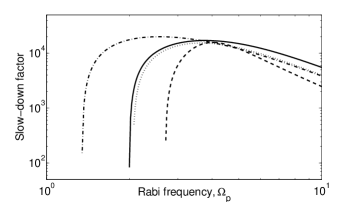
Figure 6: Slow-down factor [cf. Eq.(16)] in the weak non-Markovian case assuming $\nu_{2}\approx f_{2}\,\Omega_{p}$ [cf. Eq. (29) with $g_{2}=g_{3}=0$] and $\delta_{p}=\delta_{s}=0$. Solid, dashed, dash-dotted and dotted lines correspond to the $(f_{2},f_{3})=(0,0)$ Markovian case, $(f_{2},f_{3})=(-0.2,-0.4)\,\Omega_{0}$, $(f_{2},f_{3})=(-0.2,0.4)\,\Omega_{0}$, and $(f_{2},f_{3})=(0.2,-0.4)\,\Omega_{0}$, respectively. Other parameters are chosen as in Fig. 3.

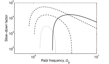
Figure 7: Slow-down factor in the weak non-Markovian case. Here [cf. Eq. (29)] $f_{3}=2\,f_{2}$, $g_{3}=2\,g_{2}$, $\delta_{p}=\delta_{s}=0$. Solid, dashed, dash-dotted and dotted lines correspond to the $(f_{2},g_{2})=(0,0)$ Markovian case, $(f_{2},g_{2})=(0.2,0.0001)\,\Omega_{0}$, $(f_{2},g_{2})=(0.2,0.1)\,\Omega_{0}$, and $(f_{2},g_{2})=(0.2,0.15)\,\Omega_{0}$, respectively. Other parameters are chosen as in Fig. 3.

VI Discussion and Examples

Here we wish to investigate the influence of non-Markovian effects on the susceptibility and absorption of a three-level quantum dot. To this end, we compare the Markovian and non-Markovian regimes and analyze the influence of non-Markovian effects and correlated dephasing reservoirs.

In the Markovian limit we choose the values of parameters used by Kim et al. kim in the case of a cylindrical strained GaAs-InGaAs-InAs quantum-dot system, i.e., $\varepsilon_{bac}=13$, $|\mu_{21}|/e=2.1$ nm, $\Gamma=0.006$, $V=8.9064\times 10^{2}$ nm³, and the wavelength of the signal field is 1.36 $\mu$m, which is much shorter than the wavelength of the driving field (12.8 $\mu$m). Also, it was assumed that the dephasing rate for level 3 was two times larger than for level 2. In the results shown below we also make this assumption for both the dephasing rates and coupling parameters $\gamma_{3}=2\gamma_{2}$ and $|\nu_{3}|=2|\nu_{2}|$. Moreover, here we assume that decay rates and coupling constants depend on the Rabi frequency associated with the driving field [cf. Eqs. (19)-(20) and (23)-(24)] as

$$\gamma_{k}\approx\gamma_{k}^{(0)}+\frac{g_{k}}{2}\Omega_{p}^{2},\quad\nu_{k}\approx f_{k}\Omega_{p}+g_{k}\Delta_{p}\Omega_{p},$$ (29)

for $k=2,\,3$. As mentioned, $D_{kk}^{-}$ has been represented as a polynomial up to second order in $\omega$, i.e., $D_{kk}^{-}(\omega)\approx\gamma^{(0)}_{k}+2f_{k}\,\omega+g_{k}\,\omega^{2}$ for $k=2,\,3$. In addition, $D_{32}^{-}(\omega)=D_{23}^{-}(\omega)=0$. It should be noted here that $\gamma_{k}^{(0)}$ rates might also include a contribution from Markovian reservoirs describing energy loss and other sources of Markovian dephasing. Let us first consider the case of a negligible change of the decay rate with the Rabi frequency, i.e., $\gamma_{k}^{(0)}\gg|\frac{g_{k}}{2}\Omega_{p}^{2}|$ for $k=2,\,3$. Weak non-Markovian effects ($|f_{k}\Omega_{p}|\ll\gamma_{k}^{(0)}$, $k=2,\,3$) on the susceptibility, absorption and slow-down factor, are then illustrated in Figs. 3 and 4. Fig. 3(a) depicts the susceptibility for the Markovian resonant ($f_{2}=0$, $\Delta_{p}=0$) and two non-Markovian cases ($f_{2}=0.1\,\Omega_{0}$, $f_{2}=0.2\,\Omega_{0}$, $\Delta_{p}=0$) as a function of the signal-field $\delta_{s}$ detuning. One notices that the slope of the non-Markovian susceptibility curve is indeed rather pronouncedly enhanced. In addition, as indicated by results from the absorption profiles in Fig. 3(b), non-Markovian effects shift and narrow the transmission bandwidths (the latter is natural to expect; see, for example, Tucker et al. buffers ). Moreover, the increase in the slow-down factor may be quite large (cf. Fig. 4) whereas the transmission bandwidth is not significantly reduced. Non-Markovian effects are phase-sensitive and may be either harmful or advantageous for slowing down light. Simultaneous changes of sign of coupling constants $\nu_{2}$ and $\nu_{3}$ shift the peaks of both the susceptibility and absorption to the region of negative $\delta_{s}$ detunings (see Figs. 5 and 6). However, the change is not completely symmetrical and gain in the slow-down factor is smaller than in the case of $\nu_{2}$ and $\nu_{3}$ both positive. It is interesting to point out that taking $\nu_{2}$ and $\nu_{3}$ of opposite signs, one may simultaneously obtain both the enhancement of the slow-down factor and widening of transmission bandwidth [see inset in Fig. 5(b) and Fig. 6].

Up to now we have considered decay rates independent of the Rabi frequency $\Omega_{p}$. As we have shown before, such dependencies may be considered through Eq. (29) by taken $g_{k}\neq 0$ ($k=2,\,3$). In this case, the non-Markovian nature of the EIT process may destroy the efficiency in obtaining slow light. To see this, we turn to Fig. 7 where the behavior of the slow-down factor is plotted as a function of the Rabi frequency associated with the pump field. If decay rates depend on the Rabi frequency $\Omega_{p}$, one may obtain EIT systems with worse performance than in the Markovian case. As such dependence becomes more remarkable, i.e, as $g_{2}$ and $g_{3}$ are increased [cf. Eq. (29)], a shifting and narrowing of the transmission window is more noticeable, and a complete loss of the non-Markovian slow-down effect may be obtained as the Rabi frequency $\Omega_{p}$ is increased.

We note that correlations between reservoirs may affect the influence of memory effects on the slow-down factor. In a quantum dot system, the interaction between the dot electrons and its surrounding medium, i.e., impurities, phonons, etc., may lead to significant correlations between reservoirs. Moreover, by construction, operators $R_{k}(t)$ ($k=2,\,3$) contain variables corresponding to the same reservoir acting on the lower level of the dot. To see how the correlation between reservoirs is inevitably arising in conventional models of dephasing, let us consider an example of the electron-phonon interaction constants [cf. Eq. (25)] for the present three-level dot. They may be represented in the following general form hug1

$$g_{kl}=C\sqrt{\hbar|\mbox{$\vec{\mathbf{L}}$}|}\int d^{3}\mbox{$\vec{\mathbf{r}}$}\left[d_{k}|\phi_{k}(\mbox{$\vec{\mathbf{r}}$})|^{2}-d_{1}|\phi_{1}(\mbox{$\vec{\mathbf{r}}$})|^{2}\right]e^{i\mbox{$\vec{\mathbf{L}}$}\cdot\mbox{$\vec{\mathbf{r}}$}},$$ (30)

where $\vec{\mathbf{L}}$ is the wave-vector of the $l$-th phonon mode, $d_{k}$ and $\phi_{k}(\mbox{$\vec{\mathbf{r}}$})$ are the deformation potential and the electron wave-function of the $k$-th state of the dot, respectively, and $C$ is a constant. Since electron wave-functions are localized in the vicinity of the dot, and taking into account the small energies of acoustic phonons (in the present case it would be much less than 1 meV), the densities of states of the phononic reservoirs corresponding to states $|2\rangle$ and $|3\rangle$ should be similar. The difference in the integrand of Eq. (30) involves essentially the values of the $d_{k}$ deformation potential. If the deformation potentials are close in values for different excited states, the model defined in Eq. (25) predicts obliteration of the non-Markovian effect by correlated dephasing. Notice that, for an adequate treatment of correlations between reservoirs, one needs to appropriately account for phase differences between constants $g_{kl}$ to develop a realistic microscopic dephasing model.

VII Conclusions

In conclusion, we have shown that it is necessary to take into account non-Markovian effects when considering slowing down light in EIT schemes based on quantum dots. Non-Markovian behavior is typical for such systems, especially in low temperature conditions. We have demonstrated that, for decay rates independent of the Rabi frequency associated with the pump field, even relatively weak non-Markovian effects may lead to significant enhancement of the slow-down factor together with the simultaneous broadening of the transmission window. However, if decay rates are considered to be dependent of the Rabi frequency $\Omega_{p}$, a shifting and narrowing of the transmission window may be obtained. Furthermore, non-Markovian effects may lead to significant driving-induced dephasing which may inhibit the slowing-down effect. Moreover, it is suggested that the presence of correlation between reservoirs may remove the harmful effects produced by the non-Markovian nature of EIT. Finally, considering the importance of investigations to produce efficient slow light propagation in solid-state systems, we do hope this work would stimulate future experimental and theoretical studies on this subject.

- (1) M. Fleischhauer, A. Imamoglu, and J. P.Marangos, Rev. Mod. Phys. 77, 633 (2005).
- (2) D. F. Phillips, A. Fleischhauer, A. Mair, R. L. Walsworth, and M. D. Lukin, Phys. Rev. Lett. 86, 783 (2001).
- (3) C. Liu, Z. Dutton, C. Behroozi, and L. V. Hau, Nature 409, 490 (2001).
- (4) A. V. Turukhin, V. S. Sudarshanam, M. S. Shahriar, J. A. Musser, B. S. Ham, and P. R. Hemmer, Phys. Rev. Lett. 88, 023602 (2002).
- (5) R. S. Tucker, Pei-Cheng Ku, and C. J. Chang-Hasnain, J. Lightwave Tech. 23, 4046 (2005).
- (6) Pei-Cheng Ku, F. Sedgwick, C. J. Chang-Hasnain, Ph. Palinginis, T. Li, H. Wang, Shu-Wei Chang, and Shun-Lien Chuang, Opt. Lett. 29, 2291 (2004).
- (7) P. Palinginis, S. Crankshaw, F. Sedgwick, E.-T. Kim, M. Moewe, C. J. Chang-Hasnain, H. Wang, and S. L. Chuang, Appl. Phys. Lett. 87, 171102 (2005).
- (8) Pei Cheng Ku, C. J. Chang-Hasnain, and S. L. Chuang, Electr. Lett. 38, 1581 (2002).
- (9) J. Kim, S. I. Chuang, P. C. Ku, and C. J. Chuang-Hasnain, J. Phys.: Cond. Matter 16, S3727 (2004).
- (10) P. C. Peng, H. C. Kuo, W. K. Tsai, Y. H. Chang, C. T. Lin, S. Chi, S. C. Wang, G. Lin, H. P. Yang, K. F. Lin, H. C. Yu, and J. Y. Chi, Opt. Express 14, 2944 (2006).
- (11) S. Marcinkevicius, A. Gushterov, and J. P. Reithmaier, Appl. Phys. Lett. 92, 041113 (2008).
- (12) D. Barettin, J. Houmark, B. Lassen, M. Willatzen, T. R. Nielsen, J. Mørk, and A.-P. Jauho, Phys. Rev. B 80, 235304 (2009).
- (13) P. Palinginis, F. Sedgwick, S. Crankshaw, M. Moewe, and C. Chang-Hasnain, Opt. Express 13, 9909 (2005).
- (14) H. Su and S. Chuang, Opt. Lett. 31, 271 (2006).
- (15) T. F. Krauss, Nature Photonics 2, 448 (2008).
- (16) T. Baba, Nature Photonics 2, 465 (2008).
- (17) T. R. Nielsen, A. Lavrinenko, and J. Mork, Appl. Phys. Lett. 94, 113111 (2009).
- (18) H. S. Borges, L. Sanz, J. M. Villas-Boas, O. O. Diniz Neto, and A. M. Alcalde, Phys. Rev. B 85, 115425 (2012).
- (19) G. Lindblad, Comm. Math. Phys. 48, 119 (1976); E. del Valle, Microcavity Quantum Electrodynamics. Saarbr cken: VDM Verlag (2010).
- (20) D. Colas et al, Light: Science and Applications 4, e350 (2015).
- (21) B. Marques et al, Scientific Reports 5, 16049 (2015).
- (22) R. G. DeVoe and R. G. Brewer, Phys. Rev. Lett. 50, 1269 (1983).
- (23) P. A. Apanasevich, S. Ya. Kilin, A. P. Nizovtsev, and N. S. Onishchenko, JOSA B 3, 587 (1986).
- (24) D. Mogilevtsev, A. P. Nisovtsev, S. Kilin, S. B. Cavalcanti, H. S. Brandi, and L. E. Oliveira, Phys. Rev. Lett. 100, 017401 (2008); ibid., J. Phys.: Condens. Matter 21, 055801 (2009).
- (25) J. Förstner, C. Weber, J. Danckwerts, and A. Knorr, Phys. Rev. Lett. 91, 127401 (2003).
- (26) A. J. Ramsay, T. M. Godden, S. J. Boyle, E. M. Gauger, A. Nazir, B. W. Lovett, A. M. Fox, and M. S. Skolnick, Phys. Rev. Lett. 105, 177402 (2010).
- (27) L. Monniello, C. Tonin, R. Hostein, A. Lemaitre, A. Martinez, V. Voliotis, and R. Grousson, Phys. Rev. Lett. 111, 026403 (2013).
- (28) S. M. Ulrich, S. Ates, S. Reitzenstein, A. Löffler, A. Forchel, and P. Michler, Phys. Rev. Lett. 106, 247402 (2011).
- (29) Yu-Jia Wei, Y. He, Yu-Ming He, Chao-Yang Lu, Jian-Wei Pan, Ch. Schneider, M. Kamp, S. Hufling, D. P. S. McCutcheon, and A. Nazir, Phys. Rev. Lett. 113, 097401 (2014).
- (30) H. Kim, Th. C. Shen, K. Roy-Choudhury, G. S. Solomon, and E. Waks, Phys. Rev. Lett. 113, 027403 (2014).
- (31) F. Milde, A. Knorr, and S. Hughes, Phys. Rev. B 78, 035330 (2008).
- (32) P. Kaer, T. R. Nielsen, P. Lodahl, A.-P. Jauho, and J. Mork, Phys. Rev. Lett. 104, 157401 (2010); ibid., Phys. Rev. B86, 085302 (2012).
- (33) S. Hughes, P. Yao, F. Milde, A. Knorr, D. Dalacu, K. Mnaymneh, V. Sazonova, P. J. Poole, G. C. Aers, J. Lapointe, R. Cheriton, and R. L. Williams, Phys. Rev. B 83, 165313 (2011).
- (34) M. Calic, P. Gallo, M. Felici, K. A. Atlasov, B. Dwir, A. Rudra, G. Biasiol, L. Sorba, G. Tarel, V. Savona, and E. Kapon, Phys. Rev. Lett. 106, 227402 (2011).
- (35) A. Majumdar, E. D. Kim, Yiyang Gong, M. Bajcsy, and J. Vuckovic, Phys. Rev. B 84, 085309 (2011).
- (36) K. Roy-Choudhury and S. Hughes, Optica 2, 434 (2015).
- (37) G.M. Palma, K.-A. Suominen, and A.K. Ekert, Proc. Roy. Soc. London Ser. A, 452, 567 (1996).
- (38) D.A. Lidar and K.B. Whaley, Decoherence-Free Subspaces and Subsystems, Springer Lecture Notes in Physics 622 (2003), in Irreversible Quantum Dynamics, F. Benatti and R. Floreanini (Eds.).
- (39) D. Mogilevtsev and V.S. Shchesnovich, Opt. Lett. 35, 3375 (2010).
- (40) D. Mogilevtsev, G. Ya. Slepyan, E. Garusov, S. Ya. Kilin, and N. Korolkova, New J. Phys. 17, 043065 (2015).
- (41) E. A. Muljarov and R. Zimmermann, Phys. Rev. Lett. 93, 237401 (2004).
- (42) S. Rudin, T. L. Reinecke, and M. Bayer, Phys. Rev. B 74, 161305(R) (2006).
- (43) H. P. Breuer and F. Petruccione, The Theory of Open Quantum Systems (Oxford University Press, Oxford, 2002).
- (44) W. W. Anderson, IEEE J. Quantum Electron. QE-1, 228 (1965).
- (45) J. Houmark, T. R. Nielsen, J. Mørk, and A.-P. Jauho, Phys. Rev. B 79, 115420 (2009).
- (46) M. Florescu and S. John, Phys. Rev. A 69, 053810(2004).