Dominant ${\mathcal{O}\!\left(\alpha_{\mathrm{s}}\alpha\right)}$ corrections to Drell–Yan processes in the resonance region

Abstract:

Apart from the well-known NNLO QCD and NLO electroweak corrections to W- and Z-boson production at hadron colliders, the most important fixed-order corrections are given by the mixed QCD–electroweak corrections of ${\mathcal{O}\!\left(\alpha_{\mathrm{s}}\alpha\right)}$. The knowledge of these corrections is of particular importance to control the theoretical uncertainties in the upcoming high-precision measurements of the W-boson mass and the effective weak mixing angle at the LHC. Since these observables are dominated by the phase-space regions of resonant W/Z bosons, we address the ${\mathcal{O}\!\left(\alpha_{\mathrm{s}}\alpha\right)}$ corrections in the framework of an expansion about the W/Z poles. Retaining only the leading, resonant contribution in the so-called pole approximation, the corrections can be classified into factorizable and non-factorizable contributions. In this article we review our calculation of the numerically dominant corrections which arise from factorizable corrections of “initial–final” type, i.e. they combine the QCD corrections to the production with the large electroweak corrections to the decay of the W/Z boson. Moreover, we compare our results to simpler approximate combinations of electroweak and QCD corrections based on naive products of NLO QCD and electroweak correction factors and using leading-logarithmic approximations for QED final-state radiation. Finally, we estimate the shift in the W-boson mass that results from the ${\mathcal{O}\!\left(\alpha_{\mathrm{s}}\alpha\right)}$ corrections to the transverse-mass distribution.

1 Introduction

The Drell–Yan-like production of W and Z bosons, ${\mathrm{p}}{\mathrm{p}}/{\mathrm{p}}\bar{\mathrm{p}}\to V\to\ell_{1}\bar{\ell}_{2}+X$, is one of the most prominent classes of particle reactions at hadron colliders. The large production rate and the clean experimental signature of the leptonic vector-boson decay allow these processes to be measured with great precision and render them one of the most important “standard-candle” processes at the LHC. Not only do these processes represent powerful tools for detector calibration, but they can also be used as luminosity monitor and further deliver important constraints in the fit of parton distribution functions (PDFs). Of particular relevance for precision tests of the Standard Model is the potential of the Drell–Yan process at the LHC for high-precision measurements in the resonance regions. In particular, the effective weak mixing angle might be measured with LEP precision and the W-boson mass is expected to be extracted from kinematic fits with a sensitivity below ${10}~{}{\,\mathrm{MeV}}$ (see Ref. [1] and references therein).

On the theory side, the Drell–Yan-like production of W or Z bosons is one of the best understood and most precisely predicted processes. The current state of the art includes QCD corrections at next-to-next-to-leading-order (NNLO) accuracy, supplemented by leading higher-order soft-gluon effects or matched to QCD parton showers up to NNLO. The electroweak (EW) corrections are known at next-to-leading order (NLO) and leading universal corrections beyond (see, e.g., references in Ref. [2]). Thus, in addition to the N³LO QCD corrections, the next frontier in theoretical fixed-order computations is given by the calculation of the mixed QCD–EW corrections of ${\mathcal{O}\!\left(\alpha_{\mathrm{s}}\alpha\right)}$, which can affect observables relevant for the W-mass determination at the percent level.

While leading universal QCD and EW corrections are known to factorize from each other, a full NNLO calculation at ${\mathcal{O}\!\left(\alpha_{\mathrm{s}}\alpha\right)}$ is necessary for a proper combination of NLO QCD and NLO EW corrections without ambiguities. Here some partial results for two-loop amplitudes [3, 4, 5] as well as the full ${\mathcal{O}\!\left(\alpha_{\mathrm{s}}\alpha\right)}$ corrections to the W/Z decay widths [6, 7] are known. A complete calculation of the ${\mathcal{O}\!\left(\alpha_{\mathrm{s}}\alpha\right)}$ corrections requires to combine the double-virtual corrections with the ${\mathcal{O}\!\left(\alpha\right)}$ EW corrections to ${\mathrm{W}}/{\mathrm{Z}}+{\mathrm{jet}}$ production, the ${\mathcal{O}\!\left(\alpha_{\mathrm{s}}\right)}$ QCD corrections to ${\mathrm{W}}/{\mathrm{Z}}+\gamma$ production, and the double-real corrections.

In a series of two recent papers [8, 2], we have initiated the calculation of the ${\mathcal{O}\!\left(\alpha_{\mathrm{s}}\alpha\right)}$ corrections to Drell–Yan processes in the resonance region via the so-called pole approximation (PA). It is based on a systematic expansion of the cross section about the resonance pole and is suitable for theoretical predictions in the vicinity of the gauge-boson resonance. In detail, the PA splits the corrections into factorizable and non-factorizable contributions. The former can be separately attributed to the production and the subsequent decay of the gauge boson, while the latter link the production and decay subprocesses by the exchange of soft photons.

In this article we motivate the general idea of the pole expansion and outline the salient features of the PA at ${\mathcal{O}\!\left(\alpha_{\mathrm{s}}\alpha\right)}$. We discuss our numerical results for the factorizable corrections of “initial–final” type, which are the dominant contribution at this order, as they combine sizable QCD corrections to the production with the large EW corrections to the W/Z decays. Finally, we present the impact of the ${\mathcal{O}\!\left(\alpha_{\mathrm{s}}\alpha\right)}$ corrections on the W-boson mass extraction from a kinematic fit to the transverse-mass spectrum.

2 Structure of the pole approximation

The PA for Drell–Yan processes provides a systematic classification of contributions to Feynman diagrams that are enhanced by the resonant propagator of a vector boson $V={\mathrm{W}},{\mathrm{Z}}$. To this end, we schematically write the transition amplitude of the process in the following form,

$$\mathcal{M}=\frac{W(p_{V}^{2})}{p_{V}^{2}-M_{V}^{2}+\Sigma(p_{V}^{2})}+N(p_{V}^{2}),$$ (1)

where $\Sigma$ denotes the self-energy of $V$ and the functions $W$ and $N$ represent the resonant and non-resonant parts, respectively. In order to isolate the resonant contributions in a gauge-invariant way, we further rewrite the above expression as

$$\mathcal{M}=\frac{W(\mu_{V}^{2})}{p_{V}^{2}-\mu_{V}^{2}}\;\frac{1}{1+\Sigma^{\prime}(\mu_{V}^{2})}+\left[\frac{W(p_{V}^{2})}{p_{V}^{2}-M_{V}^{2}+\Sigma(p_{V}^{2})}-\frac{W(\mu_{V}^{2})}{p_{V}^{2}-\mu_{V}^{2}}\;\frac{1}{1+\Sigma^{\prime}(\mu_{V}^{2})}\right]+N(p_{V}^{2})$$ (2)

with $\mu_{V}^{2}=M_{V}^{2}-{\mathrm{i}}M_{V}\Gamma_{V}$ denoting the gauge-invariant location of the propagator pole in the complex $p_{V}^{2}$ plane.

The amplitude in the PA is obtained from Eq. (2) by omitting the last, non-resonant term and systematically expanding the term in square brackets about the point $p_{V}^{2}=M_{V}^{2}$ and only keeping the leading, resonant contribution. The first term in Eq. (2) corresponds to the factorizable corrections in which on-shell production and decay subamplitudes are linked by the off-shell propagator. The evaluation of the subamplitudes using on-shell kinematics is essential in order to guarantee gauge invariance. The specification of the on-shell projection is not unique and different variants lead to differences within the intrinsic accuracy of the PA which is of ${\mathcal{O}\!\left(\tfrac{\alpha}{\pi}\times\tfrac{\Gamma_{V}}{M_{V}}\right)}$ in cross-section contributions that correct the LO prediction by terms of ${\mathcal{O}\!\left(\alpha\right)}$. Despite the freedom in the choice of the on-shell projection, they have to match between the virtual and real corrections in the infrared-singular limits to ensure the proper cancellation of the singularities in the final result. The non-factorizable corrections arise from the term on the r.h.s. of Eq. (2) in square brackets and are deeply linked to the soft-singular structure of $W(p_{V}^{2})$ and $\Sigma^{\prime}(p_{V}^{2})$ in the limit $p_{V}^{2}\to\mu_{V}^{2}$. As explained in more detail in Ref. [8], these corrections solely arise from soft-photon exchange that link production and decay.

As a result, the corrections to the production and decay stages of the intermediate unstable particle are separated in a consistent and gauge-invariant way by the PA. This is particularly relevant for the charged-current Drell-Yan process, where photon radiation off the intermediate ${\mathrm{W}}$ boson contributes simultaneously to the corrections to production and decay of a ${\mathrm{W}}$ boson, and to the non-factorizable contributions. Applications of different variants of the PA to NLO EW corrections [9, 10, 8] have been validated by a comparison to the complete NLO EW calculations and show excellent agreement at the order of some $0.1\%$ in kinematic distributions dominated by the resonance region. In particular, the bulk of the NLO EW corrections near the resonance can be attributed to the factorizable corrections to the W/Z decay subprocesses, while the factorizable corrections to the production process are mostly suppressed below the percent level, and the non-factorizable contributions are even smaller.

The quality of the PA at NLO justifies the application of this approach in the calculation of the ${\mathcal{O}\!\left(\alpha_{\mathrm{s}}\alpha\right)}$ corrections to observables that are dominated by the resonances. The structure of the PA for the ${\mathcal{O}\!\left(\alpha_{\mathrm{s}}\alpha\right)}$ correction has been worked out in Ref. [8], where details of the method and our setup can be found. The corrections can be classified into the four types of contributions shown in Fig. 1 for the case of the double-virtual corrections. For each class of contributions with the exception of the final–final corrections (c), also the associated real–virtual and double-real corrections have to be computed, obtained by replacing one or both of the labels $\alpha$ and $\alpha_{\mathrm{s}}$ in the blobs in Fig. 1 by a real photon or gluon, respectively. The corresponding crossed partonic channels, e.g. with quark–gluon initial states have to be included in addition.

(a) Factorizable initial–initial corrections

(b) Factorizable initial–final corrections

(c) Factorizable final–final corrections

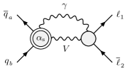
(d) Non-factorizable corrections

Figure 1: The four types of corrections that contribute to the mixed QCD–EW corrections in the PA illustrated in terms of generic two-loop amplitudes. Simple circles symbolize tree structures, double circles one-loop corrections, and triple circles two-loop contributions.

In detail, the four types of corrections are characterized as follows:

1. The initial–initial factorizable corrections are given by two-loop ${\mathcal{O}\!\left(\alpha_{\mathrm{s}}\alpha\right)}$ corrections to on-shell ${\mathrm{W}}/{\mathrm{Z}}$ production and the corresponding one-loop real–virtual and tree-level double-real contributions, i.e. ${\mathrm{W}}/{\mathrm{Z}}+{\mathrm{jet}}$ production at ${\mathcal{O}\!\left(\alpha\right)}$, ${\mathrm{W}}/{\mathrm{Z}}+\gamma$ production at ${\mathcal{O}\!\left(\alpha_{\mathrm{s}}\right)}$, and the processes ${\mathrm{W}}/{\mathrm{Z}}+\gamma+{\mathrm{jet}}$ at tree level. Results for individual ingredients of the initial–initial part are known, however, a consistent combination of these building blocks requires also a subtraction scheme for infrared (IR) singularities at ${\mathcal{O}\!\left(\alpha_{\mathrm{s}}\alpha\right)}$ and has not been performed yet. Note that currently no PDF set including ${\mathcal{O}\!\left(\alpha_{\mathrm{s}}\alpha\right)}$ corrections is available, which is required to absorb IR singularities of the initial–initial corrections from QCD and photon radiation collinear to the beams.

   Results of the PA at ${\mathcal{O}\!\left(\alpha\right)}$ show that observables such as the transverse-mass distribution in the case of W production or the lepton-invariant-mass distributions for Z production are extremely insensitive to photonic initial-state radiation (ISR) [8]. Since these distributions also receive relatively moderate QCD corrections, we do not expect significant initial–initial NNLO ${\mathcal{O}\!\left(\alpha_{\mathrm{s}}\alpha\right)}$ corrections to such distributions. For observables sensitive to initial-state recoil effects, such as the transverse-lepton-momentum distribution, the ${\mathcal{O}\!\left(\alpha_{\mathrm{s}}\alpha\right)}$ corrections should be larger, but still very small compared to the huge QCD corrections.

2. The factorizable initial–final corrections consist of the ${\mathcal{O}\!\left(\alpha_{\mathrm{s}}\right)}$ corrections to ${\mathrm{W}}/{\mathrm{Z}}$ production combined with the ${\mathcal{O}\!\left(\alpha\right)}$ corrections to the leptonic ${\mathrm{W}}/{\mathrm{Z}}$ decay. The latter comprise the by far dominant contribution to the PA at ${\mathcal{O}\!\left(\alpha\right)}$ with a substantial impact on the shape of differential distributions. Further given that the NLO QCD correction are sizable with no apparent suppression, we expect the factorizable corrections of “initial–final” type to capture the dominant ${\mathcal{O}\!\left(\alpha_{\mathrm{s}}\alpha\right)}$ effects. These NNLO corrections receive double-virtual, real–virtual, and double-real contributions, as illustrated in Fig. 2 in terms of generic interference diagrams. The cancellation of IR singularities between these individual contributions is achieved using a local subtraction scheme resulting in a fully differential calculation. In order to construct our NNLO subtraction terms we employ a two-fold application of the dipole subtraction formalism for NLO QCD and EW corrections. An important ingredient for this construction was the recent generalization of the formalism to cover decay kinematics, which has been worked out in Ref. [11]. Further details on the computation can be found in Ref. [2]. In the following sections we review the main results presented there.

   

   

   (a) Factorizable initial–final double-virtual corrections

   

   

   (b) Factorizable initial–final (real QCD)$\times$(virtual EW) corrections

   

   (c) Factorizable initial–final (virtual QCD)$\times$(real photonic) corrections

   

   

   (d) Factorizable initial–final double-real corrections

   Figure 2: Interference diagrams for the various contributions to the factorizable initial–final corrections of ${\mathcal{O}\!\left(\alpha_{\mathrm{s}}\alpha\right)}$, with blobs representing all relevant tree structures. The blobs with “$\alpha$” inside represent one-loop corrections of ${\mathcal{O}\!\left(\alpha\right)}$, and the double slash on a propagator line indicates that the corresponding momentum is set on its mass shell in the rest of the diagram (but not on the slashed line itself).

3. Factorizable final–final corrections arise solely from the ${\mathcal{O}\!\left(\alpha_{\mathrm{s}}\alpha\right)}$ counterterms of the lepton–${\mathrm{W}}/{\mathrm{Z}}$-boson vertices, which involve only corrections to the vector-boson self-energies at this order. Not only are these corrections free of IR divergences, but owing to the fact that there are no corresponding real contributions, the final–final corrections have practically no impact on the shape of distributions. The explicit calculation carried out in Ref. [2] further reveals that those corrections are in fact phenomenologically negligible.

4. The non-factorizable ${\mathcal{O}\!\left(\alpha_{\mathrm{s}}\alpha\right)}$ corrections are given by soft-photon corrections connecting the initial state, the intermediate vector boson, and the final-state leptons, combined with QCD corrections to $V$-boson production. As shown in detail in Ref. [8], these corrections can be expressed in terms of soft-photon correction factors to squared tree-level or one-loop QCD matrix elements by using gauge-invariance arguments. Furthermore, exploiting this factorization property, the IR cancellation can be accomplished by using a composition of two NLO methods: We employ the dipole-subtraction formalism for the treatment of the IR singularities associated with the QCD corrections together with the soft-slicing approach for the photonic corrections. The numerical impact of these corrections was found to be below the $0.1\%$ level and is therefore negligible for all phenomenological purposes.

3 Numerical results

3.1 Setup and conventions

The detailed setup and the input parameters used to obtain the results discussed in the following can be found in Ref. [2]. Here we just repeat the basic definition of the individual components of the QCD and EW corrections.

Our default prediction for the Drell–Yan cross section at mixed QCD–EW NNLO is obtained by adding the ${\mathcal{O}\!\left(\alpha_{\mathrm{s}}\alpha\right)}$ corrections $\Delta\sigma_{\text{prod}\times\text{dec}}^{\text{NNLO}_{\mathrm{s}\otimes\mathrm{ew}}}$ to the sum $\Delta\sigma^{\text{NLO}_{\mathrm{s}}}+\Delta\sigma^{\text{NLO}_{\mathrm{ew}}}$ of the full NLO QCD and EW corrections,

$$\sigma^{{\text{NNLO}}_{\mathrm{s}\otimes\mathrm{ew}}} =\sigma^{0}+\Delta\sigma^{\text{NLO}_{\mathrm{s}}}+\Delta\sigma^{\text{NLO}_{\mathrm{ew}}}+\Delta\sigma_{\text{prod}\times\text{dec}}^{\text{NNLO}_{\mathrm{s}\otimes\mathrm{ew}}},$$ (3)

where all terms are consistently evaluated with NLO PDFs including the leading-order (LO) contribution $\sigma^{0}$. The non-factorizable corrections as well as the factorizable corrections of “final–final” type are not taken into account due to their negligible size, as discussed above.

In order to validate estimates of the NNLO QCD–EW corrections based on a naive product ansatz, we define the naive product of the NLO QCD cross section and the relative EW corrections,

$$\sigma_{\text{naive fact}}^{\text{NNLO}_{\mathrm{s}\otimes\mathrm{ew}}} =\sigma^{\text{NLO}_{\mathrm{s}}}(1+\delta_{\alpha})=\sigma^{0}+\Delta\sigma^{\text{NLO}_{\mathrm{s}}}+\Delta\sigma^{\text{NLO}_{\mathrm{ew}}}+\Delta\sigma^{\text{NLO}_{\mathrm{s}}}\;\delta_{\alpha}.$$ (4)

The relative NLO EW corrections

$$\delta_{\alpha} \equiv\frac{\Delta\sigma^{\text{NLO}_{\mathrm{ew}}}}{\sigma^{0}}$$ (5)

are defined in two different versions: First, based on the full ${\mathcal{O}\!\left(\alpha\right)}$ correction ($\delta_{\alpha}$), and second, based on the dominant EW final-state correction of the PA ($\delta_{\alpha}^{\text{dec}}$).

Defining the correction factors,

$$\delta^{{\text{prod}}\times{\text{dec}}}_{\alpha_{\mathrm{s}}\alpha} \equiv\frac{\Delta\sigma_{{\text{prod}}\times{\text{dec}}}^{\text{NNLO}_{{\mathrm{s}}\otimes{\mathrm{ew}}}}}{\sigma^{\text{LO}}}, \delta_{\alpha_{\mathrm{s}}}^{\prime} \equiv\frac{\Delta\sigma^{\text{NLO}_{\mathrm{s}}}}{\sigma^{\text{LO}}},$$ (6)

we can cast the relative difference of our best prediction (3) and the product ansatz (4) into the following form,

$$\frac{\sigma^{\text{NNLO}_{\mathrm{s}\otimes\mathrm{ew}}}-\sigma_{\text{naive fact}}^{\text{NNLO}_{\mathrm{s}\otimes\mathrm{ew}}}}{\sigma^{\text{LO}}} =\delta^{{\text{prod}}\times{\text{dec}}}_{\alpha_{\mathrm{s}}\alpha}-\delta_{\alpha_{\mathrm{s}}}^{\prime}\delta_{\alpha},$$ (7)

where the LO prediction $\sigma^{\text{LO}}$ in the denominators is evaluated with the LO PDFs. The difference of the relative NNLO correction $\delta^{\text{prod}\times\text{dec}}_{\alpha_{\mathrm{s}}\alpha}$ and the naive product $\delta_{\alpha_{\mathrm{s}}}^{\prime}\delta_{\alpha}^{(\text{dec})}$ therefore allows to assess the validity of a naive product ansatz.

Most contributions to the factorizable initial–final corrections take the reducible form of a product of two NLO corrections, with the exception of the double-real emission corrections which are defined with the full kinematics of the $2\to 4$ phase space. It is only in the double-real contributions where the final-state leptons receive recoils from both QCD and photonic radiation, an effect that cannot be captured by naively multiplying NLO QCD and EW corrections. Any large deviations between $\delta^{\text{prod}\times\text{dec}}_{\alpha_{\mathrm{s}}\alpha}$ and $\delta_{\alpha_{\mathrm{s}}}^{\prime}\delta_{\alpha}^{(\text{dec})}$ can therefore be attributed to this type of contribution. The difference of the naive products defined in terms of $\delta_{\alpha}^{\text{dec}}$ and $\delta_{\alpha}$ allows us to assess the impact of the missing ${\mathcal{O}\!\left(\alpha_{\mathrm{s}}\alpha\right)}$ corrections beyond the initial–final corrections considered in our calculation and therefore also provides an error estimate of the PA, and in particular of the omission of the corrections of “initial–initial” type.

3.2 Results on the dominating ${\mathcal{O}\!\left(\alpha_{\mathrm{s}}\alpha\right)}$ corrections

Figure 4 shows the numerical results for the relative ${\mathcal{O}\!\left(\alpha_{\mathrm{s}}\alpha\right)}$ initial–final factorizable corrections $\delta^{\text{prod}\times\text{dec}}_{\alpha_{\mathrm{s}}\alpha}$ to the transverse-mass ($M_{{\mathrm{T}},\nu\ell}$) and the transverse-lepton-momentum ($p_{{\mathrm{T}},\ell}$) distributions for $\mathrm{W^{+}}$ production at the LHC. The results for the neutral-current process are given in Fig. 4, which displays the results for the lepton-invariant-mass ($M_{\ell\ell}$) distribution and a transverse-lepton-momentum ($p_{{\mathrm{T}},\ell^{+}}$) distribution.

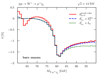
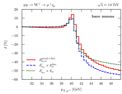
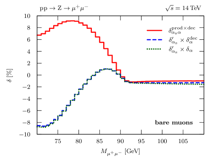
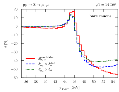
Figure 3: Relative factorizable corrections of ${\mathcal{O}\!\left(\alpha_{\mathrm{s}}\alpha\right)}$ induced by initial-state QCD and final-state EW contributions to the transverse-mass (left) and transverse-lepton-momentum (right) distributions for $\mathrm{W^{+}}$ production at the LHC. The naive products of the NLO correction factors $\delta_{\alpha_{\mathrm{s}}}^{\prime}$ and $\delta_{\alpha}$ are shown for comparison. (Taken from Ref. [2].)

Figure 4: Relative factorizable corrections of ${\mathcal{O}\!\left(\alpha_{\mathrm{s}}\alpha\right)}$ induced by initial-state QCD and final-state EW contributions to the lepton-invariant-mass distribution (left) and a transverse-lepton-momentum distribution (right) for $\mathrm{Z}$ production at the LHC. The naive products of the NLO correction factors $\delta_{\alpha_{\mathrm{s}}}^{\prime}$ and $\delta_{\alpha}$ are shown for comparison. (Taken from Ref. [2].)

In Figs. 4 and 4 we compare to the two different implementations of a naive product of correction factors discussed after Eq. (7). In both figures, we assume that final-state leptons and collinear photons can be resolved completely (defining “bare leptons”), a situation that is realistic for muons, but not for electrons, which appear in showers together with the photons in the electromagnetic calorimeter in the detector. For the latter case, results based on some recombination of leptons with collinear photons are more realistic (defining “dressed leptons”). Such results can be found in Ref. [2]. They show the same features as the ones for bare leptons, with corrections that are typically smaller by a factor of two.

For the $M_{{\mathrm{T}},\nu\ell}$ distribution for ${\mathrm{W^{+}}}$ production (left plot in Fig. 4), the mixed NNLO QCD–EW corrections are moderate and amount to approximately ${-1.7}~{}{\%}$ around the resonance, which is about an order of magnitude smaller than the NLO EW corrections. Both variants of the naive product provide a good approximation to the full result in the region around and below the Jacobian peak, which is dominated by resonant ${\mathrm{W}}$ production. For larger $M_{{\mathrm{T}},\nu\ell}$, the product $\delta_{\alpha_{\mathrm{s}}}^{\prime}\delta_{\alpha}$ based on the full NLO EW correction factor deviates from the other curves. Due to the well-known insensitivity of the observable $M_{{\mathrm{T}},\nu\ell}$ to ISR effects seen for the NLO corrections [8], this difference signals the growing importance of effects beyond the PA. However, the deviations amount to only few per-mille for $M_{{\mathrm{T}},\nu\ell}\lesssim{90}~{}{\,\mathrm{GeV}}$. The overall good agreement between the $\delta^{\text{prod}\times\text{dec}}_{\alpha_{\mathrm{s}}\alpha}$ corrections and both naive products can be attributed to well-known insensitivity of the observable $M_{{\mathrm{T}},\nu\ell}$ to ISR effects already seen in the case of NLO corrections in Ref. [8].

For the $p_{{\mathrm{T}},\ell}$ distributions (right plots in Figs. 4 and 4 for ${\mathrm{W^{+}}}$/${\mathrm{Z}}$ production, respectively) we observe corrections that are small far below the Jacobian peak, but which rise to about $15\%$ ($20\%$) on the Jacobian peak at $p_{{\mathrm{T}},\ell}\approx M_{V}/2$ for the case of the $\mathrm{W^{+}}$ boson ($\mathrm{Z}$ boson) and then display a steep drop reaching almost $-50\%$ at $p_{{\mathrm{T}},\ell}={50}~{}{\,\mathrm{GeV}}$. This enhancement stems from the large QCD corrections above the Jacobian peak familiar from the NLO QCD results (see e.g. Fig. 8 in Ref. [8]) where the recoil due to real QCD radiation shifts events with resonant ${\mathrm{W}}$/${\mathrm{Z}}$ bosons above the Jacobian peak. The naive product ansatz fails to provide a good description of the full result $\delta^{\text{prod}\times\text{dec}}_{\alpha_{\mathrm{s}}\alpha}$ and deviates by 5–10% at the Jacobian peak, where the PA is expected to be the most accurate. This can be attributed to the strong influence of the recoil induced by ISR on the transverse momentum, which implies a larger effect of the double-real emission corrections on this distribution that are not captured correctly by the naive products. The two versions of the naive products display larger deviations than in the $M_{{\mathrm{T}},\nu\ell}$ distribution discussed above, which signals a larger impact of the missing ${\mathcal{O}\!\left(\alpha_{\mathrm{s}}\alpha\right)}$ initial–initial corrections. However, these deviations should be interpreted with care, since a fixed-order prediction is not sufficient to describe this distribution around the peak region $p_{{\mathrm{T}},\ell}\approx M_{V}/2$, which corresponds to the kinematic onset for $V+\text{jet}$ production and is known to require QCD resummation for a proper description.

In case of the $M_{\ell\ell}$ distribution for ${\mathrm{Z}}$ production (left plot in Fig. 4), corrections up to $10\%$ are observed below the resonance for the case of bare muons. This is consistent with the large EW corrections at NLO in this region, which arise from photonic final-state radiation (FSR) that shifts the reconstructed value of the invariant lepton-pair mass away from the resonance to lower values. The naive product approximates the full initial–final corrections $\delta^{\text{prod}\times\text{dec}}_{\alpha_{\mathrm{s}}\alpha}$ reasonably well at the resonance itself ($M_{\ell\ell}=M_{\mathrm{Z}}$) and above, but completely fails already a little below the resonance where the naive products do not even reproduce the sign of the full $\delta^{\text{prod}\times\text{dec}}_{\alpha_{\mathrm{s}}\alpha}$ correction. This deviation occurs although the invariant-mass distribution is widely unaffected by ISR effects. The fact that we obtain almost identical corrections from the two versions of the product $\delta_{\alpha_{\mathrm{s}}}^{\prime}\delta_{\alpha}^{\text{dec}}$ and $\delta_{\alpha_{\mathrm{s}}}^{\prime}\delta_{\alpha}$ demonstrates the insensitivity of this observable to photonic ISR. The origin of the failure of the naive product ansatz, which is discussed in Ref. [2] in detail, can be understood as follows. The large EW corrections below the resonance arise due to the redistribution of events near the ${\mathrm{Z}}$ pole to lower lepton invariant masses by photonic FSR, so that it would be more appropriate to replace the QCD correction factor $\delta_{\alpha_{\mathrm{s}}}^{\prime}$ in the naive product by its value at the resonance $\delta_{\alpha_{\mathrm{s}}}^{\prime}(M_{\ell\ell}=M_{\mathrm{Z}})\approx 6.5\%$, which corresponds to the location of the events that are responsible for the bulk of the large EW corrections below the resonance. In contrast, the naive product ansatz simply multiplies the corrections locally on a bin-by-bin basis. The observed mismatch is dramatically enhanced by the fact that the QCD correction $\delta_{\alpha_{\mathrm{s}}}^{\prime}$ exhibits a sign change at $M_{\ell\ell}\approx{83}~{}{\,\mathrm{GeV}}$.

Contrary to the lepton-invariant-mass distribution, the transverse-mass distribution is dominated by events with resonant W bosons even in the range below the Jacobian peak, $M_{{\mathrm{T}},\nu\ell}\lesssim M_{\mathrm{W}}$, so that it is less sensitive to the redistribution of events to lower $M_{{\mathrm{T}},\nu\ell}$. This explains why the naive product can provide a good approximation of the full initial–final NNLO corrections. It should be emphasized, however, that even in the case of the $M_{{\mathrm{T}},\nu\ell}$ distribution any event selection criteria that deplete events with resonant W bosons below the Jacobian peak will result in increased sensitivity to the effects of FSR and can potentially lead to a failure of a naive product ansatz.

In conclusion, simple approximations in terms of products of correction factors have to be used with care and require a careful case-by-case investigation of their validity.

3.3 Approximating ${\mathcal{O}\!\left(\alpha_{\mathrm{s}}\alpha\right)}$ corrections by leading logarithmic final-state radiation

As is evident from Figs. 4 and 4, a naive product of QCD and EW correction factors (4) is not adequate to approximate the NNLO QCD–EW corrections for all observables. A promising approach to a factorized approximation for the dominant initial–final corrections can be obtained by combining the full NLO QCD corrections to vector-boson production with the leading-logarithmic (LL) approximation for FSR. The benefit in this approximation lies in the fact that the interplay of the recoil effects from jet and photon emission is properly taken into account. On the other hand, the LL approximation neglects certain (non-universal) finite contributions, which are, however, suppressed with respect to the dominating radiation effects.

In the following we compare two standard approaches to include FSR off leptons in LL approximation: the structure-function and the parton-shower approaches. In the former, generated events are dressed with FSR effects by convoluting the differential cross section by a structure function describing the energy loss of the leptons by collinear photon emission. Since the structure-function approach works with strictly collinear photon emission, by construction the impact of LL FSR is zero for dressed leptons, where the mass-singluar logarithm of the lepton cancels by virtue of the KLN theorem because of the inclusive treatment of the collinear lepton–photon system. In contrast, photons generated through parton-shower approaches to photon radiation (see e.g. Refs. [12, 13, 14]) also receive momentum components transverse to the original lepton momentum, following the differential factorization formula, so that the method is also applicable to the case of collinear-safe observables, i.e. to the dressed-lepton case. For this purpose, we have implemented the combination of the exact NLO QCD prediction for vector-boson production with the simulation of FSR using PHOTOS [15]. Since we are interested in comparing to the ${\mathcal{O}\!\left(\alpha_{\mathrm{s}}\alpha\right)}$ corrections in our setup, we only generate a single photon emission using PHOTOS and use the same input-parameter scheme for $\alpha$ (see Ref. [2] for details).

In Figs. 6 and 6 we compare our best prediction (3) for the factorizable initial–final ${\mathcal{O}\!\left(\alpha_{\mathrm{s}}\alpha\right)}$ corrections to the combination of NLO QCD corrections with the approximate FSR obtained from the structure-function approach and PHOTOS for the case of ${\mathrm{W^{+}}}$ production and ${\mathrm{Z}}$ production, respectively.

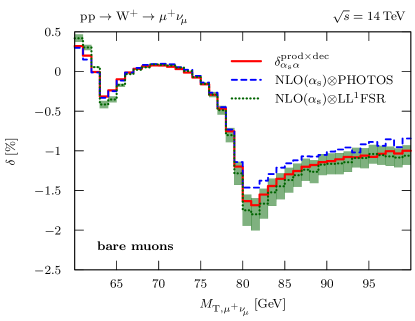
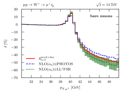
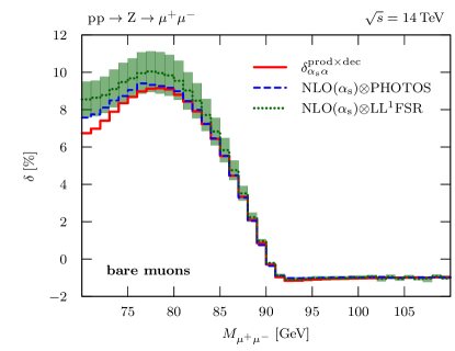
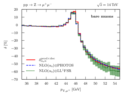
Figure 5: Comparison of the approximation obtained from PHOTOS and from the structure-function approach ($\mathrm{LL}^{1}\mathrm{FSR}$) for the relative ${\mathcal{O}\!\left(\alpha_{\mathrm{s}}\alpha\right)}$ initial-state QCD and final-state EW corrections to our best prediction $\delta^{\mathrm{prod\times dec}}_{\alpha_{\mathrm{s}}\alpha}$ for the case of the transverse-mass (left) and transverse-lepton-momentum (right) distributions for $\mathrm{W^{+}}$ production at the LHC. (Taken from Ref. [2].)

Figure 6: Comparison of the approximation obtained from PHOTOS and from the structure-function approach ($\mathrm{LL}^{1}\mathrm{FSR}$) for the relative ${\mathcal{O}\!\left(\alpha_{\mathrm{s}}\alpha\right)}$ initial-state QCD and final-state EW corrections to our best prediction $\delta^{\mathrm{prod\times dec}}_{\alpha_{\mathrm{s}}\alpha}$ for the case of the lepton-invariant-mass distribution (left) and a transverse-lepton-momentum distribution (right) for $\mathrm{Z}$ production at the LHC. (Taken from Ref. [2].)

The corresponding results for dressed leptons can be found in Ref. [2]. The combination of the NLO QCD corrections and approximate FSR leads to a clear improvement compared to the naive product approximations investigated in the previous section. This is particularly apparent in the neutral-current process where the $M_{\ell\ell}$ distribution is correctly modelled by both LL FSR approximations, whereas the naive products shown in Figs. 4 completely failed to describe this distribution. In the $M_{{\mathrm{T}},\nu\ell}$ spectrum of the charged-current process in Fig. 6 one also finds good agreement of the different results below the Jacobian peak and an improvement over the naive product approximations in Fig. 4. The description of the $p_{{\mathrm{T}},\ell}$ distributions is also improved compared to the naive product approximations, but some differences remain in the charged-current process.

In spite of the good agreement of the two versions of incorporating FSR effects, the intrinsic uncertainty of the LL approximations should be kept in mind. For the structure-function approach, this uncertainty is illustrated by the band width resulting from the uncertainty in the QED scale $Q$, which is not determined at the LL level and varied within the range $M_{V}/2<Q<2M_{V}$ for $V={\mathrm{W}},{\mathrm{Z}}$. We remark that the multi-photon corrections obtained by employing the structure function with effects beyond ${\mathcal{O}\!\left(\alpha\right)}$ lie well within the aforementioned scale bands, which shows that a proper matching to the full NLO EW calculation is needed to remove the dominant uncertainty of the LL approximation and to predict the higher-order effects reliably. For PHOTOS the intrinsic uncertainty is not shown and not easy to quantify. The good quality of the PHOTOS approximation results from the fact that the finite terms in the photon emission probability are specifically adapted to ${\mathrm{W}}/{\mathrm{Z}}$-boson decays. The level of agreement with our “full prediction”, thus, cannot be taken over to other processes.

3.4 Impact on the W-boson mass extraction

In order to estimate the effect of the ${\mathcal{O}\!\left(\alpha_{\mathrm{s}}\alpha\right)}$ corrections on the extraction of the ${\mathrm{W}}$-boson mass at the LHC we have performed a $\chi^{2}$ fit of the $M_{{\mathrm{T}},\nu\ell}$ distribution. We treat the $M_{{\mathrm{T}},\nu\ell}$ spectra calculated in various theoretical approximations for a reference mass $M_{\mathrm{W}}^{\text{OS}}=80.385~\,\mathrm{GeV}$ as “pseudo-data” that we fit with “templates” calculated using the LO predictions $\sigma^{0}$ (with NLO PDFs) for different values of $M_{\mathrm{W}}^{\text{OS}}$. Specifically, we have generated results for $27$ transverse-mass bins in the interval $M_{{\mathrm{T}},\nu\ell}=[64,\,91]~\,\mathrm{GeV}$ in steps of $1~\,\mathrm{GeV}$, varying the ${\mathrm{W}}$-boson mass in the interval $M_{\mathrm{W}}=[80.085,\,80.785]~\,\mathrm{GeV}$ with steps of $\Delta M_{\mathrm{W}}=10~\,\mathrm{MeV}$ (steps of $\Delta M_{\mathrm{W}}=5~\,\mathrm{MeV}$ in the interval $M_{\mathrm{W}}=[80.285,\,80.485]~\,\mathrm{GeV}$). Using a linear interpolation between neighbouring $M_{\mathrm{W}}$ values, we obtain the integrated cross sections in the $i$-th $M_{{\mathrm{T}},\nu\ell}$ bin, $\sigma_{i}^{0}(M_{\mathrm{W}})$, as a continuous function of $M_{\mathrm{W}}$. The best-fit value $M_{\mathrm{W}}^{\mathrm{fit},\mathrm{th}}$ quantifying the impact of a higher-order correction in the theoretical cross section $\sigma^{\mathrm{th}}$ is then obtained from the minimum of the function

$$\chi^{2}(M_{\mathrm{W}}^{\mathrm{fit},\mathrm{th}})=\sum_{i}\frac{\left[\sigma_{i}^{\mathrm{th}}(M_{\mathrm{W}}^{\text{OS}})-\sigma_{i}^{0}(M_{\mathrm{W}}^{\mathrm{fit},\mathrm{th}})\right]^{2}}{2\Delta\sigma_{i}^{2}}\,,$$ (8)

where the sum over $i$ runs over the transverse-mass bins. Here $\sigma_{i}^{\mathrm{th}}$ and $\sigma_{i}^{0}$ are the integrated cross sections in the $i$-th bin, uniformly rescaled so that the sum over all $27$ bins is identical for all considered cross sections. We assume a statistical error of the pseudo-data and take $\Delta\sigma_{i}^{2}\propto\sigma_{i}^{\mathrm{th}}$. We have also performed a two-parameter fit where the normalization of the templates is fitted simultaneously, leading to identical results. Similarly, allowing the ${\mathrm{W}}$-boson width in the templates to float and fitting $M_{\mathrm{W}}$ and $\Gamma_{{\mathrm{W}}}$ simultaneously does not significantly affect our results on the mass shift.

In the experimental measurements of the transverse-mass distribution, the Jacobian peak is washed out due to the finite energy and momentum resolution of the detectors. In our simple estimate of the impact of higher-order corrections on the extracted value of the ${\mathrm{W}}$-boson mass, we do not attempt to model such effects. We expect the detector effects to affect the different theory predictions in a similar way and to cancel to a large extent in our estimated mass shift, which is obtained from a difference of mass values extracted from pseudo-data calculated using different theory predictions. This assumption is supported by the fact that our estimate of the effect of the NLO EW corrections is similar to the one obtained in Ref. [13] using a Gaussian smearing of the four-momenta to simulate detector effects.

	bare muons		dressed leptons
	$M^{\mathrm{fit}}_{\mathrm{W}}\;[\mathrm{GeV}]$	$\qquad\Delta M_{\mathrm{W}}$	$M^{\mathrm{fit}}_{\mathrm{W}}\;[\mathrm{GeV}]$	$\qquad\Delta M_{\mathrm{W}}$
LO	$80.385$	$\bigg{\}}\;-90~{}\mathrm{MeV}$	$80.385$	$\bigg{\}}\;-40~{}\mathrm{MeV}$
$\text{NLO}_{\mathrm{ew}}$	$80.295$		$80.345$
$\text{NLO}_{\mathrm{s}\oplus\mathrm{ew}}$	$80.374$	$\biggr{\}}\;-14~{}\mathrm{MeV}$	$80.417$	$\biggr{\}}\;-4~{}\mathrm{MeV}$
NNLO	$80.360$		$80.413$

Table 1: Values of the ${\mathrm{W}}$-boson mass in GeV obtained from the $\chi^{2}$ fit of the $M_{{\mathrm{T}},\nu\ell}$ distribution in different theoretical approximations to LO templates and the resulting mass shifts. (Taken from Ref. [2].)

The fit results for several NLO approximations and our best NNLO prediction (3) are given in Table 1. To validate our procedure we estimate the mass shift due to the NLO EW corrections by using the prediction $\sigma^{\text{NLO}_{\mathrm{ew}}}=\sigma^{0}+\Delta\sigma^{\text{NLO}_{\mathrm{ew}}}$ as the pseudo-data $\sigma^{\mathrm{th}}$ in (8). The corresponding $\chi^{2}$ distributions as a function of the mass shift $\Delta M_{\mathrm{W}}^{\text{NLO}_{\mathrm{ew}}}$ can be found in Ref. [2]. From the minima of the distributions one finds a mass shift of $\Delta M_{\mathrm{W}}^{\text{NLO}_{\mathrm{ew}}}\approx-90~\,\mathrm{MeV}$ for bare muons and $\Delta M_{\mathrm{W}}^{\text{NLO}_{\mathrm{ew}}}\approx-40~\,\mathrm{MeV}$ for dressed muons. These values are comparable to previous results reported in Ref. [13]. Alternatively, the effect of the EW corrections can be estimated by comparing the value of $M_{\mathrm{W}}$ obtained from a fit to the naive product of EW and QCD corrections (4) to the result of a fit to the NLO QCD cross section. The results are consistent with the shift estimated from the NLO EW corrections alone.

We have also estimated the effect of multi-photon radiation on the $M_{\mathrm{W}}$ measurement in the bare-muon case using the structure-function approach. We obtain a mass shift $\Delta M_{\mathrm{W}}^{\mathrm{FSR}}\approx 9~\,\mathrm{MeV}$ relative to the result of the fit to the NLO EW prediction, which is in qualitative agreement with the result of Ref. [13].

To estimate the impact of the initial–final ${\mathcal{O}\!\left(\alpha_{\mathrm{s}}\alpha\right)}$ corrections we consider the mass shift relative to the full NLO result,

$$\Delta M_{\mathrm{W}}^{\text{NNLO}}=M_{\mathrm{W}}^{\mathrm{fit},\text{NNLO}_{\mathrm{s}\otimes\mathrm{ew}}^{\text{prod}\times\text{dec}}}-M_{\mathrm{W}}^{\mathrm{fit},\text{NLO}_{\mathrm{s}\oplus\mathrm{ew}}},$$ (9)

where $M_{\mathrm{W}}^{\mathrm{fit},\text{NNLO}_{\mathrm{s}\otimes\mathrm{ew}}^{\text{prod}\times\text{dec}}}$ is the result of using our best prediction (3) to generate the pseudo-data, while the sum of the NLO QCD and EW corrections is used for $\Delta M_{\mathrm{W}}^{\mathrm{fit},\text{NLO}_{\mathrm{s}\oplus\mathrm{ew}}}$. The resulting $\chi^{2}$ distributions for the mass shift can again be found in Ref. [2]. In the bare-muon case, we obtain a mass shift due to ${\mathcal{O}\!\left(\alpha_{\mathrm{s}}\alpha\right)}$ corrections of $\Delta M_{\mathrm{W}}^{\mathrm{NNLO}}\approx-14~\,\mathrm{MeV}$, while for the dressed-lepton case we get $\Delta M_{\mathrm{W}}^{\mathrm{NNLO}}\approx-4~\,\mathrm{MeV}$.

Identical shifts result from replacing the NNLO prediction by the naive product (4), which is expected from the good agreement for the $M_{{\mathrm{T}},\nu\ell}$-spectrum in Fig. 4. Using instead the LL approximation of the FSR obtained using PHOTOS to compute the ${\mathcal{O}\!\left(\alpha_{\mathrm{s}}\alpha\right)}$ corrections, we obtain a mass shift of $\Delta M_{\mathrm{W}}^{\text{NNLO}}=-11~\,\mathrm{MeV}$ ($-4~\,\mathrm{MeV}$) for the bare-muon (dressed-lepton) case. The effect of the ${\mathcal{O}\!\left(\alpha_{\mathrm{s}}\alpha\right)}$ corrections on the mass measurement is therefore of a similar or larger magnitude than the effect of multi-photon radiation. We emphasize that the result $\Delta M_{\mathrm{W}}^{\text{NNLO}}\approx-14~\,\mathrm{MeV}$ is a simple estimate of the impact of the full ${\mathcal{O}\!\left(\alpha_{\mathrm{s}}\alpha\right)}$ corrections on the $M_{\mathrm{W}}$ measurement. The order of magnitude shows that these corrections must be taken into account properly in order to reach the $10~\,\mathrm{MeV}$ accuracy goal of the LHC experiments.

4 Conclusions

The Drell–Yan-like ${\mathrm{W}}$- and ${\mathrm{Z}}$-boson production processes are among the most precise probes of the Standard Model and do not only serve as key benchmark or “standard candle” processes, but further allow for precision measurements of the ${\mathrm{W}}$-boson mass and the effective weak mixing angle. In view of the envisioned accuracy of these measurements, a further improvement of the theory prediction is mandatory. To this end, the mixed QCD–electroweak corrections of ${\mathcal{O}\!\left(\alpha_{\mathrm{s}}\alpha\right)}$ represent the largest component of fixed-order radiative corrections after the well established NNLO QCD and NLO electroweak corrections.

In this article, we have reviewed the major results of our two recent papers [8, 2], where we have established a framework for evaluating the ${\mathcal{O}\!\left(\alpha_{\mathrm{s}}\alpha\right)}$ corrections to Drell–Yan processes in the resonance region using a pole approximation and presented the calculation of the non-factorizable and most important factorizable corrections. The non-factorizable corrections and the factorizable corrections solely associated with the W/Z decay subprocesses, which were computed in Ref. [8] and [2], respectively, turned out to be phenomenologically negligible. Moreover, an analysis of the NLO corrections in pole approximation suggests that the factorizable corrections corresponding to the production subprocess, which are yet unknown, will have a minor impact on the observables relevant for the W-boson mass measurement. The dominant factorizable corrections of ${\mathcal{O}\!\left(\alpha_{\mathrm{s}}\alpha\right)}$ are the ones resulting from the combination of sizable QCD corrections to the production with large EW corrections to the decay subprocesses, explicitly calculated in Ref. [2]. Here we have summarized the numerical results for so-called bare leptons and the most important observables for the ${\mathrm{W}}$-boson mass measurement: the transverse-mass and lepton-transverse-momentum distributions for $\mathrm{W}$ production. The results for the neutral-current process comprise the invariant-mass and the lepton-transverse-momentum distributions.

We have shown that naive products fail to capture the factorizable initial–final corrections in distributions such as in the transverse momentum of the lepton, which are sensitive to QCD initial-state radiation and therefore require a correct treatment of the double-real-emission part of the NNLO corrections. Naive products also fail to capture observables that are strongly affected by a redistribution of events due to final-state real-emission corrections, such as the invariant-mass distribution of the neutral-current process. On the other hand, if an observable is less affected by such a redistribution of events or is only affected by it in the vicinity of the resonance, such as the transverse-mass distribution of the charged-current process, the naive products are able to reproduce the factorizable initial–final corrections to a large extent. Moreover, we have investigated to which extent the factorizable initial–final corrections calculated in this paper can be approximated by a combination of the NLO QCD corrections and a collinear approximation of real-photon emission through a QED structure-function approach or a QED parton shower such as PHOTOS. For the invariant-mass distribution in ${\mathrm{Z}}$-boson production we observe a significant improvement in the agreement compared to the naive product ansatz, since both PHOTOS and the QED structure function model the redistribution of events due to final-state radiation, which is responsible for the bulk of the corrections in this observable. Our results can furthermore be used to validate Monte Carlo event generators where ${\mathcal{O}\!\left(\alpha_{\mathrm{s}}\alpha\right)}$ corrections are approximated by a combination of NLO matrix elements and parton showers.

Finally, we have illustrated the phenomenological impact of the ${\mathcal{O}\!\left(\alpha_{\mathrm{s}}\alpha\right)}$ corrections by estimating the mass shift induced by the factorizable initial–final corrections as $\approx-14~\,\mathrm{MeV}$ for the case of bare muons and $\approx-4~\,\mathrm{MeV}$ for dressed leptons. These corrections therefore have to be properly taken into account in the ${\mathrm{W}}$-boson mass measurements at the LHC, which aim at a precision of about $10~\,\mathrm{MeV}$. It will be interesting to investigate the impact of the ${\mathcal{O}\!\left(\alpha_{\mathrm{s}}\alpha\right)}$ corrections on the measurement of the effective weak mixing angle as well in the future.

References

- [1] M. Baak et al., arXiv:1310.6708 [hep-ph].
- [2] S. Dittmaier, A. Huss and C. Schwinn, arXiv:1511.08016 [hep-ph], to appear in Nucl. Phys. B.
- [3] A. Kotikov, J. H. Kühn and O. Veretin, Nucl. Phys. B 788 (2008) 47 doi:10.1016/j.nuclphysb.2007.07.018 [hep-ph/0703013 [HEP-PH]].
- [4] W. B. Kilgore and C. Sturm, Phys. Rev. D 85 (2012) 033005 doi:10.1103/PhysRevD.85.033005 [arXiv:1107.4798 [hep-ph]].
- [5] R. Bonciani, PoS EPS -HEP2011 (2011) 365.
- [6] A. Czarnecki and J. H. Kühn, Phys. Rev. Lett. 77 (1996) 3955 doi:10.1103/PhysRevLett.77.3955 [hep-ph/9608366].
- [7] D. Kara, Nucl. Phys. B 877 (2013) 683 doi:10.1016/j.nuclphysb.2013.10.024 [arXiv:1307.7190 [hep-ph]].
- [8] S. Dittmaier, A. Huss and C. Schwinn, Nucl. Phys. B 885 (2014) 318 doi:10.1016/j.nuclphysb.2014.05.027 [arXiv:1403.3216 [hep-ph]].
- [9] U. Baur, S. Keller and D. Wackeroth, Phys. Rev. D 59 (1999) 013002 doi:10.1103/PhysRevD.59.013002 [hep-ph/9807417].
- [10] S. Dittmaier and M. Krämer, Phys. Rev. D 65 (2002) 073007 doi:10.1103/PhysRevD.65.073007 [hep-ph/0109062].
- [11] L. Basso, S. Dittmaier, A. Huss and L. Oggero, arXiv:1507.04676 [hep-ph], to appear in Eur. Phys. J. C.
- [12] W. Placzek and S. Jadach, Eur. Phys. J. C 29 (2003) 325 doi:10.1140/epjc/s2003-01223-4 [hep-ph/0302065].
- [13] C. M. Carloni Calame, G. Montagna, O. Nicrosini and M. Treccani, Phys. Rev. D 69 (2004) 037301 doi:10.1103/PhysRevD.69.037301 [hep-ph/0303102].
- [14] C. M. Carloni Calame, G. Montagna, O. Nicrosini and M. Treccani, JHEP 0505 (2005) 019 doi:10.1088/1126-6708/2005/05/019 [hep-ph/0502218].
- [15] P. Golonka and Z. Was, Eur. Phys. J. C 45 (2006) 97 doi:10.1140/epjc/s2005-02396-4 [hep-ph/0506026].