Accuracy of the Post-Newtonian Approximation for Extreme-Mass Ratio Inspirals from Black-hole Perturbation Approach

Abstract

We revisit the accuracy of the post-Newtonian (PN) approximation and its region of validity for quasi-circular orbits of a point particle in the Kerr spacetime, by using an analytically known highest post-Newtonian order gravitational energy flux and accurate numerical results in the black hole perturbation approach. It is found that regions of validity become larger for higher PN order results although there are several local maximums in regions of validity for relatively low-PN order results. This might imply that higher PN order calculations are also encouraged for comparable-mass binaries.

I Introduction

To understand binary systems in General Relativity analytically, we require perturbative techniques. The post-Newtonian (PN) approximation based on a perturbative expansion by assuming slow motions and weak gravitational fields of physical systems, is one of the most successful approaches (see e.g., Refs. Blanchet:2013haa ; Sasaki:2003xr for a review). In this approximation, formally $1/c$ where $c$ is the speed of light, is considered as a small parameter that goes to zero in the Newtonian limit $c\to\infty$. This PN approach has been used to construct accurate inspiral waveforms of binaries which are one of the important gravitational wave sources for the second generation gravitational wave detectors such as Advanced LIGO (aLIGO) TheLIGOScientific:2014jea , Advanced Virgo (AdV) TheVirgo:2014hva , KAGRA Somiya:2011np ; Aso:2013eba .

The orbital separation of binary systems decreases gradually by the radiation reaction due to the emission of gravitational waves. As the orbital separation decreases, the PN approximation will be inappropriate because the slow-motion/weak-field assumptions are violated. Therefore, we have a basic question: “How far can we push the PN approximation in the fast-motion/strong-field?”

In this paper, we treat extreme mass ratio inspirals (EMRIs) as binary systems to discuss the region of validity of the PN approximation. For the above systems which are one of the main targets for a space-based mission, eLISA Ref. Seoane:2013qna , the black hole perturbation approach is applicable. In this approach, we consider a point particle with mass $\mu$ is orbiting around a black hole with mass $M$, where $\mu\ll M$. As an example, in the leading order with respect to the $\mu/M$ expansion, we consider a quasi-circular orbit of the particle in the Kerr spacetime with Kerr parameter $a$. Due to the gravitational radiation reaction, the particle will reach the innermost stable circular orbit (ISCO) finally. In the case of equatorial orbits in Kerr spacetime, the orbital radius is obtained as Bardeen:1972fi

$$\frac{r_{\rm ISCO}}{M}= 3+Z_{2}\mp\sqrt{(3-Z_{1})(3+Z_{1}+2Z_{2})}\,;$$ (1)

$$Z_{1}= 1+(1-(a/M)^{2})^{1/3}$$ (2)

$$\times[(1+a/M)^{1/3}+(1-a/M)^{1/3}]\,,$$ (3)

$$Z_{2}= \sqrt{3(a/M)^{2}+Z_{1}^{2}}\,,$$ (4)

(we use $c=G=1$ in this paper). Here, the upper and lower signs refer to the direct and retrograde orbits (with $0\leq a\leq M$), respectively. We have $r_{\rm ISCO}/M=1$ (direct) and $9$ (retrograde) for $a/M=1$. The gravitational field along this orbit is so strong that the PN approximation has the potential to be inappropriate. The evolution after the ISCO will be described by the “inspiral to plunge” transition model developed by Buonanno:2000ef ; Ori:2000zn ; Kesden:2011ma .

There are some works on the region of validity of the PN approximation in the case of EMRIs. Poisson Poisson:1995vs demonstrated that the convergence of the PN formula of the energy flux seems to be poor for $v>0.2$. In the asymptotic analysis of the PN energy flux, Yunes and Berti Yunes:2008tw found that the edges of the region of validity decrease with PN orders beyond 3PN by using the 5.5PN order result, and the optimal asymptotic approximation is the 3PN order result. It is possible to consider the PN series as a divergent asymptotic series (for example, see Ref. BenderOrszag and Section 2 of Ref. Yunes:2008tw ). This work has been extended to the case of quasi-circular orbits in the Kerr spacetime by Zhang, Yunes and Berti Zhang:2011vha .

Here, one of the authors of this paper derived the 14PN order energy flux for a test particle in a circular orbit around a Schwarzschild black hole Fujita:2011zk . Until this work, the highest PN order computation was up to the 5.5PN order Tanaka:1997dj . According to the 14PN result in Fig. 1 of Ref. Fujita:2011zk , we can see a better convergent behavior in the higher PN order than Fig. 1 of Ref. Mino:1997bx . Ref. Fujita:2011zk has been extended to even higher PN order, i.e., 22PN order for circular orbits around a Schwarzschild black hole Fujita:2012cm and 11PN for circular orbits around a Kerr black hole Fujita:2014eta . Recently, the 4PN calculation for general inclined orbits with the sixth order of the eccentricity has been done in Ref. Sago:2015rpa . Therefore, it is worth while to revisit the region of validity of the PN approximation with this higher PN order result.

The paper is organized as follows. In Sec. II, we review Refs. Yunes:2008tw ; Zhang:2011vha and summarize some definitions used in our paper. The state-of-the-art PN calculation for the Kerr case in Ref. Fujita:2014eta and the computation of the numerical energy flux in Refs. Fujita:2004rb ; Fujita:2009uz for circular orbit in the Kerr spacetime are used to obtain an improved estimation. Although we use the region of validity defined in Ref. Yunes:2008tw here, the optimal asymptotic expansion depends on the highest PN order used in the current analysis. Therefore, in Sec. III, we introduce another approach based on the error analysis, an eccentricity estimation to discuss the region of validity. Again, this estimation also depends on the allowance of error. Finally, Sec. IV is devoted to discussions. The 22PN results for the Schwarzschild case Fujita:2012cm is briefly discussed in Appendix A. In this paper, we use the geometric unit system, where $G=c=1$, with the useful conversion factor $1M_{\odot}=1.477\;{\rm{km}}=4.926\times 10^{-6}\;{\rm{s}}$.

II The edge of region of validity

When we discuss the orbital evolution of binaries as a quasi-circular inspiral motion, we need to know the orbital energy and gravitational energy flux. In the black hole perturbation approach where we treat the evolution of EMRIs, the orbital energy is given by the geodesic motion of a particle with mass $\mu$ orbiting around a black hole with mass $M$ in the leading order with respect to the $\mu/M$ expansion. The energy flux is calculated by the linear-order perturbation with respect to $\mu/M$ about the background black hole spacetime.

For the Schwarzshild background, we have a single master equation for the metric perturbation for so-called odd (axial) and even (polar) parity parts, respectively. Regge and Wheeler Regge:1957td derived the equation for odd parity perturbation, and later Zerilli Zerilli:1971wd discussed the even parity part. On the other hand, for the Kerr background, Teukolsky Teukolsky:1973ha derived a differential equation for perturbations by using the Newman-Penrose formalism Newman:1961qr . The Teukolsky equation can be solved by the decomposition of $\Psi_{4}$ as

$$\Psi_{4}= {1\over(r-ia\cos\theta)^{4}}\,\displaystyle\sum_{\ell,m}\int_{-\infty}^{\infty}\frac{d\omega}{\sqrt{2\pi}}\,e^{-i\omega t+im\varphi}$$ (5)

$$\times{}_{-2}S_{\ell m}^{a\omega}(\theta)\,R_{\ell m\omega}(r)\,,$$ (6)

where ${}_{-2}S_{\ell m}^{a\omega}$ is the spin ($s=-2$) weighted spheroidal harmonic, and then, the radial function $R_{\ell m\omega}$ has the asymptotic form at the horizon as

$$R_{\ell m\omega}(r\rightarrow r_{+})=Z^{\rm H}_{\ell m\omega}\,\Delta^{2}\,e^{-ikr^{*}}\,,$$ (7)

and at infinity as

$$R_{\ell m\omega}(r\rightarrow\infty)=Z^{\infty}_{\ell m\omega}\,r^{3}\,e^{i\omega r^{*}}\,,$$ (8)

where $\Delta=r^{2}-2Mr+a^{2}$, $r_{+}=M+\sqrt{M^{2}-a^{2}}$, $k=\omega-ma/(2Mr_{+})$ and $r^{*}$ denotes the tortoise coordinate of the Kerr spacetime. The details to calculate the amplitudes, $Z^{\rm H}_{\ell m\omega}$ and $Z^{\infty}_{\ell m\omega}$, are summarized, e.g., in Ref. Fujita:2014eta .

Using the above formulation, the energy flux is derived in two ways, the analytic and numerical approaches. In the analytic approach, we consider a series expansion with respect to the orbital velocity, $v\ll 1$, i.e., the PN approximation. When we compute the energy flux numerically, the value is obtained “exactly” in the numerical accuracy without any PN approximation.

With the results from the two approaches, we discuss the region of validity of the PN approximation for the gravitational energy flux $F_{g}$ which is related to the loss of orbital energy $E$ as $dE/dt=-F_{g}$, based on Refs. Yunes:2008tw ; Zhang:2011vha . Here, our notation is the followings. In the PN approximation, the loss of orbital energy normalized by the Newtonian flux $F^{(N)}$ is written in the following form.

$$\frac{dE^{(N)}}{dt}=-F_{\rm Newt}F^{(N)}\,,$$ (9)

where $F_{\rm Newt}$ is the Newtonian flux given by

$$F_{\rm Newt}=\frac{32}{5}\left(\frac{\mu}{M}\right)^{2}v^{10}\,,$$ (10)

and $F^{(0)}=1$. The normalized “exact” numerical energy flux is denoted by $F$. The $N$th-order expansion with respect to $v$ is related to the ($N/2$)PN result.

The analysis of the edge of the region of validity is originated from Eq. (19) of Ref. Yunes:2008tw ,

$${\cal O}(F-F^{(N)})={\cal O}(F^{(N+1)}-F^{(N)})\,.$$ (11)

This means that the edge is defined by the velocity $v$ at which the true error in the PN approximation, $F-F^{(N)}$, becomes comparable to the series truncation error, $F^{(N+1)}-F^{(N)}$.

Table 1: Approximate edge of the region of validity for PN formulas of the energy flux with different PN orders in the Schwarzschild ($q=a/M=0$) and Kerr ($q=0.1,\,0.3,\,0.5,\,0.9$) cases. Here we take the tolerance as $\delta=0.001$. For each $N$th-order PN approximant, the edge of the region of validity, $\bar{v}^{(N)}$, and the relative error evaluated at the edge, $\delta F^{(N)}=|F-F^{(N)}|/F$, are shown. In this table, we show only the first three figures for each value because the more figures are not important for this estimation.

	$q=0~{}~{}~{}$		$q=0.1~{}~{}~{}$		$q=0.3~{}~{}~{}$		$q=0.5~{}~{}~{}$		$q=0.9~{}~{}~{}$
$N$	$\bar{v}^{(N)}$	$\delta F^{(N)}$	$\bar{v}^{(N)}$	$\delta F^{(N)}$	$\bar{v}^{(N)}$	$\delta F^{(N)}$	$\bar{v}^{(N)}$	$\delta F^{(N)}$	$\bar{v}^{(N)}$	$\delta F^{(N)}$
2	0.108	$1.51\times 10^{-2}$	0.108	$1.47\times 10^{-2}$	0.108	$1.40\times 10^{-2}$	0.108	$1.36\times 10^{-2}$	0.111	$1.33\times 10^{-2}$
3	0.138	$2.90\times 10^{-3}$	0.137	$2.83\times 10^{-3}$	0.134	$2.66\times 10^{-3}$	0.132	$2.46\times 10^{-3}$	0.129	$1.98\times 10^{-3}$
4	0.140	$1.12\times 10^{-3}$	0.141	$1.19\times 10^{-3}$	0.142	$1.33\times 10^{-3}$	0.143	$1.48\times 10^{-3}$	0.145	$1.82\times 10^{-3}$
5	0.190	$6.15\times 10^{-3}$	0.191	$6.09\times 10^{-3}$	0.192	$6.09\times 10^{-3}$	0.194	$6.22\times 10^{-3}$	0.201	$7.04\times 10^{-3}$
6	0.295	$1.96\times 10^{-2}$	0.313	$2.95\times 10^{-2}$	0.266	$9.92\times 10^{-3}$	0.247	$5.71\times 10^{-3}$	0.233	$3.07\times 10^{-3}$
7	0.222	$1.57\times 10^{-4}$	0.223	$2.49\times 10^{-4}$	0.224	$4.34\times 10^{-4}$	0.226	$6.21\times 10^{-4}$	0.229	$9.98\times 10^{-4}$
8	0.249	$2.84\times 10^{-3}$	0.249	$2.78\times 10^{-3}$	0.250	$2.73\times 10^{-3}$	0.252	$2.75\times 10^{-3}$	0.258	$3.01\times 10^{-3}$
9	0.281	$3.36\times 10^{-3}$	0.285	$3.85\times 10^{-3}$	0.295	$5.23\times 10^{-3}$	0.309	$7.88\times 10^{-3}$	0.356	$2.72\times 10^{-2}$
10	0.290	$1.55\times 10^{-3}$	0.291	$1.38\times 10^{-3}$	0.297	$1.18\times 10^{-3}$	0.337	$3.17\times 10^{-3}$	0.290	$2.99\times 10^{-4}$
11	0.301	$1.56\times 10^{-3}$	0.300	$1.49\times 10^{-3}$	0.300	$1.46\times 10^{-3}$	0.301	$1.53\times 10^{-3}$	0.304	$1.92\times 10^{-3}$
12	0.308	$1.41\times 10^{-3}$	0.311	$1.58\times 10^{-3}$	0.315	$1.93\times 10^{-3}$	0.319	$2.28\times 10^{-3}$	0.328	$2.99\times 10^{-3}$
13	0.377	$1.59\times 10^{-2}$	0.371	$1.19\times 10^{-2}$	0.371	$9.93\times 10^{-3}$	0.376	$1.06\times 10^{-2}$	0.399	$1.77\times 10^{-2}$
14	0.422	$3.01\times 10^{-3}$	0.375	$1.15\times 10^{-3}$	0.388	$2.16\times 10^{-3}$	0.419	$6.66\times 10^{-3}$	0.354	$2.01\times 10^{-5}$
15	0.341	$3.19\times 10^{-4}$	0.343	$4.66\times 10^{-4}$	0.347	$7.56\times 10^{-4}$	0.351	$1.04\times 10^{-3}$	0.362	$1.73\times 10^{-3}$
16	0.361	$2.52\times 10^{-3}$	0.361	$2.30\times 10^{-3}$	0.363	$2.15\times 10^{-3}$	0.367	$2.26\times 10^{-3}$	0.393	$4.63\times 10^{-3}$
17	0.367	$1.28\times 10^{-3}$	0.371	$1.61\times 10^{-3}$	0.381	$2.46\times 10^{-3}$	0.396	$4.18\times 10^{-3}$	0.394	$1.27\times 10^{-3}$
18	0.387	$2.60\times 10^{-3}$	0.390	$2.50\times 10^{-3}$	0.392	$1.78\times 10^{-3}$	0.403	$1.56\times 10^{-3}$	0.381	$7.69\times 10^{-4}$
19	0.390	$1.07\times 10^{-3}$	0.386	$8.21\times 10^{-4}$	0.384	$7.04\times 10^{-4}$	0.383	$7.99\times 10^{-4}$	0.381	$1.21\times 10^{-3}$
20	0.378	$5.29\times 10^{-4}$	0.380	$6.93\times 10^{-4}$	0.383	$1.01\times 10^{-3}$	0.387	$1.33\times 10^{-3}$	0.391	$1.96\times 10^{-3}$
21	0.396	$2.55\times 10^{-3}$	0.396	$2.31\times 10^{-3}$	0.397	$2.19\times 10^{-3}$	0.401	$2.40\times 10^{-3}$	0.411	$3.67\times 10^{-3}$

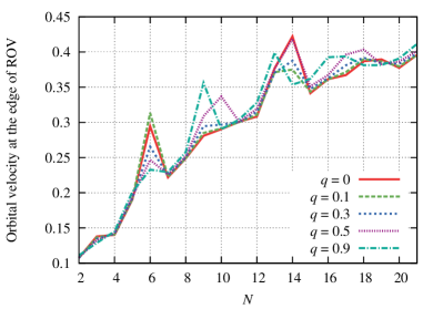
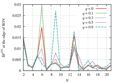
Figure 1: Top: Approximate values of the region of validity (ROV) in the velocity, $\bar{v}^{(N)}$ vs. $N$ for $\delta=0.001$ in the Schwarzschild ($q=a/M=0$) and Kerr ($q=0.1,\,0.3,\,0.5,\,0.9$) cases. Bottom: The relative error evaluated at the edge, $\delta F^{(N)}=|F-F^{(N)}|/F$.

In order to evaluate the above equation, it would be the easiest way to introduce a tolerance. According to Eq. (20) of Ref. Yunes:2008tw ,

$$\Delta^{(N)}_{{\rm ROV}}\equiv\left||F-F^{(N)}|-|F^{(N+1)}-F^{(N)}|\right|<\delta\,,$$ (12)

where $\delta$ is some tolerance, we define the approximate edge of the region of validity.

Since the estimation of the edge depends on the tolerance, an uncertainty width obtained from variations of the tolerance has been shown in Ref. Yunes:2008tw . For simplicity, we focus only on a constant tolerance. In Table 1 and Fig. 1, we present “approximate” values of the edge of the region of validity evaluated from Eq. (12) with $\delta=0.001$ which is the same value used in their paper, for the Schwarzschild ($q=a/M=0$) and Kerr ($q=0.1,\,0.3,\,0.5,\,0.9$) cases. Here, we show the approximate edge of the region of validity in terms of the orbital velocity,

$$v= (M\Omega)^{1/3}\,;$$ (13)

$$\Omega= \frac{M^{1/2}}{r^{3/2}+aM^{1/2}}\,,$$ (14)

and the relative error,

$$\delta F^{(N)}=\frac{|F-F^{(N)}|}{F}\,,$$ (15)

evaluated at the edge. Up to $N=10$ for the Schwarschild case ($q=a/M=0$), this is consistent with Table I of the erratum of Ref. Yunes:2008tw .

It is noted that in the Schwarzschild case the 3PN ($N=6$) order gives the optimal approximation in the analysis up to the 5.5PN order calculation ($N=10$ here). We find a similar feature even in the Kerr cases with small spins ($q=0.1$ and $0.3$) if we consider only the $N=8$ calculations. Although there are various local peaks in Fig. 1, we have larger regions of validity basically if the higher PN results are introduced. In the Kerr case with the spin $q=0.9$, we obtain a large region of validity for $N=9$.

We also note the velocity at the ISCO Bardeen:1972fi which is calculated by substituting Eq. (4) in Eq. (14) as $r=r_{\rm ISCO}$. In practice, the ISCO velocity is derived as $v\approx 0.408248$ ($q=0$), $0.418954$ (0.1), $0.444210$ (0.3), $0.477084$ (0.5), and $0.608618$ (0.9). When we just treat the ISCO velocity as a reference, the edge of the region of validity presented in Fig. 1 does not reach the ISCO velocity for all cases. However, for example, Ref. Fujita:2011zk showed that the 14PN gravitational waveforms can extract an accurate physical information from two-years observation of EMRIs in the Laser Interferometer Space Antenna (LISA) band. Therefore, we need to take account of physical (observational) situations to discuss the practical validity of approximations.

In Ref. Yunes:2008tw , an appropriate tolerance estimation, $\delta_{N}(v)=|F^{(N+2)}(v)-F^{(N+1)}(v)|$ which depends on the PN order, has been introduced because higher-order approximations should be evaluated by an appropriate smaller tolerance. The edge of the region of validity is different from the approximate one obtained in the above. Then, they searched the edge by

$$\Delta^{(N)}_{{\rm ROV}}<\delta_{N}(v)\,.$$ (16)

In the first step, the velocity is set at $v=0.2$, i.e., the tolerance is $|F^{(N+2)}(0.2)-F^{(N+1)}(0.2)|$. By using $\bar{v}^{(N)}$ evaluated by this tolerance, the appropriate tolerance in the next iteration is determined as $|F^{(N+2)}(\bar{v}^{(N)})-F^{(N+1)}(\bar{v}^{(N)})|$. Although we obtain a consistent result with Table II of the erratum of Ref. Yunes:2008tw where they used three successive iterations, we find that there is no appropriate convergent solution for the edge in many iteration. In practice, when we consider $v=0.2$ as the initial guess for the iteration, we have the solution of $\bar{v}^{(N)}\to 0$, or $\bar{v}^{(N)}>v_{\rm ISCO}$ which is beyond our analysis. These behaviors depend on the existence of an intersection of two curves, $\Delta^{(N)}_{{\rm ROV}}$ and $\delta_{N}$ as functions of $v$, and the solutions mean that the inequality of Eq. (16) holds everywhere in the case of $\bar{v}^{(N)}>v_{\rm ISCO}$ for the quasi-circular evolution. Therefore, we do not extend this analysis for higher PN orders here.

III Edges of the allowable region

One of the simplest analysis for the region of validity is to give an allowance $\delta$ for the difference between the numerical (exact) and analytic (PN) results as

$$|F-F^{(N)}|<\delta\,.$$ (17)

In practice, $\delta$ will be numerical accuracies, for example, the allowance of the constraint violations in numerical relativity (NR), and so on. In NR simulations of binary black hole systems Pretorius:2005gq ; Campanelli:2005dd ; Baker:2005vv , the gravitational waveforms are one of the most important output. There are various requirements to obtain the accurate waveforms. One of them is to keep minimizing constraint violations. Since we have discussed the instantaneous valid region at each velocity, this can be considered as the constraint violations of each time slice in the NR simulations .

The error in the PN approximation can be also expressed as the deviation from the “exact” quasi-circular evolution, i.e., the orbital eccentricity, defined by

$$e\equiv \left(\frac{dE}{dr}\right)^{-1}\frac{1}{v}\,F_{\rm Newt}\,|F-F^{(N)}|\,,$$ (18)

where the orbital energy is given by

$$\frac{E}{\mu}= {\frac{{r}^{3/2}-2\,M\sqrt{r}+a\sqrt{M}}{{r}^{3/4}\left({r}^{3/2}-3\,M\sqrt{r}+2\,a\sqrt{M}\right)^{1/2}}}\,,$$ (19)

and we may convert the orbital radius to the velocity as

$$r={\frac{\left[\left(M-{v}^{3}a\right)\sqrt{M}\right]^{2/3}}{{v}^{2}}}\,.$$ (20)

To derive Eq. (18), we convert the energy flux to the radial orbital evolution in quasi-circular inspirals,

$$\frac{dr}{dt}= \left(\frac{dE}{dr}\right)^{-1}\,\frac{dE}{dt}$$ (21)

$$= -\left(\frac{dE}{dr}\right)^{-1}\,F_{\rm Newt}\,F\,.$$ (22)

In the PN approximation, we may use $F^{(N)}$ from Eq. (9), instead of the exact $F$ in the above expression. By analogy to the Newtonian eccentric orbit, the radial trajectory of the orbit with a small eccentricity is written as

$$r(t)\sim r_{0}\left[1-e\cos\left(\frac{vt}{r_{0}}\right)\right]\,.$$ (23)

Here, it is not necessary to treat the difference between the azimuthal and radial frequencies in the Newtonian approximation . In the quasi-circular orbital evolution, the evolution of the radius $r_{0}$ is described by using the exact $F$, and the difference between $F$ and $F^{(N)}$ is related to the eccentricity as

$$\left|\left(\frac{dr}{dt}\right)^{(N)}-\frac{dr}{dt}\right|= \left(\frac{dE}{dr}\right)^{-1}\,F_{\rm Newt}\,|F-F^{(N)}|$$ (24)

$$= ev\sin\left(\frac{vt}{r_{0}}\right)\,,$$ (25)

where we do not consider the oscillation, but treat only the amplitude, i.e., $ev$ in the last equality. Since $v$ in Eq. (18) is a overall factor and we want to just give a rough error estimator, it is sufficient to calculate the eccentricity as the estimator by using the circular orbital velocity $v$ in the azimuthal direction.

Here, as a reference, we simply pick up a number from Table 1 in Ref. Ajith:2012tt . The lowest one is $e\sim 2\times 10^{-5}$ in SpEC SXS_GWD (numerical relativity) waveforms by using an iterative procedure to reduce the eccentricity Boyle:2007ft ; Buonanno:2010yk (see also Refs. Pfeiffer:2007yz ; Purrer:2012wy ). It should be noted that there are various factors to produce the eccentricity in the initial data.

Therefore, for simplicity, we set a restriction on $e$ from the error in the energy flux as

$$e\leq 1\times 10^{-5}\,.$$ (26)

Using this restriction, it is found that the edge of the allowable region is obtained as Fig. 2 in terms of the orbital velocity (top), $v^{(N)}$, and radius (bottom) for the Schwarzschild ($q=0$) and Kerr ($q=0.1,\,0.3,\,0.5,\,0.9$) cases.

In the case of $v<v^{(N)}$, we expect that the PN errors do not influence the eccentricity in the quasi-circular orbital evolution in the current NR simulations. We note that an large edge $v^{(N)}$ is seen for $N=7$, and $N\geq 13$ is required to transcend this value in the Schwarzschild ($q=0$) case. Again, we have larger allowable regions basically if the higher PN results are introduced, although there are various local peaks in Fig. 2. In the bottom panel of Fig. 2, we see that there is a convergent behavior in the orbital radius at $r\sim 8.5M$ in the restriction of $e=1\times 10^{-5}$.

In addition, comparing the top of Fig. 2 to the top of Fig. 1, one can find that the global behaviors of $\bar{v}^{(N)}$ and $v^{(N)}$ are almost same although each value of the velocity or the locations of the local peaks are slightly different. This indicates the global property of the PN convergence.

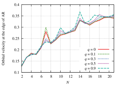
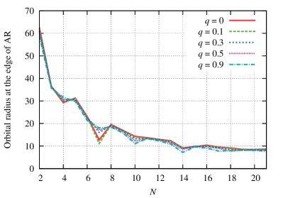
Figure 2: The edge of the allowable region (AR) from the eccentricity estimation in the case of $e\leq 1\times 10^{-5}$ in terms of the orbital velocity (top) and radius (bottom).

IV Discussions

There are various estimates for the region of validity of the PN approximation. For example, the NINJA (Numerical INJection Analysis)-2 project Ajith:2012tt has established that certain 3PN order gravitational waveforms are sufficiently accurate for $v\lesssim 0.33$ to use them as templates for searching gravitational waves from comparable-mass black-hole binaries with the second generation gravitational wave detectors such as Advanced LIGO (aLIGO) TheLIGOScientific:2014jea , Advanced Virgo (AdV) TheVirgo:2014hva , KAGRA Somiya:2011np ; Aso:2013eba , In the NRAR project Hinder:2013oqa , the eccentricity $e\lesssim 0.002$ is one of the requirements for quasi-circular black-hole binaries.

On the other hand, EMRIs treated in this paper are one of the targets for space-based gravitational wave detectors. Although in previous analyses, e.g., Ref. Fujita:2011zk discussed the 14PN gravitational waveforms in the Laser Interferometer Space Antenna (LISA) band, the analysis will be sufficient for a new plan, eLISA Ref. Seoane:2013qna .

In this paper, using the best-known analytic PN and accurate numerical results, 11PN calculation for circular orbits around a Kerr black hole Fujita:2014eta , we revisited the analysis discussed by Yunes and Berti Yunes:2008tw , and obtained the same results in the 5.5PN order calculation for the Schwarschild case. The main results are presented in Table 1 and Fig. 1. In order for the edge of the region of validity to reach the ISCO velocity ($v\approx 0.608618$ for $q=0.9$), much higher PN order calculations will be required. But, this may be just for mathematical interest, and we should discuss gravitational waveforms in practical gravitational wave observations.

Next, we have introduced an eccentricity estimation in Eq. (18) to discuss the allowable region for each PN order, and found that for the small spin cases ($q=0$ and $0.1$) it was difficult to see the improvement due to the use of higher PN order calculations in the previous analysis. This is because the 3.5PN ($N=7$ in Fig. 2) order gives a large allowable region in the $q=0$ and $0.1$ cases and the higher PN calculation than 6.5PN ($N\geq 13$ in Fig. 2) order is required to extend this region. On the other hand, the advantage at $N=7$ is lost in higher spin cases. In terms of the orbital radius, a comparatively smooth expansion of the allowable region can be seen in the higher PN order approximation. Although we have discussed the PN approximation in the case of EMRIs, the higher PN order calculation for comparable-mass binaries would be encouraged.

Here, we note that a reference in Eq. (26) has been assumed to determine the edge of the allowable region for the PN approximation. This means that the edge largely depends on what to discuss. Therefore, it is reasonable to consider the combination of two analyses presented in this paper, i.e., the region of validity and the allowable region. In Fig. 3, we show $\Delta^{(N)}_{{\rm ROV}}$ (defined in Eq. (12)) evaluated at the edge of the allowable region which is obtained in Fig. 2. It is found that only some higher PN order results in the analysis of the edge of the allowable region are valid in the sense of the region of validity if we introduce a constant tolerance. For example, for the higher spinning case ($q=0.9$), we observe that the large allowable region for $N=10$ and $14$ from the eccentricity estimation does not satisfy the constant tolerance $\delta=0.001$ used for the analysis of the region of validity in Sec. II. Therefore, we conclude that any local peak in the top panels of Figs. 1 and 2 does not indicate the best approximation in a given PN order.

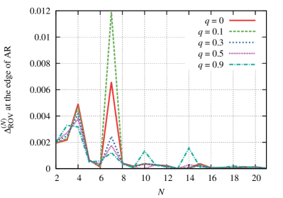
Figure 3: The value of $\Delta^{(N)}_{{\rm ROV}}$ at the edge of the allowable region by using the result shown in Fig. 2.

In this paper, we focus on the PN convergence of the energy flux, which corresponds to the dissipative piece of the self-force under the adiabatic approximation. It is worth considering the PN convergence of the post-adiabatic effects of the self-force, the conservative and the second order dissipative self-forces. In Ref. Isoyama:2012bx , for example, the impact of the post-adiabatic self-force on the gravitational waves has been discussed assuming that the convergence is similar to that of the energy flux. This assumption and their results should be justified when the post-adiabatic self-force is directly calculated.

Finally, we have now various numerical and analytical results for the gravitational radiation reaction in the black hole perturbation approach. For example, Ref. Fujita:2009us discussed a particle moving on eccentric inclined orbits numerically (see also analytical solutions of the bound timelike geodesic orbits in the background Kerr spacetime Fujita:2009bp ). The analytical results have been used to calculate the factorized waveforms Damour:2007xr ; Damour:2008gu which are employed in the effective-one-body approach Buonanno:1998gg (see Refs. Fujita:2010xj ; Pan:2010hz ). Studying region of validity in the PN approximation for these cases is left for future work.

Appendix A From 22PN result for Schwarzschild

From Eq. (5) of Ref. Fujita:2011zk in the PN approximation, the energy flux normalized by the Newtonian flux is written as

$$F^{(N)}=\sum_{k=0}^{N}\sum_{p=0}^{[k/6]}F^{(k,p)}(\ln(v))^{p}v^{k}\,,$$ (27)

where $F^{(0)}=1$, and the normalized “exact” numerical energy flux is denoted by $F$.

In this appendix, we use the 22PN order calculation for circular orbits around a Schwarzschild black hole Fujita:2012cm ; Fujita:2014eta . In Fig. 4, we present $|F^{(k,p)}|$ in Eq. (27) for the cases of $p=0$, $1$ and $2$. Interestingly, the coefficients are approximately fitted by a linear function with respect to $k$ in the log-linear plot. Then, the fitting functions are obtained as

$$F^{(k,0)} = (1.91983)^{k}\,,$$

$$\frac{F^{(k,1)}}{F^{(6,1)}} = (1.96395)^{k-6}\,,$$

$$\frac{F^{(k,2)}}{F^{(12,2)}} = (2.00873)^{k-12}\,.$$ (28)

This fitting means that the radius of convergence for the orbital velocity is derived as

$$v_{R}^{(p=0)} \approx 0.520879\,,$$

$$v_{R}^{(p=1)} \approx 0.509177\,,$$

$$v_{R}^{(p=2)} \approx 0.497828\,,$$ (29)

from the Cauchy ratio test, respectively. These values cover the entire physical domain up to the ISCO velocity, $v_{\rm ISCO}\sim 0.408$.

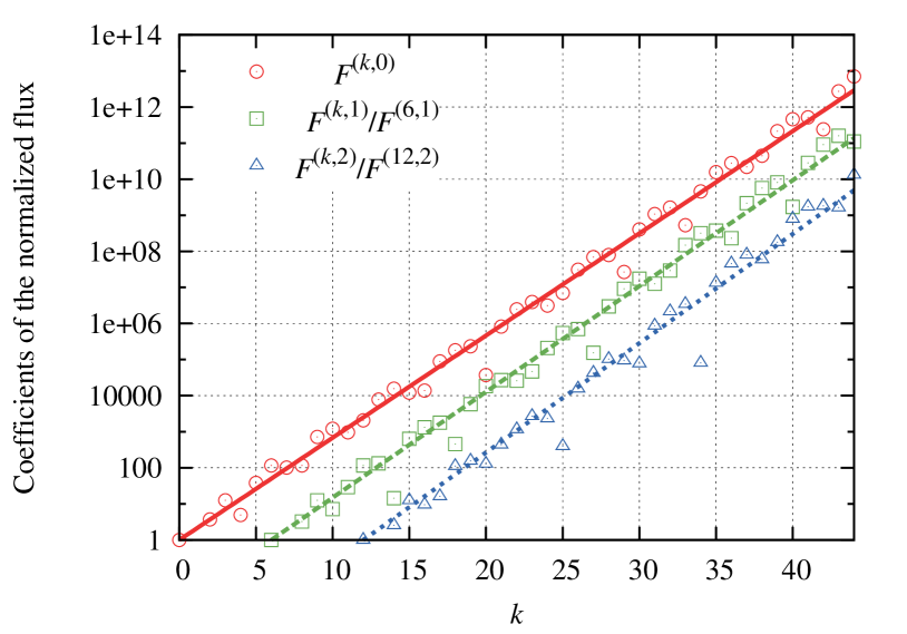
Figure 4: The log-linear plot for the absolute magnitude of some coefficients in Eq. (27) as a function of PN order.

References

- (1) L. Blanchet, Living Rev. Rel. 17, 2 (2014) [arXiv:1310.1528 [gr-qc]].
- (2) M. Sasaki and H. Tagoshi, Living Rev. Rel. 6, 6 (2003) [gr-qc/0306120].
- (3) J. Aasi et al. [LIGO Scientific Collaboration], Class. Quant. Grav. 32, 074001 (2015) [arXiv:1411.4547 [gr-qc]].
- (4) F. Acernese et al. [VIRGO Collaboration], Class. Quant. Grav. 32, 024001 (2015) [arXiv:1408.3978 [gr-qc]].
- (5) K. Somiya [KAGRA Collaboration], Class. Quant. Grav. 29, 124007 (2012) [arXiv:1111.7185 [gr-qc]].
- (6) Y. Aso et al. [KAGRA Collaboration], Phys. Rev. D 88, 043007 (2013) [arXiv:1306.6747 [gr-qc]].
- (7) P. A. Seoane et al. [eLISA Collaboration], arXiv:1305.5720 [astro-ph.CO].
- (8) J. M. Bardeen, W. H. Press and S. A. Teukolsky, Astrophys. J. 178, 347 (1972).
- (9) A. Buonanno and T. Damour, Phys. Rev. D 62, 064015 (2000) doi:10.1103/PhysRevD.62.064015 [gr-qc/0001013].
- (10) A. Ori and K. S. Thorne, Phys. Rev. D 62, 124022 (2000) [gr-qc/0003032].
- (11) M. Kesden, Phys. Rev. D 83, 104011 (2011) [arXiv:1101.3749 [gr-qc]].
- (12) E. Poisson, Phys. Rev. D 52, 5719 (1995) [Addendum-ibid. D 55, 7980 (1997)] [gr-qc/9505030].
- (13) N. Yunes and E. Berti, Phys. Rev. D 77, 124006 (2008) [Erratum-ibid. D 83, 109901 (2011)] [arXiv:0803.1853 [gr-qc]].
- (14) C. M. Bender and S. A. Orszag, Advanced Mathematical Methods for Scientists and Engineers 1, Asymptotic Methods and Perturbation Theory (Springer, New York, 1999).
- (15) Z. Zhang, N. Yunes and E. Berti, Phys. Rev. D 84, 024029 (2011) [arXiv:1103.6041 [gr-qc]].
- (16) R. Fujita, Prog. Theor. Phys. 127, 583 (2012) [arXiv:1104.5615 [gr-qc]].
- (17) T. Tanaka, H. Tagoshi and M. Sasaki, Prog. Theor. Phys. 96, 1087 (1996) [gr-qc/9701050].
- (18) Y. Mino, M. Sasaki, M. Shibata, H. Tagoshi and T. Tanaka, Prog. Theor. Phys. Suppl. 128, 1 (1997) [gr-qc/9712057].
- (19) R. Fujita, Prog. Theor. Phys. 128, 971 (2012) [arXiv:1211.5535 [gr-qc]].
- (20) R. Fujita, PTEP 2015, 033E01 (2015) [arXiv:1412.5689 [gr-qc]].
- (21) N. Sago and R. Fujita, PTEP 2015, 073E03 (2015) [arXiv:1505.01600 [gr-qc]].
- (22) R. Fujita and H. Tagoshi, Prog. Theor. Phys. 112, 415 (2004) [gr-qc/0410018].
- (23) R. Fujita and H. Tagoshi, Prog. Theor. Phys. 113, 1165 (2005) [arXiv:0904.3818 [gr-qc]].
- (24) T. Regge and J. A. Wheeler, Phys. Rev. 108, 1063 (1957).
- (25) F. J. Zerilli, Phys. Rev. D 2, 2141 (1970).
- (26) S. A. Teukolsky, Astrophys. J. 185, 635 (1973).
- (27) E. Newman and R. Penrose, J. Math. Phys. 3, 566 (1962).
- (28) F. Pretorius, Phys. Rev. Lett. 95, 121101 (2005) [gr-qc/0507014].
- (29) M. Campanelli, C. O. Lousto, P. Marronetti and Y. Zlochower, Phys. Rev. Lett. 96, 111101 (2006) [gr-qc/0511048].
- (30) J. G. Baker, J. Centrella, D. I. Choi, M. Koppitz and J. van Meter, Phys. Rev. Lett. 96, 111102 (2006) [gr-qc/0511103].
- (31) P. Ajith, M. Boyle, D. A. Brown, B. Brugmann, L. T. Buchman, L. Cadonati, M. Campanelli and T. Chu et al., arXiv:1201.5319 [gr-qc].
- (32) http://www.black-holes.org/waveforms/
- (33) M. Boyle, D. A. Brown, L. E. Kidder, A. H. Mroue, H. P. Pfeiffer, M. A. Scheel, G. B. Cook and S. A. Teukolsky, Phys. Rev. D 76, 124038 (2007) [arXiv:0710.0158 [gr-qc]].
- (34) A. Buonanno, L. E. Kidder, A. H. Mroue, H. P. Pfeiffer and A. Taracchini, Phys. Rev. D 83, 104034 (2011) [arXiv:1012.1549 [gr-qc]].
- (35) H. P. Pfeiffer, D. A. Brown, L. E. Kidder, L. Lindblom, G. Lovelace and M. A. Scheel, Class. Quant. Grav. 24, S59 (2007) [gr-qc/0702106].
- (36) M. Purrer, S. Husa and M. Hannam, arXiv:1203.4258 [gr-qc].
- (37) I. Hinder et al., Class. Quant. Grav. 31, 025012 (2014) [arXiv:1307.5307 [gr-qc]].
- (38) R. Fujita, W. Hikida and H. Tagoshi, Prog. Theor. Phys. 121, 843 (2009) [arXiv:0904.3810 [gr-qc]].
- (39) R. Fujita and W. Hikida, Class. Quant. Grav. 26, 135002 (2009) [arXiv:0906.1420 [gr-qc]].
- (40) T. Damour and A. Nagar, Phys. Rev. D 76, 064028 (2007) [arXiv:0705.2519 [gr-qc]].
- (41) T. Damour, B. R. Iyer and A. Nagar, Phys. Rev. D 79, 064004 (2009) [arXiv:0811.2069 [gr-qc]].
- (42) A. Buonanno and T. Damour, Phys. Rev. D 59, 084006 (1999) [gr-qc/9811091].
- (43) R. Fujita and B. R. Iyer, Phys. Rev. D 82, 044051 (2010) [arXiv:1005.2266 [gr-qc]].
- (44) Y. Pan, A. Buonanno, R. Fujita, E. Racine and H. Tagoshi, Phys. Rev. D 83, 064003 (2011) [Phys. Rev. D 87, 109901 (2013)] [arXiv:1006.0431 [gr-qc]].
- (45) A. Le Tiec, A. H. Mroue, L. Barack, A. Buonanno, H. P. Pfeiffer, N. Sago and A. Taracchini, Phys. Rev. Lett. 107, 141101 (2011) doi:10.1103/PhysRevLett.107.141101 [arXiv:1106.3278 [gr-qc]].
- (46) S. Isoyama, R. Fujita, N. Sago, H. Tagoshi and T. Tanaka, Phys. Rev. D 87, no. 2, 024010 (2013) doi:10.1103/PhysRevD.87.024010 [arXiv:1210.2569 [gr-qc]].