Dark spherical shell solitons in three-dimensional Bose-Einstein condensates: Existence, stability and dynamics

Abstract

In this work we study spherical shell dark soliton states in three-dimensional atomic Bose-Einstein condensates. Their symmetry is exploited in order to analyze their existence, as well as that of topologically charged variants of the structures, and, importantly, to identify their linear stability Bogolyubov-de Gennes spectrum. We compare our effective 1D spherical and 2D cylindrical computations with the full 3D numerics. An important conclusion is that such spherical shell solitons can be stable sufficiently close to the linear limit of the isotropic condensates considered herein. We have also identified their instabilities leading to the emergence of vortex line and vortex ring cages. In addition, we generalize effective particle pictures of lower dimensional dark solitons and ring dark solitons to the spherical shell solitons concerning their equilibrium radius and effective dynamics around it. In this case too, we favorably compare the resulting predictions such as the shell equilibrium radius, qualitatively and quantitatively, with full numerical solutions in 3D.

I Introduction

The pristine setting of atomic Bose-Einstein condensates (BECs) has offered a significant playground for the examination of numerous physical concepts book1 ; book2 . One of the flourishing directions has been at the interface of the theory of nonlinear waves and such atomic (as well as optical) systems, concerning, in particular, the study of matter-wave solitons emergent ; book_new . Such coherent nonlinear structures have been observed in experiments and studied extensively in theory. Prototypical examples of pertinent studies include —but are not limited to— bright expb1 ; expb2 ; expb3 , dark djf and gap gap matter-wave solitons, as well as vortices fetter1 ; fetter2 , solitonic vortices and vortex rings komineas_rev .

Among these diverse excitations, dark solitons in repulsive BECs have enjoyed a considerable amount of attention in effectively one-dimensional settings due to numerous experiments leading (especially, more recently) to their well-controlled creation chap01:denschl ; chap01:dark1 ; ourmarkus2 ; ourmarkus3 ; seng1 ; seng2 . Moreover, numerous works considered dark solitons in higher-dimensional settings in order to experimentally explore their instability leading to the formation of vortex rings and vortex lines, as illustrated, e.g., in Refs. chap01:dark ; engels ; jeff ; rcg:90 ; pitasv . More recently, such excitations have also been observed in fermionic superfluids martinz ; fprl .

On the other hand, multi-dimensional (i.e., non-planar) variants of dark solitons, were studied as well —cf. e.g., Chapters 7 and 8 of Ref. emergent . Examples of such structures are radially symmetric solitons, such as the ring dark solitons (RDS), initially proposed in atomic BECs in Ref. ring_pap (see also Refs. carrc ; GregHerring ; middel10a for subsequent studies). Nevertheless, such structures were studied to a far lesser extend, arguably due to their generic identified instability, which was found to give rise to states such as alternating charge vortex polygons. Notice that, as was recently shown in Ref. wenlong , stabilization of RDS is possible upon employing a proper potential barrier.

The three-dimensional non-planar generalization of dark solitons, namely spherical shell solitons, has received very limited attention. The analysis of Ref. carrc in the case of box potentials (rather than the typical parabolic trap setting of BECs) revealed their potential existence, but did not pursue their stability analysis. Moreover, the adiabatic dynamics of these structures was studied analytically via a variational approach in Ref. gl without providing, however, relevant numerical results. Nevertheless, it is important to note that in an experimental realization of vortex ring states, the transient observation of spherical shell solitons was reported harvard . In addition, they were also suggested as a potential outcome of collisions of vortex rings in the work of Ref. kominbrand .

It is the purpose of the present manuscript to revisit these states and explore not only their existence in isotropic traps, but also perform their systematic Bogolyubov-de Gennes (BdG) stability analysis. This is done by projecting perturbations onto eigenfunctions of the linear problem in the angular directions. Using this basis, the relevant computations are greatly simplified, and the full 3D spectrum computation is reduced to an effectively small set of one-dimensional problems (for the different modes). It should be mentioned here that the use of spherical harmonics as a basis in the angular variables for states bearing radial symmetry is rather common in terms of numerical schemes for linear and nonlinear Schrödinger (NLS) equations —see, e.g., Ref. hayder for a a recent example. Earlier efforts along these lines in the context of linear Schrödinger equations can be found, e.g., in the works of Refs. herman ; corey . In 2D BECs, analogous decompositions of azimuthal modes for radial states including RDSs and vortices carrc ; GregHerring ; kollar have appeared, and in 3D similar possibilities are starting to emerge wuming .

In this work, we find that indeed spherical shell solitons can be identified as stable 3D solutions of the Gross-Pitaevskii equation, sufficiently close to the linear (small-amplitude) limit of small chemical potential from which they bifurcate, as is shown below. Moreover, we provide a theoretical analysis of their dynamics as “effective particles”. This approach allows to characterize the opposite limit of large chemical potential. Our numerical computations of existence and stability, complemented by direct numerical simulations of the spherical shell soliton dynamics, not only corroborate the above two limits, but also provide a systematic way to interpolate between the two analytically tractable regimes.

Our presentation is organized as follows. First, in Sec. II, we introduce the model and describe the implementation of the linear stability analysis. Our analytical approaches for the spherical shell dark solitons in the above mentioned analytically tractable limits are then presented in Sec. III. Next, in Sec. IV, we present our systematic numerical results. Finally, our conclusions and a number of open problems for future consideration are given in Sec. V. In the Appendix, a similar numerical decomposition method but using cylindrical (rather than spherical) symmetry is also discussed whose results are also given for comparison in Sec. IV.

II Model and Computational Setup

II.1 The Gross-Pitaevskii equation

In the framework of lowest-order mean-field theory, and for sufficiently low-temperatures, the dynamics of a 3D repulsive BEC, confined in a time-independent trap $V$, is described by the following dimensionless Gross-Pitaevskii equation (GPE) book1 ; book2 ; emergent ; book_new :

$$i\psi_{t}=-\frac{1}{2}\nabla^{2}\psi+V\psi+|\psi|^{2}\psi-\mu\psi,$$ (1)

where $\psi(x,y,z,t)$ is the macroscopic wavefunction of the BEC and $\mu$ is the chemical potential (subscripts denote partial derivatives). Here, we consider a harmonic trap of the form:

$$V=\frac{1}{2}\omega_{\rho}^{2}\rho^{2}+\frac{1}{2}\omega_{z}^{2}z^{2},$$ (2)

where $\rho=\sqrt{x^{2}+y^{2}}$, $\omega_{\rho}$ and $\omega_{z}$ are the trapping frequencies along the $(x,y)$ plane and the vertical direction $z$, respectively. Note that the potential has rotational symmetry with respect to the $z$-axis. In our numerical simulations, we focus on the fully symmetric (isotropic, spherically symmetric) case with $\omega=\omega_{\rho}=\omega_{z}=1$, in which we can benchmark our numerical methods in effective 1D and 2D against those of the fully 3D setting.

We examine the dark spherical shell solitons, hereafter referred to as DSS. This single radial node state exists in this isotropic case from the linear limit onwards as a stationary state of the form $\psi(x,y,z,t)=e^{-i\mu t}\psi_{\rm{DSS}}(r)$ where $r=\sqrt{x^{2}+y^{2}+z^{2}}$ is the spherical radial variable. At the linear limit, the waveform is an eigenmode of the quantum harmonic oscillator with chemical potential $\mu=7\omega/2$, and spatial profile:

$$|\psi_{\rm{DSS}}\rangle_{\rm{linear}} = \frac{1}{\sqrt{3}}\left(|200\rangle+|020\rangle+|002\rangle\right)$$ (3)

$$\propto \left(\omega r^{2}-\frac{3}{2}\right)e^{-\omega r^{2}/2},$$ (4)

where the basis $\{|n_{x}n_{y}n_{z}\rangle\}$ denotes the 3D harmonic oscillator quantum states in Cartesian coordinates.

The DSS is generally expected to be unstable for high chemical potentials due to transverse modulational (snaking-type) instability, in a way similar to its planar and RDS counterparts, as summarized, e.g., in Refs. book_new ; djf . However, for smaller chemical potentials, and especially near the linear limit, it is relevant to analyze stability of the DSS and identify corresponding instabilities and where they may arise. In what follows (cf. Sec. IV below), we will turn to numerical computations, based on a fixed point iteration and our spherical harmonic decomposition of the spectral stability BdG problem, in order to efficiently identify the intervals of existence and stability of the relevant modes.

II.2 The Linear Stability Problem: Spherical Harmonic Decomposition

In this section, we discuss our analysis of the linear stability of the DSS states utilizing their effective 1D nature, namely their spherical symmetry. In spherical coordinates $(r,\theta,\phi)$, the Laplacian can be decomposed into radial and angular parts, denoted by $\Delta_{R}$ and $\Delta_{S}$ respectively, namely

$$\nabla^{2}f=\Delta_{R}f+\frac{\Delta_{S}f}{r^{2}},$$ (5)

where

$$\Delta_{R}f = \frac{1}{r^{2}}\frac{\partial}{\partial r}\left(r^{2}\frac{\partial f}{\partial r}\right),$$ (6)

$$\Delta_{S}f = \frac{1}{\sin\theta}\frac{\partial}{\partial\theta}\left(\sin\theta\frac{\partial f}{\partial\theta}\right)+\frac{1}{\sin^{2}\theta}\frac{\partial^{2}f}{\partial\phi^{2}},$$ (7)

The $\Delta_{S}$ operator has eigenstates given by the spherical harmonics $\{Y_{\ell m}\}$ with eigenvalues $-\ell(\ell+1)$, i.e.,

$$\Delta_{S}Y_{\ell m}=-\ell(\ell+1)Y_{\ell m}.$$ (8)

For states with spherical symmetry ($\ell=0$), the $\Delta_{S}$ part of the Laplacian is not relevant for identifying the stationary state. Thus, the stationary DSS state $\psi_{0}(r)$ of Eq. (1), defined in the domain $r\in[0,\infty)$, satisfies the following radial equation:

$$-\frac{1}{2}\Delta_{R}\psi_{0}+V(r)\psi_{0}+|\psi_{0}|^{2}\psi_{0}-\mu\psi_{0}=0.$$ (9)

Now, let us consider the linear stability (BdG) spectrum of such a stationary state. We consider small-amplitude perturbations expanded using the complete basis of $\{Y_{\ell m}\}$ (the spherical harmonic eigen-basis) as follows:

$$\psi(r,t)=\psi_{0}+\sum\limits_{\ell m}\left[a_{\ell m}(r,t)Y_{\ell m}+b_{\ell m}^{*}(r,t)Y_{\ell m}^{*}\right],$$ (10)

where the space- and time-dependent coefficients $a_{\ell m}(r,t)$ and $b_{\ell m}(r,t)$ determine the radial and temporal evolution of the perturbation. Then, substituting Eq. (10) into Eq. (1) and retaining up to linear terms in the expansion, one notes that all the $\ell$ modes are mutually independent due to the spherical symmetry of the steady state. For mode $\ell$, the coefficients $a$ and $b$ of the expansion obey the following evolution equations:

$$\begin{array}[]{rcl}ia_{t}&=&-\frac{1}{2}\Delta_{R}a+\frac{\ell(\ell+1)}{2r^{2}}a+Va+2|\psi_{0}|^{2}a+\psi_{0}^{2}b-\mu a,\\[4.30554pt] -ib_{t}&=&-\frac{1}{2}\Delta_{R}b+\frac{\ell(\ell+1)}{2r^{2}}b+Vb+2|\psi_{0}|^{2}b+\psi_{0}^{*2}a-\mu b,\end{array}$$

where we have dropped for simplicity the subscripts $(\ell,m)$. As we are interested in the stability of the steady-state, we now expand the coefficients using

$$\begin{pmatrix}a\\ b\end{pmatrix}=\begin{pmatrix}a_{0}\\ b_{0}\end{pmatrix}e^{\lambda t},$$ (11)

where $\lambda$ is an eigenvalue of the following matrix

$$M=\begin{pmatrix}M_{11}&M_{12}\\ M_{21}&M_{22}\end{pmatrix},$$ (12)

with

$$\begin{array}[]{rcl}M_{11}&=&-i\left(-\frac{1}{2}\Delta_{R}+\frac{\ell(\ell+1)}{2r^{2}}+V+2|\psi_{0}|^{2}-\mu\right),\\[8.61108pt] M_{12}&=&-i\psi_{0}^{2},\\[4.30554pt] M_{21}&=&i\psi_{0}^{*2},\\[4.30554pt] M_{22}&=&i\left(-\frac{1}{2}\Delta_{R}+\frac{\ell(\ell+1)}{2r^{2}}+V+2|\psi_{0}|^{2}-\mu\right).\end{array}$$

One can, therefore, compute the full spectrum by computing that of each mode $\ell$ independently, and then putting them all together to “reconstruct” the full spectrum. In what follows we use $\ell=0,1,2,...,10$ for values of the chemical potential up to $\mu\approx 12$. The reduction of dimensionality with the decomposition on a complete basis set is also available in 2D for states with rotational symmetry up to a topological charge along the $z$ axis. For clarity, this is shown in the Appendix. It is worth mentioning that a large class of BEC states belongs to this class.

Finally, we discuss the application of the degenerate perturbation method (DPM) ourVRfromLinear to the DSS state. This method is employed for the determination of the DSS’ spectrum near the linear limit, and also for the identification of the nature of instabilities. The method can be most readily understood from the 3D version of the matrix $M$, where one can separate the free (linear) part with known eigenstates and eigenvalues and the rest of the terms can be treated as perturbations near the linear limit. Note that there are 2$\times$2 block matrices within $M$ and the complete basis consists of both “positive” and “negative” eigenstates. This terminology is associated with quantum harmonic oscillator eigenstates leading to positive or negative eigenvalues for the linear analogs of the operators $M_{ii}$ in Eq. (12) i.e., with $|\psi_{0}|^{2}$ set to $0$. In DPM, the functional dependence of the eigenvalues on the chemical potential $\mu$ is dominated by the interplay of equi-energetic, degenerate states. The result of the nonlinear perturbations ($\propto|\psi_{0}|^{2}$) in $M_{ij}$ within Eq. (12) is to cause the degenerate eigenvalues to depart from their respective linear limit, as the norm of the solution (mass) increases. The free part provides the basis that is formed from “up” states and “down” states, of the form $\begin{pmatrix}|n_{x}n_{y}n_{z}\rangle\\ 0\end{pmatrix}$ and $\begin{pmatrix}0\\ |n_{x}n_{y}n_{z}\rangle\end{pmatrix},$ with eigenvalues $E_{|n_{x}n_{y}n_{z}\rangle}-E_{\rm{DSS}}$ and $E_{\rm{DSS}}-E_{|n_{x}n_{y}n_{z}\rangle}$ respectively, where $E_{\Lambda}$ is the eigenenergy of the 3D quantum harmonic oscillator for eigenstate $\Lambda$. The relevant states for eigenvalues near the spectrum of Im($\lambda$)=0, 1 and 2 are listed in Table. 1. Then, the effect of the nonlinearity on these eigenmodes and the corresponding eigenvalue corrections are calculated, as discussed in Ref. ourVRfromLinear (and originally spearheaded in this context in Ref. feder ). Below, this is compared to the numerical spectrum in Sec. IV.

Table 1: Relevant states for eigenvalues near the spectrum of Im($\lambda$)=0,1 and 2 for the degenerate perturbation theory. Here $|m\,n\,p\rangle$ stands for eigenstates with all possible distinct permutations with the quantum numbers $m,n$ and $p$.

Im($\lambda$)	“up” states	“down” states
$0$	$|002\rangle$ $|011\rangle$	$|002\rangle$ $|011\rangle$
$1$	$|003\rangle$ $|012\rangle$ $|111\rangle$	$|001\rangle$
$2$	$|004\rangle$ $|013\rangle$ $|022\rangle$ $|112\rangle$	$|000\rangle$

III The particle picture for the DSS

We now turn to the limit of large chemical potential $\mu$. In this so-called Thomas-Fermi (TF) limit of large $\mu$, the ground state of the GPE is approximated as $\psi_{\rm{TF}}=\sqrt{\max(\mu-V,0)}$ book1 ; book2 . A natural way to obtain a reduced dynamical description of the DSS —analogously to what is done in lower-dimensional settings— is to develop an effective particle picture for the DSS in the TF limit. Here, following Ref. wenlong , we focus on the equilibrium radius $r_{c}$ of the DSS, as a prototypical diagnostic that we can compare to our numerical results. This equilibrium radius is determined as the critical value of the DSS radius for which the restoring force due to the harmonic trap is counterbalanced by the effective force exerted due to the curvature of the DSS.

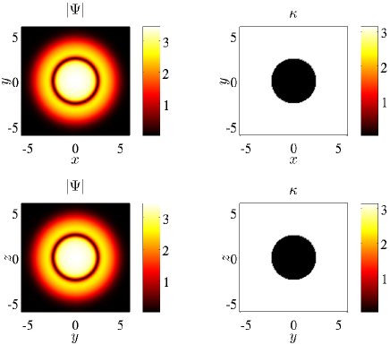
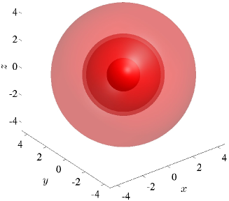
Figure 1: (color online) The two pairs of the top panels show the modulus $|\Psi|$ (left panels) and argument $\kappa$ (right panels) of a dark soliton shell state at $\mu=12$; the top row illustrates the $z=0$ plane, while the middle row the $x=0$ plane. The bottom panel shows an isocontour plot of the same state.

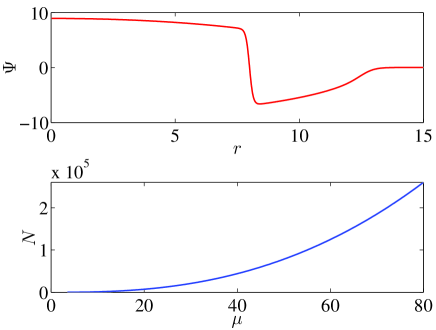
Figure 2: (Color online) Top panel: a radial profile of the dark soliton shell state in the TF limit for $\mu=80$. Bottom panel: number of particles as a function of chemical potential $\mu$, showing the continuation of states from the linear limit to the nonlinear regime.

The first approach (motivated also by the work of Ref. kapermorg ) focuses on the stationary state using the ansatz $\psi(r)=\psi_{\rm TF}(r)q(r)$, where one obtains an equation for the DSS profile $q(r)$ (on top of the TF ground-state $\psi_{\rm TF}$) given by:

$$\frac{1}{2}q^{\prime\prime}+\mu q(1-q^{2})=P(r),$$ (13)

where

$$P(r)=Vq(1-q^{2})-\frac{2}{r}q^{\prime}-\frac{\psi_{\rm TF}^{\prime\prime}}{2\psi_{\rm TF}}q-\frac{\psi_{\rm TF}^{\prime}}{\psi_{\rm TF}}q^{\prime}-\frac{1}{r}\frac{\psi_{\rm TF}^{\prime}}{\psi_{\rm TF}}q,$$

and primes denote derivatives with respect to $r$. Inspired by the profile of the 1D and 2D equivalents of the DSS, namely the dark soliton and the RDS, we seek a stationary DSS solution in the form of $q(r)=\tanh[\sqrt{\mu}(r-r_{c})]$. Multiplying both sides of Eq. (13) by $q^{\prime}$ and integrating over $r$ from $-\infty$ to $\infty$ (bearing in mind that the contribution of the integral from $r=-\infty$ to $r=0$ is exponentially small), we find that the equilibrium radius is given by

$$r_{c}=\frac{\sqrt{\alpha\mu}}{\omega},$$ (14)

where $\alpha=5-\sqrt{17}\approx 0.8769$. This result, as in the case of the dark soliton ring in 2D wenlong , slightly overestimates the actual value for $\alpha$ that, as we will see below, is accurately predicted by the second particle picture approach, which retrieves the precise value for $\alpha$ to be $\alpha=4/5$; this is confirmed by the numerical results shown below, in Sec. IV.

The second approach relies on energy conservation and it is based on the analysis of Ref. kamch . In this approach, it is argued that the equation of motion can be derived by a local conservation law (i.e., an adiabatic invariant) in the form of the energy of a dark soliton under the effect of curvature and of the density variation associated with it. More specifically, knowing that the energy of the 1D dark soliton centered at $x_{c}$ is given by ${\cal E}=(4/3)(\mu-\dot{x}_{c})^{3/2}$ djf , the generalization of the relevant adiabatic invariant quantity in a 3D domain bearing density modulations reads:

$$\begin{array}[]{rcl}{\cal E}&=&4\pi r^{2}\left[\frac{4}{3}(\mu-V(r)-\dot{r}^{2})^{3/2}\right]\\[4.30554pt] &=&4\pi r_{0}^{2}\left[\frac{4}{3}(\mu-V(r_{0})-\dot{r}_{0}^{2})^{3/2}\right],\end{array}$$ (15)

where $r(t)$ and $\dot{r}(t)$ are the (radial) location and velocity of the DSS with initial conditions $r_{0}$ and $\dot{r}_{0}$. Taking a time derivative on both sides of Eq. (15) and assuming that the DSS has no initial speed ($\dot{r}_{0}=0$), we obtain a Newtonian particle equation of motion for the DSS of the following form:

$$\ddot{r}=-\frac{1}{2}\frac{\partial V}{\partial r}+\frac{2}{3r}\left(\frac{r_{0}}{r}\right)^{4/3}[\mu-V(r_{0})].$$ (16)

From this equation, the equilibrium position for the DSS yields $r_{c}=\sqrt{\dfrac{4\mu}{5}}/\omega$, a result consistent with the numerical findings of the next Section. We now proceed to test these predictions, the stability analysis spectrum, and the equilibrium positions for the DSS.

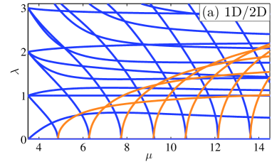
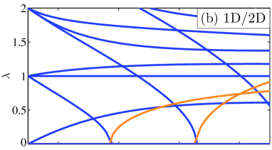
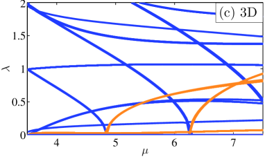
Figure 3: (Color online) Stability spectra for the dark soliton shell as a function of the chemical potential $\mu$. (a)-(b) Spectra computed using our effectively 1D method (in the radial variable, using a spherical harmonic decomposition in the transverse directions). Identical results are obtained when using the 2D variant of the method in cylindrical coordinates (and decomposing only the azimuthal direction in suitable Fourier modes). Both 1D and 2D numerics use a spacing of $h=0.01$. (c) Spectra computed using the full 3D numerics with spacing $h=0.2$. Orange (grey) lines depict the real part of $\lambda$ (i.e., unstable parts of the eigenvalues), while blue (dark) lines the imaginary part of $\lambda$.

IV Numerical vs. analytical results

Let us start by providing some of the basic features of the DSS. A typical DSS state at $\mu=12$ is shown in Fig. 1, where its spherical symmetry is apparent. A radial plot of the wavefunction in the TF limit is depicted in the top panel of Fig. 2. As the chemical potential is increased the number of atoms (“mass”)

$$N=\int|\psi|^{2}dxdydz=4\pi\int_{0}^{\infty}r^{2}|\psi|^{2}dr,$$ (17)

increases as depicted in the bottom panel of Fig. 2.

We now examine the stability of the DSS. The corresponding spectra illustrating the imaginary part of the eigenvalues [dark (blue) lines) and the real part [light (orange) lines] are shown in Fig. 3. Panel (a) depicts the spectrum obtained via our numerical method over a wide range of chemical potentials. Identical results were obtained when using the method in 2D, based on a cylindrical coordinate decomposition and a representation of the azimuthal variable dependence in the corresponding Fourier modes. For reasons of completeness, a summary of this variant of the method is presented in the appendix. Panels (b) and (c) depict a zoomed in region to contrast the results between these lower dimensional methods and the full 3D numerics. Panel (b) corresponds to the spectrum as computed by means of the 1D spherical coordinate decomposition method using spherical harmonics with spatial spacing of $h=0.01$, while panel (c) depicts the results from direct full 3D numerics using an spatial spacing of $h=0.2$. A close comparison between the panels suggests small discrepancies of the imaginary parts at Im$(\lambda)=1$ and Im$(\lambda)\approx 0.2$, and a spurious unstable mode with Re$(\lambda)\approx 0.08$. These discrepancies (and their amendment as the mesh resolution $h$ decreases —see below) are likely due to the large spatial spacing $h$ —that needs to be chosen such that the 3D calculations are still “manageable”— in which case the DSS radial profile is under-resolved. It is crucial to note that the 3D calculations are far more expensive than their lower dimensional (1D or 2D) counterparts considered above.

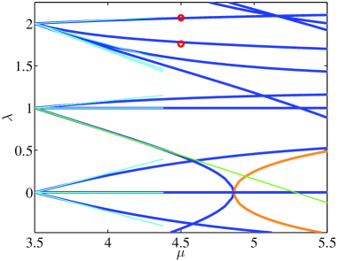
Figure 4: (Color online) Comparison near the linear limit of the spectrum of the degenerate perturbation method and the numerical result of the effectively 1D method involving the spherical harmonic decomposition. Thick blue (dark) and orange (light) lines depict the imaginary and real parts of the numerical eigenvalues while the thinner cyan and green lines depict the theoretical results of the degenerate perturbation method. The eigenvalue depicted in green is the one responsible for the destabilization of the DSS. The large red dots correspond to the two frequencies extracted from the oscillations of the perturbed DSS depicted in Fig. 5. The larger frequency corresponds to the oscillatory mode of the DSS while the smaller one corresponds to the breathing mode of the background density.

To confirm that the discrepancies are indeed caused by the mesh resolution, when we further decrease the lattice spacing to $h=0.15$ (results not shown here) and recalculate the spectrum in 3D, the branches at Im$(\lambda)=1$ indeed split into two non-degenerate curves and the spurious modes at Im$(\lambda)\approx 0.2$ and Re$(\lambda)\approx 0.08$ begin to get suppressed. This suggests that the discrepancies are indeed attributable to resolution effects and that the spectrum computed with the effectively 1D numerical method is indeed accurate.

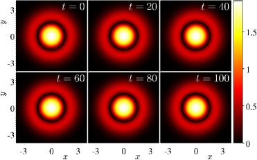
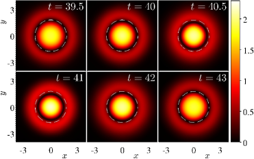
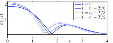
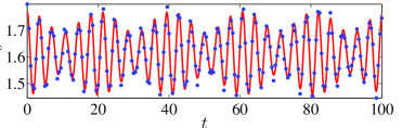
Figure 5: (Color online) Top set of panels: 2D density cuts ($z=0$) from the full 3D numerical solution for $\mu=4.5$. The initial condition corresponds to the stationary DSS at its equilibrium radius. Second set of panels: Evolution of a DSS shifted from its equilibrium position undergoing oscillatory motion over one oscillation period $T$. The white dashed circle denotes the starting location of the DSS at the beginning of the period. Third panel: Radial profiles for the oscillating DSS over half a period. Bottom panel: Oscillations of the DSS radius vs. time. Blue dots represent the radius extracted from full 3D numerics while the solid red line is the best (least-square) fit to a linear combination of oscillations with frequencies $w_{1}\approx 1.7581$ and $w_{2}=2.0671$ (see red dots in Fig. 4) corresponding, respectively, to the frequencies of the DSS oscillations and the breathing mode of the background cloud. For a movie depicting the stable oscillations of the DSS please see the supplemental material.

The comparison between the stability spectrum predicted by the degenerate perturbation method (DPM) and the one obtained numerically near the linear limit is shown in Fig. 4. As the figure shows, the DPM captures the behavior of the spectrum close to the linear limit. Let us now confirm the stability of the DSS in this limit. We have performed a direct numerical integration of the full 3D dynamics of the DSS for $\mu=4.5$, where it is predicted to be stable —cf. Figs. 3 and 4. This evolution is depicted in the top set of panels of Fig. 5. Also, in this figure, we depict the stable oscillations of a perturbed DSS by displacing its initial location away from the equilibrium radius. The evolution for such a DSS performing oscillations is displayed in the second set of panels in Fig. 5. A movie for this evolution is provided in the supplemental material. To more clearly visualize these oscillations, we depict on the third panel of Fig. 5 the transverse density cuts at four different stages over half a period of the oscillation. These density cuts also reveal the excitation of the background cloud which performs breathing oscillations. From the density cuts we extracted the (radial) location of the DSS along the evolution which displays a beating-type quasiperiodic oscillation as depicted by the blue dots in the bottom panel of Fig. 5. In fact, by (least-square) fitting a linear combination of two harmonic oscillations (see red line) we extract the frequencies $w_{1}\approx 1.7581$ and $w_{2}=2.0671$. Upon closer inspection, these frequencies correspond, respectively, to the frequency of the DSS oscillations and the frequency of the breathing mode of the background cloud. These frequencies are also depicted in Fig. 4 clearly showing that they indeed belong to the stability spectrum of the stationary DSS state. It is important to stress that the observed DSS oscillations are supported by the stability of the DSS at its equilibrium position. Therefore, despite strong perturbations of the background that undergoes breathing oscillations, the DSS robustly persists and performs stable oscillations about its equilibrium position.

As the spectrum indicates, see Figs. 3 and 4, for larger values of the chemical potential the DSS becomes unstable. To identify this instability, we have looked at the eigenvectors of the DPM. There are high degeneracies in the eigenvalues in this case, rendering harder the identification of the nature of the instability. Nevertheless, the DPM is still helpful in that regard. For instance, we know from the eigenvectors that the mode with the largest slope decreasing at Im$(\lambda)=1$, which causes instabilities, is a linear combination of “up” states, and the “down” states are not involved. Therefore, the instability is due to a bifurcation rather than a collision with “negative” energy modes; the latter may lead to oscillatory instabilities, as discussed, e.g., in Ref. ourVRfromLinear . The former may be associated with symmetry breaking features and exhibits the instability via real eigenvalue pairs. Direct numerical integration of Eq. (1) for chemical potentials $\mu=5.8,8.2$ and 10.6, shows that the first instability is a bifurcation of a six vortex lines (VL6) cage, while the rest of the instabilities are dominated by a cubic six vortex rings (VR6) cage. The first instability suggests a bifurcation of VL6 from the interactions of the DSS and a dark soliton state with three plane nodes perpendicular to the $(x,y)$-plane, separated by angles of $\pi/3$; the dark soliton state (DS3) can be written as

$$|\psi_{\rm{DSm}}\rangle_{\rm{linear}} \propto \rho^{m}\cos(m\phi)e^{-\omega r^{2}/2},$$ (18)

with $m=3$ and a linear eigenenergy $(m+\frac{3}{2})\omega$. A two-mode analysis theochar ; ourVRfromLinear using this state and the DSS state yields a prediction of the bifurcation as occurring at $\mu_{c}=4.78$, which is in good agreement with the numerical result $\mu_{c}=4.85\pm 0.01$ of Fig. 3. A similar treatment of the VR6 cage turns out to be more challenging due to the difficulty in designing the corresponding dark soliton state. Instead, we have looked at the DS4 state, which can form an eight vortex line (VL8) cage. The two-mode analysis then predicts a bifurcation at $\mu_{c}=5.97$, which is in fair agreement with the second instability at $\mu_{c}=6.25\pm 0.01$ from Fig. 3. The numerical results, however, show that the dynamically resulting state is a VR6 cage, not a VL8 cage. Presumably the VL8 cage can also cause instabilities of the DSS but is less robust than the VR6 cage, possibly due to the intersections of the vortex lines, which are absent in VR6. Further analysis with higher values of $m$ (not shown here) also suggests the progressively lesser relevance of the DSm state in causing instabilities. On the other hand, the VR6 state seems to be very robust and dominates the instability in a wide range of chemical potentials from the onset of this instability around $\mu=6.2$. The VL6 and VR6 cages are shown in Fig. 6.

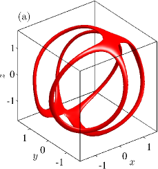
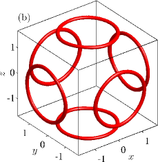
Figure 6: (Color online) The VL6 cage (a) and the VR6 cage (b) that emerge as a result of the instability of the DSS state. The states are captured from the numerical integration of the GPE (1) dynamics at $\mu=5.8$ and $8.2$, respectively. In particular, the VR6 cage seems to be robust and appears in the dynamics for a wide range of chemical potentials from the onset of the instability around $\mu=6.2$.

Finally, we present the numerical results for the equilibrium location $r_{c}$ of the DSS as a function of the chemical potential $\mu$ and compare the results with those of the two particle pictures in the large density limit (see Sec. III). A plot of $r_{c}\omega/\sqrt{\mu}$ as a function of $\mu$ is depicted in Fig. 7. Note that the first particle picture predicts a slightly larger equilibrium $r_{c}$, while the particle picture based on energy conservation of the DSS as an adiabatic invariant agrees very well with the numerical results. It is interesting to note that the asymptotic behavior only sets in at about $\mu=30$, deep inside the TF regime. Although this would be a rather computationally demanding parametric range when using 3D (or even 2D) methods, our effective 1D approach based on a spherical harmonic decomposition of the angular dependencies, allows us to reach such large values of $\mu$.

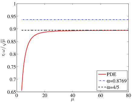
Figure 7: (Color online) The equilibrium radius of the spherical shell dark soliton, scaled by $\sqrt{\mu}/\omega$, as a function of $\mu$ (solid red line). Note that the numerical values reach the asymptotic value of $\sqrt{4/5}$ (dashed black line), as per the second particle picture, when $\mu$ is large. The first particle picture slightly overestimates $r_{c}$ (dash-dotted blue line).

V Conclusions and Future Challenges

In this work, we have revisited the theme of spherical shell dark solitons. We have employed analytical methods to study these structures both in the vicinity of the linear limit, using a bifurcation analysis, and in the Thomas-Fermi limit, where they can be treated as effective particles. For the numerical simulations, we have used continuation methods, as well as a quasi-one-dimensional radial computation method, decomposing the angular dependence of the perturbations in spherical harmonics, to determine their stability. We have found that spherical shell dark solitons can, in fact, be dynamically robust, spectrally stable solutions of the 3D Gross-Pitaevskii equation within a certain interval of chemical potentials (and atom numbers); this occurs sufficiently close to the linear limit of relatively small chemical potentials. Their instabilities, emerging when the chemical potential increases, have been elucidated and their dynamical outcome, namely the breakup into vortex ring and vortex line cages, has been showcased. We believe that these results, may not only be used to partially explain the transient observation of these structures in earlier experiments harvard and numerical simulations kominbrand , but may also pave the way for their consideration in future experiments.

Our work suggests a number of interesting future research directions, concerning, in particular, related coherent structures, their physical relevance and properties. For instance, this study suggests large scale stability computations for a wide range of pertinent steady states with radial symmetry, including ones with different numbers of radial nodes as well as a number of different external potentials. Furthermore, it would be relevant to generalize and apply the numerical (and analytical) techniques used herein to multicomponent BEC settings. For example, one can study “symbiotic states” composed of spherical shell dark-bright solitons, in the spirit of the dark-bright 2D rings of Ref. stockhofe . On the other hand, states emerging robustly from the instabilities of these spherically (or cylindrically) symmetric ones, such as the vortex ring (and line) cages are worthwhile to investigate further in their own right. Efforts along these directions are currently in progress and will be presented in future publications.

APPENDIX: 2D DECOMPOSITION USING CYLINDRICAL COORDINATES

The greatest advantage of the 1D method involving the decomposition into spherical harmonics is that one can compute the spectrum for large chemical potentials without excessive computational costs. The reason that typical computations for large chemical potentials become computationally prohibitive, is that in this limit the density is large and, thus, the width of the relevant localized structures (proportional to $1/\sqrt{\mu}$) becomes much smaller than the domain size (proportional to $\sqrt{\mu}$); hence, a large number of mesh points is necessary to resolve properly these configurations. Nonetheless, it is worth mentioning that, for the projection method in 1D, the form of states that one can study is also restricted by the spherical symmetry; therefore, it is also relevant to employ an analog of this method in 2D, so as to encompass a wider class of states. An example concerns states with a topological charge $S$ along the $z$ axis, i.e., stationary states of the form $\psi=\psi_{0}\,e^{iS\phi}$. Note that in this framework, one can study states including —but not limited to— the ground-state, planar, ring, or spherical shell dark soliton states, vortex lines, as well as coplanar or parallel vortex rings and hopfions hopfion , in both isotropic and anisotropic traps.

In 2D, and for cylindrical coordinates $(\rho,\phi,z)$, the Laplacian is decomposed as follows:

$$\nabla^{2}f=\Delta_{H}f+\frac{\Delta_{G}f}{\rho^{2}},$$ (19)

where its components read:

$$\Delta_{H}f = \frac{1}{\rho}\frac{\partial}{\partial\rho}\left(\rho\frac{\partial f}{\partial\rho}\right)+\frac{\partial^{2}f}{\partial z^{2}},$$ (20)

$$\Delta_{G}f = \frac{\partial^{2}f}{\partial\phi^{2}}.$$ (21)

The $\Delta_{G}$ operator has eigenstates $\{e^{im\phi}\}$ with eigenvalues $-m^{2}$, i.e.,

$$\Delta_{G}e^{im\phi}=-m^{2}e^{im\phi}.$$ (22)

A stationary state $\psi_{0}(\rho,z)$, defined in the domain $\rho\in[0,\infty)\times z\in\mathbb{R}$, and bearing a topological charge $S$, satisfies the following equation:

$$-\frac{1}{2}\Delta_{H}\psi_{0}+\frac{S^{2}}{2\rho^{2}}\psi_{0}+V(\rho,z)\psi_{0}+|\psi_{0}|^{2}\psi_{0}-\mu\psi_{0}=0,$$ (23)

As in the 1D case, we construct the linear stability problem as follows. Let $\psi_{0}$ a rotationally symmetric stationary state, up to a topological charge $S$, along the $z$ axis perturbed using the complete basis of $\{e^{im\phi}\}$:

$$\psi=e^{iS\phi}\left[\psi_{0}+\sum\limits_{m}\left[a_{m}(\rho,z,t)e^{im\phi}+b_{m}^{*}(\rho,z,t)e^{-im\phi}\right]\right].$$

Substituting this expansion into the GPE of Eq. (1), and upon linearizing and matching the basis expansion on both sides, one can see that the different $m$ modes are mutually independent. An equivalent derivation as in 1D shows that $\lambda$ are the eigenvalues of the matrix

$$M=\begin{pmatrix}M_{11}&M_{12}\\ M_{21}&M_{22}\end{pmatrix},$$

where

$$\begin{array}[]{rcl}M_{11}&=&-i\left(-\frac{1}{2}\Delta_{H}+\frac{(m+S)^{2}}{2\rho^{2}}+V+2|\psi_{0}|^{2}-\mu\right),\\[8.61108pt] M_{12}&=&-i\psi_{0}^{2},\\[4.30554pt] M_{21}&=&i\psi_{0}^{*2},\\[4.30554pt] M_{22}&=&i\left(-\frac{1}{2}\Delta_{H}+\frac{(m-S)^{2}}{2\rho^{2}}+V+2|\psi_{0}|^{2}-\mu\right).\end{array}$$

As before, one can therefore compute the full spectrum by computing each mode $m$ independently and then putting them together. In the results based on this method and presented in Sec. IV, we use $m=0,1,2,...,5$. It is worth commenting here that the matrix for the 2D eigenvalue problem with a charge $S$ is less symmetric than matrices corresponding to the 1D projection and the 2D case with no charge. Therefore, the full 2D problem with charge appears to demand more computational work. However, it should be noted that, in the 2D case, the eigenvalues of the full matrix $M$ corresponding to the projections over the $+m$ and $-m$ modes are related via an orthogonal transformation and, thus, the two set of eigenvalues are complex conjugates of each other. Therefore, it is only necessary to compute the non-negative $m$ set and, hence, the charged and the uncharged states actually have similar computational complexity.

References

- (1) C. J. Pethick and H. Smith, Bose-Einstein Condensation in Dilute Gases (Cambridge University Press, Cambridge, 2008).
- (2) L. P. Pitaevskii and S. Stringari, Bose-Einstein Condensation (Oxford University Press, Oxford, 2003).
- (3) P. G. Kevrekidis, D. J. Frantzeskakis, and R. Carretero-González (eds.), Emergent Nonlinear Phenomena in Bose-Einstein Condensates. Theory and Experiment (Springer-Verlag, Berlin, 2008); R. Carretero-González, D. J. Frantzeskakis, and P. G. Kevrekidis, Nonlinearity 21, R139 (2008).
- (4) P. G. Kevrekidis, D. J. Frantzeskakis, and R. Carretero-González, The defocusing Nonlinear Schrödinger Equation: From Dark Solitons to Vortices and Vortex Rings (SIAM, Philadelphia, 2015).
- (5) K. E. Strecker, G. B. Partridge, A. G. Truscott, and R. G. Hulet, Nature 417, 150 (2002).
- (6) L. Khaykovich, F. Schreck, G. Ferrari, T. Bourdel, J. Cubizolles, L. D. Carr, Y. Castin, and C. Salomon, Science 296, 1290 (2002).
- (7) S. L. Cornish, S. T. Thompson, and C. E. Wieman, Phys. Rev. Lett. 96, 170401 (2006).
- (8) D. J. Frantzeskakis, J. Phys. A 43, 213001 (2010).
- (9) O. Morsch and M. Oberthaler, Rev. Mod. Phys. 78, 179 (2006)
- (10) A. L. Fetter and A.A. Svidzinsky, J. Phys.: Cond. Mat. 13, R135 (2001).
- (11) A. L. Fetter, Rev. Mod. Phys. 81, 647 (2009).
- (12) S. Komineas, Eur. Phys. J.- Spec. Topics 147 133 (2007).
- (13) J. Denschlag, J.E. Simsarian, D.L. Feder, C.W. Clark, L.A. Collins, J. Cubizolles, L. Deng, E.W. Hagley, K. Helmerson, W.P. Reinhardt, S.L. Rolston, B.I. Schneider, and W.D. Phillips, Science 287 (2000) 97–101.
- (14) S. Burger, K. Bongs, S. Dettmer, W. Ertmer, K. Sengstock, A. Sanpera, G.V. Shlyapnikov, and M. Lewenstein, Phys. Rev. Lett. 83 (1999) 5198–5201.
- (15) A. Weller, J.P. Ronzheimer, C. Gross, J. Esteve, M.K. Oberthaler, D.J. Frantzeskakis, G. Theocharis, and P.G. Kevrekidis, Phys. Rev. Lett. 101 (2008) 130401.
- (16) G. Theocharis, A. Weller, J. P. Ronzheimer, C. Gross, M. K. Oberthaler, P. G. Kevrekidis, and D. J. Frantzeskakis, Phys. Rev. A 81 (2010) 063604.
- (17) C. Becker, S. Stellmer, P. Soltan-Panahi, S. Dörscher, M. Baumert, E.-M. Richter, J. Kronjäger, K. Bongs, K. Sengstock, Nature Physics 4 (2008) 496–501
- (18) S. Stellmer, C. Becker, P. Soltan-Panahi, E.-M. Richter, S. Dörscher, M. Baumert, J. Kronjäger, K. Bongs, and K. Sengstock, Phys. Rev. Lett. 101 (2008) 120406.
- (19) B. P. Anderson, P. C. Haljan, C. A. Regal, D. L. Feder, L. A. Collins, C. W. Clark, and E. A. Cornell, Phys. Rev. Lett. 86, 2926 (2001).
- (20) P. Engels and C. Atherton, Phys. Rev. Lett. 99, 160405 (2007).
- (21) I. Shomroni, E. Lahoud, S. Levy and J. Steinhauer, Nature Phys. 5, 193 (2009).
- (22) C. Becker, K. Sengstock, P. Schmelcher, R. Carretero-González, and P. G. Kevrekidis, New J. Phys. 15, 113028 (2013).
- (23) S. Donadello, S. Serafini, M. Tylutki, L. P. Pitaevskii, F. Dalfovo, G. Lamporesi, and G. Ferrari, Phys. Rev. Lett. 113, 065302 (2014).
- (24) T. Yefsah, A. T. Sommer, M. J. H. Ku, L. W. Cheuk, W. J. Ji, W. S. Bakr, M. W. Zwierlein, Nature 499 (2013) 426–430.
- (25) M. J. H. Ku, W. Ji, B. Mukherjee, E. Guardado-Sanchez, L. W. Cheuk, T. Yefsah, and M. W. Zwierlein, Phys. Rev. Lett. 113, 065301 (2014).
- (26) G. Theocharis, D. J. Frantzeskakis, P. G. Kevrekidis, B. A. Malomed, and Yu. S. Kivshar, Phys. Rev. Lett. 90, 120403 (2003).
- (27) L. D. Carr and C. W. Clark Phys. Rev. A 74, 043613 (2006).
- (28) G. Herring, L. D. Carr, R. Carretero-González, P. G. Kevrekidis, and D. J. Frantzeskakis, Phys. Rev. A 77, 023625 (2008)
- (29) S. Middelkamp, P. G. Kevrekidis, D. J. Frantzeskakis, R. Carretero-González, and P. Schmelcher, Physica D 240, 1449 (2011).
- (30) W. Wang, P. G. Kevrekidis, R. Carretero-González, D. J. Frantzeskakis, T. J. Kaper, and M. Ma, Phys. Rev. A 92, 033611 (2015).
- (31) G. Theocharis, P. Schmelcher, M. K. Oberthaler, P. G. Kevrekidis, and D. J. Frantzeskakis, Phys. Rev. A 72, 023609 (2005).
- (32) N. S. Ginsberg, J. Brand, L.V. Hau, Phys. Rev. Lett. 94, 040403 (2005).
- (33) S. Komineas and J. Brand Phys. Rev. Lett. 95, 110401 (2005).
- (34) H. Salman, J. Comp. Phys. 258, 185 (2014).
- (35) M. R. Hermann and J. A. Fleck Jr., Phys. Rev. A 38, 6000 (1988).
- (36) G. C. Corey, J. Chem. Phys. 97, 4115 (1992).
- (37) R. Kollár and R.L. Pego, Appl. Math. Res. Express, 2012 (2012) 1–46.
- (38) J. Li, D.-S. Wang, Z.-Y. Wu, Y.-M. Yu and W.-M. Liu, Phys. Rev. A 86, 023628 (2012).
- (39) R. N. Bisset, Wenlong Wang, C. Ticknor, R. Carretero-González, D. J. Frantzeskakis, L. A. Collins, and P. G. Kevrekidis, Phys. Rev. A 92, 043601 (2015).
- (40) D. L. Feder, M. S. Pindzola, L. A. Collins, B. I. Schneider, and C. W. Clark Phys. Rev. A 62, 053606 (2000).
- (41) D. S. Morgan and T. J. Kaper, Physica D 192, 33 (2004).
- (42) A. M. Kamchatnov and S. V. Korneev, Phys. Lett. A 374, 4625 (2010).
- (43) G. Theocharis, P. G. Kevrekidis, D. J. Frantzeskakis, and P. Schmelcher, Phys. Rev. E 74, 056608 (2006).
- (44) R. N. Bisset, W. Wang, C. Ticknor, R. Carretero-González, D. J. Frantzeskakis, L. A. Collins, and P. G. Kevrekidis Phys. Rev. A 92, 063611 (2015).
- (45) J. Stockhofe, P. G. Kevrekidis, D. J. Frantzeskakis, and P. Schmelcher, J. Phys. B 44, 191003 (2011).