Periodically driven DNA: Theory and simulation

Abstract

We propose a generic model of driven DNA under the influence of an oscillatory force of amplitude $F$ and frequency $\nu$ and show the existence of a dynamical transition for a chain of finite length. We find that the area of the hysteresis loop, $A_{\rm loop}$, scales with the same exponents as observed in a recent study based on a much more detailed model. However, towards the true thermodynamic limit, the high-frequency scaling regime extends to lower frequencies for larger chain length $L$ and the system has only one scaling ( $A_{\rm loop}\approx\nu^{-1}F^{2})$. Expansion of an analytical expression for $A_{\rm loop}$ obtained for the model system in the low-force regime revealed that there is a new scaling exponent associated with force ($A_{\rm loop}\approx\nu^{-1}F^{2.5}$), which has been validated by high-precision numerical calculation. By a combination of analytical and numerical arguments, we also deduce that for large but finite $L$, the exponents are robust and independent of temperature and friction coefficient.

Living systems are open systems and hence never in equilibrium. Biological processes, e.g., transcription and replication of nucleic acids, packing of DNA in a capsid, synthesis and degradation of proteins etc., are driven by different types of molecular motors in vivo albert . These motors act like a repetitive force generator due to the chemeomechanical cycles resulting through the hydrolysis of ATP tom ; patel ; jan ; velankar ; wang ; basu ; fili ; janovjak . Surprisingly, application of an oscillatory force remains elusive in single molecule force spectroscopy (SMFS) experiments. Rather a constant force or loading rate frequently used in SMFS experiments have enhanced our understanding Liphardt ; Collin ; Schlierf ; kumarphys , but provided a limited picture of these processes. For example, by varying the frequency of the applied force, it is possible to observe a dynamical transition, where without changing the physiological condition, the system may be brought from the zipped or unzipped state to a new dynamic (hysteretic) state maren ; kapri ; kumar ; arxiv1 ; mishra ; kapri1 . Thus, the application of oscillatory force will open a new domain of observations and provide further insight into these processes, which would not be possible in the case of a steady force.

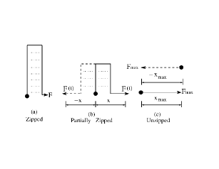
Figure 1: Schematic representations of DNA: (a) zipped, (b) partially zipped, and (c) unzipped state. One end is kept fixed (indicated by the solid circle), while the other end may move in positive (shown by the solid line) or negative direction (shown by the dashed line) depending on the force direction.

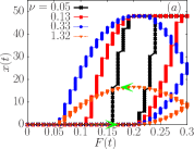
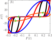
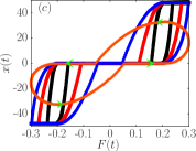
Figure 2: (Color online) Comparative plots of the area of hysteresis loop for (a) staircase and (b), (c) sinusoidal force for $F=0.33$ and chain length $L=24$. In (c) the over-damped limit is taken. For the sinusoidal force, $\nu$ was taken as $\nu/2$ to compare the positive branch of the hysteresis loop with the staircase force. Here $\nu$ is given in units of $10^{-3}$.

When a DNA chain is driven by an oscillatory force, a finite relaxation time produces a lag between force and response, and hence produces hysteresis maren ; kapri ; kumar ; arxiv1 ; mishra ; kapri1 . The area of hysteresis loop, $A_{\rm loop}$, under a periodic force with amplitude $F$ and frequency $\nu$ was found numerically in a rather detailed model to scale as $F^{\alpha}\nu^{\beta}$ kumar . Here, $\alpha$ and $\beta$ are the characteristic exponents similar to the ones seen in the case of isotropic spin systems madan1 ; madan2 ; dd ; bkc . Using Langevin dynamics (LD) simulations for different chain lengths, Mishra et al. mishra found that these exponents remain independent of solvent quality (varying friction coefficient) and interactions involved in the stability of bio-molecules (e.g., native interaction for DNA and non-native interaction for a polymer globule). Moreover, they also reported the dependence of loop area on the length of the chain, which shows a power-law scaling. In the low-frequency regime, the area of the hysteresis loop per nucleotide $A_{\rm loop}/N$ scales as $F^{0.5}\nu^{0.5}N^{0.75}$, where $N$ is the total number of nucleotides. However, scaling arguments suggest that $A_{\rm loop}/N$ should scale as $N^{0.5}$. In the high-frequency limit, $A_{\rm loop}$ remains independent of the chain length with $\alpha=2$ and $\beta=-1$. Employing Monte Carlo simulations on two interacting directed random walks, Kapri kapri1 observed that in the high-frequency limit, the scaling exponents remain the same, whereas at low frequency, he reported $\alpha=1$ and $\beta=5/4$. At this stage, there is no unanimity, thus these discrepancies must be resolved either by longer simulations based on the realistic model of DNA or through a minimal model for which an analytic solution can be derived.

The model and method adopted in Ref. kumar can describe equilibrium and non-equilibrium aspects of DNA quite well Li ; rkm ; nath ; cieplak ; libio , but simulations of longer chain length appear to be computationally challenging. An analytical solution of this model is not easy because of the many degrees of freedom involved. The aim of this work is to successively reduce the complexity of the model system and to identify the distinguishing degrees of freedom and parameters involved and thereby to develop a minimal model to understand the underlying mechanism behind the robustness of these scaling exponents.

In this spirit, we first revisited the mesoscopic model proposed in Ref. kumar and performed LD simulations Allen ; Smith at different temperatures ($T=0.1,0.08,$ and $0.06$) for a fixed length ($N=32$). Remarkably, for all these temperatures, the values of the exponents remain the same. Thus, one can speculate that these exponents are insensitive to temperature and for a better understanding of the dynamics, the system can also be studied at $T=0$. In the following, we consider two interacting strings of length $L$ (Fig. 1) to model DNA text0 . One end of the DNA is fixed, and an oscillatory force $F(t)$ is applied on the other end. The total energy of such system can be expressed as

$$E=-\epsilon_{\rm bp}N_{p}+\frac{\epsilon_{\rm bp}}{2a}|x|-F(t)x\,,$$ (1)

where $N_{p}$, $\epsilon_{\rm bp}$ and $|x|$ are the total number of base pairs, the base pairing interaction and the length of the unzipped part of the DNA, respectively. The length of the completely unzipped DNA is given by $x_{\rm max}=2L=2aN_{p}$, where $a$ $(=1)$ is the distance between two adjacent bases. Following equation of motion has been used to study the dynamics of the system at $T=0$ Allen ; Smith :

$$m\frac{d^{2}{x}}{dt^{2}}=-{\zeta}\frac{d{x}}{dt}-{\epsilon}\frac{{x}}{|x|}+F(t)\,,$$ (2)

where $\epsilon\equiv\epsilon_{\rm bp}/2$ has been set equal to 0.2. Here, $m$ $(=1)$ and $\zeta$ $(=0.4)$ are the mass of the string and friction coefficient, respectively. We used the fourth-order Runge-Kutta method (RK4) to solve Eq. (2) Allen ; Smith with time step $dt=0.01$. The singularity at $x=0$ was removed by considering $x=0$ as part of one of the two non-singular domains, i.e., ${\epsilon}\frac{{x}}{|x|}$ is replaced by $\epsilon$ for $x\geq 0$ and $-\epsilon$ otherwise. This prescription leads to small oscillations of the numerical solution around $x=0$ and creates an error of the order of $dt^{4}=10^{-8}$ new . The system achieved a steady state after about 10 cycles, but we took averages after 100 cycles.

For a staircase like periodic force kumar , the force-extension ($F-x$) curves for length $L=24$ are depicted in Fig. 2(a) for different frequencies $\nu$. The qualitative nature of these curves remains the same as seen at finite temperature ($T=0.1$) in the mesoscopic model. In order to arrive at an analytic solution, we choose $F(t)=F\sin(\omega t)$, where $\omega=2\pi\nu$. In Fig. 2(b), we have plotted the $F-x$ curves for this sinusoidal force. One can see the existence of hysteresis at different frequencies, but due to the sinusoidal nature of force, the extension will also go in the negative direction text1 . In the over-damped limit, the contribution of inertia term on the l.h.s. of Eq. (2) is small and can be dropped. We perform Brownian dynamics (BD) simulations to obtain $F-x$ curves [Fig. 2(c)]. It is evident from all these plots that the qualitative behavior of the hysteresis does not change.

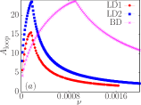
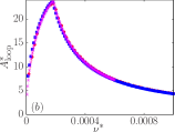
Figure 3: (Color online) (a) Variation of $A_{\rm loop}$ with $\nu$ for a staircase (LD1) and sinusoidal force (LD2) using LD simulations, and sinusoidal force using BD simulations. (b) After rescaling ($A_{\rm loop}^{*},\nu^{*}$), all three curves collapse onto a single master curve, which justifies the use of Eq. (3) for the further understanding.

For a quantitative comparison, we plot in Fig. 3(a) for all three cases the variation of $A_{\rm loop}$ with $\nu$ which exhibits a maximum that corresponds to a critical frequency dd . The variation of the loop area with frequency qualitatively remains similar to the one seen in Ref. kumar . Moreover, by rescaling the frequency $\nu^{*}=a\nu$ for the over-damped case and rescaling the area $A^{*}_{\rm loop}=bA_{\rm loop}$ for the staircase results, all three curves collapse onto a single master curve [Fig. 3(b)]. This conveys that the qualitative features and associated scaling will not change, if one performs simulations in the over-damped limit with sinusoidal force. Therefore, Eq. (2) can now be put in the following form:

$$\frac{d{x}}{dt}=\dot{x}=-\tilde{\epsilon}\frac{{x}}{|x|}+\tilde{F}\sin(\omega t),$$ (3)

where $\tilde{\epsilon}=\epsilon/\zeta$ and $\tilde{F}=F/\zeta$ are re-scaled values of $\epsilon$ and $F$, respectively. The area of the hysteresis loop scales as

$$A_{\rm loop} \simeq(\tilde{F}-\tilde{\epsilon})^{\alpha}\omega^{\beta}L^{\gamma} \simeq\left(\frac{F-F_{c}}{\zeta}\right)^{\alpha}\omega^{\beta}L^{\gamma}\,,$$ (4)

where $F_{c}\equiv\epsilon$ is the critical force for the unzipping and $\gamma$ is the exponent associated with length. Equation (4) implies that the scaling is independent of $\zeta$ text2 .

Even under this simplified description, because of the singularity at $x=0$, the analytical solution of Eq. (3) is not easy. However, imposing physical boundary conditions (discussed below), its solution has the form

$$x(t)=\begin{cases}c_{1}-\tilde{\epsilon}t-\frac{\tilde{F}}{\omega}\cos(\omega t),&\text{if }x>0\\ c_{2}+\tilde{\epsilon}t-\frac{\tilde{F}}{\omega}\cos(\omega t),&\text{if }x<0\end{cases}$$ (5)

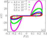
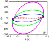
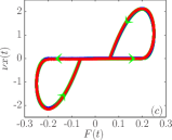
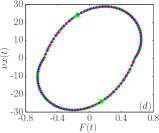
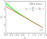
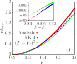
Figure 4: (Color online) (a), (b) show the $F-x$ curves at different frequencies obtained from Eq. (3) for $F=0.25$ (low) and $0.65$ (high) amplitudes, respectively. (c), (d) show the collapse of the data in (a), (b) onto a single hysteresis curve. (e) Comparison of numerical (RK4) values of $t_{2}$ as a function of $t_{1}$ with the approximate value for $\omega=1$. (f) shows the comparison of $\nu A_{\rm loop}-F$ curves obtained from different approaches [Eqs. (3), (4), and (6)]. The inset of Fig. 4(f) is a log-log plot showing that the numerical data (RK4) agree with the expansion of Eq. (6) in the limit $y\to 1$ $(F\to F_{c})$, i.e., Eq. (4) scales with $\alpha=2.5$ instead of $2$.

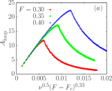
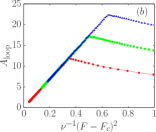
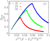
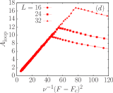
Figure 5: (Color online) Scaling of $A_{\rm loop}$ with respect to (a) $\nu^{0.5}(F-F_{c})^{0.33}$ in the low-frequency regime and (b) $\nu^{-1}(F-F_{c})^{2}$ in the high-frequency regime for a fixed length $L=24$. (c) Scaling of $\frac{A_{\rm loop}}{2L}$ with respect to $\nu^{0.5}(F-F_{c})^{0.33}L^{0.5}$ in the low-frequency regime. Each color represents here three different values of $L$. (d) Scaling of $A_{\rm loop}$ with respect to $\nu^{-1}(F-F_{c})^{2}$ for a particular value of $F$ $(=0.3)$, demonstrating the length independence in the high-frequency limit.

which (due to relaxing the constraint $|x|\leq x_{\rm max}=2L$) corresponds to the asymptotic limit $L\to\infty$. Here, $c_{1}$ and $c_{2}$ are the constants of integration, which can be evaluated by substituting $x(t)=0$. Let us assume that at time $t=0$, the DNA is in the fully zipped state. As time $t$ elapses, the magnitude of the applied force increases. If the magnitude of the applied force is less than the equilibrium critical force $F_{c}$, DNA remains in the zipped state and as a consequence the velocity of the bead, where the force is applied, remains zero. After a certain time, $t_{1}=\frac{1}{\omega}\sin^{-1}(\tilde{\epsilon}/\tilde{F})$, the applied force exceeds $F_{c}$, and the bead follows the force. After time $t^{\prime}=\frac{\pi}{2\omega}$, the magnitude of the applied force acquires its maximum value. Thus time needed to reach maximum velocity from zero is $\frac{\pi}{2\omega}-t_{1}$. With further increase in time, the extension increases until $\dot{x}$ becomes zero, i.e., up to time $t^{{}^{\prime\prime}}=\frac{\pi}{\omega}-t_{1}$. After that the extension approaches towards zero with maximum velocity. If we assume the time needed ($\frac{\pi}{2\omega}-t_{1}$) to increase the velocity from zero to maximum remains the same then the time $t_{2}$ needed to reach $x(t)=0$ can be approximated as $\frac{3\pi}{2\omega}-2t_{1}$. In Fig. 4(e) we have plotted $t_{2}$ as a function of $t_{1}$ obtained numerically [from Eqs. (3) or (5)] and from the approximate form. A nice agreement can be noticed at low force for the hysteretic state. However, these values differ at high force, where DNA always remains in the open state over the cycle. In such case, the values of $t_{1}$ and $t_{2}$ shift continuously over cycles until they acquire steady-state values after many cycles, and therefore, one has to resort to their numerical values.

The lag between the applied force and the extension constitutes hysteresis, which is depicted in Figs. 4(a) and 4(b) for low ($F=0.25$) and high ($F=0.65$) amplitudes of the force at different frequencies, respectively. In contrast to a finite chain length $L$, where the area of the hysteresis loop first increases and then decreases (Fig. 2), here, the area of the loop always increases with decreasing frequency. Multiplying numerator and denominator of Eq. (3) by $\omega$, it can be shown that $\nu x(t)$ will be a constant implying that all curves of different $\nu$ should collapse onto a single curve. This indeed we see in Fig. 4(c), (d). In fact, for a given length $L$, there exists a critical frequency $\nu_{c}$ such that for $\nu>\nu_{c}$, the scaling is $L$ independent and the system inhibits the same solution as in the limit $L\rightarrow\infty$ and vice versa.

The area of hysteresis loop $A_{\rm loop}$ may be calculated numerically. By symmetry, $A_{\rm loop}$ will be equal to $2\int_{t_{1}}^{t_{2}}F(t)\dot{x}(t)dt$. Because of the transcendental nature of Eq. (5), an analytical expression for $t_{2}$ appears to be difficult. The approximate value of $t_{2}$ discussed above [Fig. 4(e)] leads to

$$\footnotesize A_{\rm loop}=\frac{F^{2}}{\omega\zeta^{2}}\left(y(2y-3)(1+2y)\sqrt{1-y^{2}}+3\cos^{-1}(y)\right),$$ (6)

where $y=\epsilon/F$. Because of the approximation involved in $t_{2}$, Eq. (6) is still in an approximate form. In Fig. 4(f), we plot $A_{\rm loop}$ as obtained from Eqs. (3), (4), and (6) with $\nu$ for low and high amplitudes of the applied force. The nice agreement among the scaling proposed, numerical solution and analytical (approximate) solution reconfirms that the system has only one scaling. In the high-force limit, one can see from Fig. 4(f) and Eq. (6) that $A_{\rm loop}\approx\nu^{-1}F^{2}$, which is consistent with the earlier studies kumar ; mishra ; kapri1 . However, in the low-force limit ($y\to 1$), the leading term of the expansion of Eq. (6) is $\frac{42}{5}\sqrt{2}(\frac{F-F_{c}}{F_{c}})^{2.5}$, which is consistent with the numerical results [inset of Fig. 4(f)] obtained here new .

Let us now turn to the case of finite length $L$ and analyze the scaling in the low-frequency regime. For this Eq. (3) can be solved numerically by fixing $x=x_{\rm max}=2L$, over which the chain cannot be stretched. In Fig. 5(a), we show the variation of $A_{\rm loop}$ with $\nu^{0.5}(F-F_{c})^{0.33}$ in the low-frequency regime, and in Fig. 5(b) with $\nu^{-1}(F-F_{c})^{2}$ in the high-frequency limit. Interestingly, the scaling involved in frequency for low- and high-frequency regimes (Fig. 5) remains here the same compared to the model having enough mesoscopic details. The scaling associated with $F$ here is found to be equal to 0.33 and 2 in the low- and high-frequency regimes, respectively text3 . Collapse of $A_{\rm loop}/2L$ onto a single line for all lengths in the low-frequency regime confirms that the area scales with length as $L^{0.5}$ [Fig. 5(c)]. It is also evident from Fig. 5(d) that at high frequency, scaling remains independent of $L$ as predicted by Eq. (6) and seen in simulations mishra .

This paper reports many unexplored aspects of the dynamical transition associated with DNA unzipping under an oscillatory force. By successive elimination of the degrees of freedom and parameters, we developed a minimal model which presumably remains a good description for a wide range of parameters and captures the essential physics of the dynamical transition. These results are in agreement with Refs. kapri and kumar in the high-frequency limit, but strongly differ from Ref. kapri in the low-frequency regime. The analytical solution based on the minimal model provides unequivocal support for the absence of the dynamical transition in the thermodynamic limit. Moreover, scaling remains independent of temperature. The most notable outcome of the present study is the existence of a new scaling exponent associated with force in the low-force regime, which has been overlooked in all the previous studies kumar ; mishra ; kapri . While the model developed here neglects mesoscopic details, such as, excluded volume effect, spring nature of covalent bonds, helical nature of DNA, heterogeneity in the sequence etc., the robustness of the exponents suggests that it is not restricted to the study of DNA only, but may be extended to many other periodically driven complex systems cata ; exper .

We thank D. Dhar, Y. Singh, and P. Schierz for many helpful discussions on the subject. The financial assistance from the DST, New Delhi, India, the DFG Sonderforschungsbereich/Transregio SFB/TRR 102 Polymers under Multiple Constraints: Restricted and Controlled Molecular Order and Mobility, Halle-Leipzig, and the Graduate School under Grant No. CDFA-02-07 of the Deutsch-Französische Hochschule (DFH-UFA), Germany, are gratefully acknowledged.

References

- (1) B. Alberts, D. Bray, J. Lewis, M. Raff, K. Roberts, and J. D. Watson, Molecular Biology of the Cell (Garland Publishing, New York, 1994).
- (2) D. Tomkiewicz, N. Nouwen, and A. Driessen, FEBS Lett. 581, 2820 (2007).
- (3) I. Donmez and S. S. Patel, Nucleic Acids Res. 34, 4216 (2006).
- (4) M. E. Fairman-Williams and E. Jankowsky, J. Mol. Biol. 415, 819 (2012).
- (5) S. S. Velankar, P. Soultanas, M. S. Dillingham, H. S. Subramanya, and D. B. Wigley, Cell 97, 75 (1999).
- (6) D. S. Johnson, L. Bai, B. Y. Smith, S. S. Patel, and M. D. Wang, Cell 129, 1299 (2007).
- (7) A. Basu, A. J. Schoeffler, J. M. Berger, and Z. Bryant, Nat. Struct. Biol. 19, 538 (2012).
- (8) N. Fili, G. I. Mashanov, C. P. Toseland, C. Batters, M. Wallace, J. T. P. Yeeles, M. S. Dillingham, M. R. Webb, and J. E. Molloy, Nucleic Acids Res. 38, 4448 (2010).
- (9) P. Szymczak and H. Janovjak, J. Mol. Biol. 390, 443 (2009).
- (10) J. Liphardt, S. Dumont, S. B. Smith, I. Tinoco, Jr., and C. Bustamante, Science 296, 1832 (2002).
- (11) D. Collin, F. Ritort, C. Jarzynski, S. B. Smith, I. Tinoco, Jr., and C. Bustamante, Nature 437, 231 (2005).
- (12) M. Schlierf, F. Berkemeier, and M. Rief, Biophys. J. 93, 3989 (2007).
- (13) S. Kumar and M. S. Li, Phys. Rep. 486, 1 (2010).
- (14) A. K. Chattopadhyay and D. Marenduzzo, Phys. Rev. Lett. 98, 088101 (2007).
- (15) R. Kapri, Phys. Rev. E 86, 041906 (2012).
- (16) S. Kumar and G. Mishra, Phys. Rev. Lett. 110, 258102 (2013).
- (17) G. Mishra, P. Sadhukhan, S. M. Bhattacharjee, and S. Kumar, Phys. Rev. E 87, 022718 (2013).
- (18) R. K. Mishra, G. Mishra, D. Giri, and S. Kumar, J. Chem. Phys. 138, 244905 (2013).
- (19) R. Kapri, Phys. Rev. E 90, 062719 (2014).
- (20) M. Rao and R. Pandit, Phys. Rev. B 43, 3373 (1991).
- (21) M. Rao, H. R. Krishnamurthy, and R. Pandit, Phys. Rev. B 42, 856 (1990).
- (22) D. Dhar and P. Thomas, J. Phys. A 25, 4967 (1992).
- (23) B. K. Chakrabarti and M. Acharyya, Rev. Mod. Phys. 71, 847 (1999).
- (24) G. Mishra, D. Giri, M. S. Li, and S. Kumar, J. Chem. Phys. 135, 035102 (2011).
- (25) R. K. Mishra, G. Mishra, M. S. Li, and S. Kumar, Phys. Rev. E 84, 032903 (2011)
- (26) S. Nath, T. Modi, R. K. Mishra, D. Giri, B. P. Mandal, and S. Kumar J. Chem. Phys. 139, 165101 (2013).
- (27) M. S. Li and M. Cieplak, Phys. Rev. E 59, 970 (1999).
- (28) M. S. Li, Biophys. J. 93, 2644 (2007).
- (29) M. P. Allen and D. J. Tildesley, Computer Simulations of Liquids (Oxford University Press, New York, 1987).
- (30) D. Frenkel and B. Smit, Understanding Molecular Simulation (Academic Press, London, 2002).
- (31) R. Kumar, S. Kumar, and W. Janke, to be published.
- (32) The energy of the model system in Ref. kumar involves a Lennard-Jones potential, which is computationally expensive.
- (33) To avoid this, one can use . The area of the loop will then remain the same, but the frequency will be half compared to the staircase.
- (34) This has also been seen in simulations, however, an analytical argument was beyond the scope of the model in Ref. kumar .
- (35) We revisited the model discussed in Ref. kumar and analyzed the scaling in the low-frequency limit. We found that the loop area in this case also scales as , whereas the authors of Ref. kumar have used to fit their data.
- (36) D. Kumar, S. Ghosh, and S. Bhattacharya, Phys. Rev. E 87, 013202 (2013).
- (37) R. Berkovich, R. I. Hermans, I. Popa, G. Stirnemann, S. Garcia-Manyes, B. J. Berne, and J. M. Fernandez, PNAS 109, 14416 (2012).