An energy-consistent model of dislocation dynamics in an elastic body

Abstract

We propose an energy-consistent mathematical model for motion of dislocation curves in elastic materials using the idea of phase field model. This reveals a hidden gradient flow structure in the dislocation dynamics. The model is derived as a gradient flow for the sum of a regularized Allen-Cahn type energy in the slip plane and an elastic energy in the elastic body. The obtained model becomes a 3D-2D bulk-surface system and naturally includes the Peach-Koehler force term and the notion of dislocation core. We also derive a 2D-1D bulk-surface system for a straight screw dislocation and give some numerical examples for it.

1 Introduction

A dislocation or a dislocation curve is a crystallographic line defect within a crystal structure which was first studied by E. Orowan, M. Polanyi and G.I. Taylor independently in 1934. It is considered as a main mechanism of plastic deformation or yielding of the material and various material properties are studied in relation to the dislocation dynamics nowadays. See Bulatov06 ; Nabarro67 and references therein for more details.

Some properties of dislocations are as follows. In many cases, a dislocation is a plane curve in a fixed slip plane, and is the boundary of a region shifted by the Burgers vector $b\in\mathbb{R}^{3}\setminus\{0\}$. The Burgers vector is tangential to the slip plane and coincides with a translation vector of the crystal structure. Although end points often appear on the material surface or at other defects inside in a real crystal material, it is known from a topological argument that a dislocation curve cannot have an end point inside of the crystal lattice. Its typical length is around $10^{-6}$ m, typical thickness is around $10^{-9}$ m, and typical velocity is $10^{-6}$–$10^{2}$ m/s.

A dislocation generates a stress field around it by deforming the crystal structure, and interacts with other dislocations, defects, and far field conditions through the stress field. The virtual force from the stress field acting on the dislocation is called the Peach-Koehler force Bulatov06 .

There are some mathematical models of dislocations (see Bulatov06 and references therein), however, the following mathematical difficulties exist. The displacement $u$ has a jump along the dislocation curve and it has infinite elastic energy ($u\not\in H^{1}_{\mathrm{loc}}$). Therefore the elasticity equation is valid only outside of the dislocation core of radius about $5|b|$, where $|b|$ corresponds to the interatomic spacing.

In this paper, we construct an energy-consistent model in a mathematically clear way by means of the idea of the phase field Carter97 . We suppose a quasi-stationary condition, which means that the small deformation and the stress field of the material are described by the static linear elasticity equations. In other words, they are given by a minimum energy state of a suitable elastic energy. Our phase field model for the dynamics of a dislocation will be derived as a gradient flow of a total energy including the elastic one, as an analogy to the Allen-Cahn equation Chen92 ; Fife88 .

We denote a dislocation curve by $\Gamma(t)$. In this paper, we assume the dislocation curve $\Gamma(t)$ is a smooth Jordan curve in a plane. The plane which includes the dislocation curve is called the slip plane. The crystal lattice has a defect along the dislocation curve and the defect is represented by the Burgers vector $b\in\mathbb{R}^{3}\setminus\{0\}$. We suppose that $b$ is tangential to the slip plane. Let $\tau\in\mathbb{R}^{3}$ be a counterclockwise tangential unit vector of the dislocation curve $\Gamma(t)$ and let $n\in\mathbb{R}^{3}$ be one of the two possible directions of the unit normal vector of $\Gamma(t)$ tangential to the slip plane. We call the directions $n$ and $-n$ “outward” and “inward”, respectively, in this paper. We choose a unit normal vector $\nu\in\mathbb{R}^{3}$ of the slip plane with which $(n,\tau,\nu)$ is a right-handed orthonormal coordinate system. See Fig. 1 and Fig. 2 for a typical configuration.

One of the simplest mathematical models for the motion of a dislocation curve is Minarik10

$$V=-c\kappa+f,\qquad\text{on}\quad\Gamma(t),$$ (1)

where $V$ is the outward normal velocity of $\Gamma(t)$ in the slip plane and $\kappa$ is the inward signed curvature of the dislocation when considered as a plane curve. The equation (1) is called the mean curvature flow and is a typical mathematical model of phase transition. It is also known that it appears as a singular limit problem of the Allen-Cahn equation Chen92 ; Fife88 .

The term $f$ in (1) represents a far-field interaction through an elastic field from other dislocation curves including $\Gamma(t)$ itself, other defects, and boundary conditions. It is known that there is a virtual force $F\in\mathbb{R}^{3}$ acting on the dislocation curve which is given by the Peach-Koehler formula Bulatov06

$$F=\tau\times(\sigma b),$$ (2)

where $\sigma\in\mathbb{R}^{3\times 3}_{{\mathrm{sym}}}$ is the stress tensor field, $b\in\mathbb{R}^{3}$ is the Burgers vector, and $\tau\in\mathbb{R}^{3}$ is the unit tangential vector of $\Gamma(t)$. Then the term $f$ in (1) is formally given by the $n$-direction component of the Peach-Koehler force $F$. Hence, we obtain

$$f=F\cdot n=(\tau\times(\sigma b))\cdot n=(n\times\tau)\cdot(\sigma b)=\nu\cdot(\sigma b)=(\sigma\nu)\cdot b.$$ (3)

The Peach-Koehler formula, however, has the following mathematical problem. If we treat the dislocation as a one-dimensional curve $\Gamma(t)$, then the stress field $\sigma$ mathematically has a singularity along the dislocation curve as we see in Sect. 2.1 and there is no pointwise value of $\sigma$ on $\Gamma(t)$. Furthermore, the stress field must have infinite energy under a most naive setting of the problem if the dislocation curve is a mathematically sharp one-dimensional object. These mathematical singularities seem to be physically regularized due to the existence of a minimum scale given by the size of atoms and lattice spacing. In physics, this problem is often solved by introducing the notion of dislocation core which is a tubular region around the dislocation line of thickness of about $5|b|$ (see Bulatov06 ).

In this paper, we consider a regularized mathematical model of the motion of dislocation curves by means of phase field modeling. The model is derived as a gradient flow of an energy in a mathematically systematic way, and we show that it naturally includes the Peach-Koehler force in Sect. 2. A simplified 2D-1D model is also derived in Sect. 3 and its numerical examples are presented in Sect. 4.

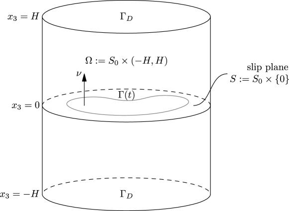
Figure 1: A typical configuration of an elastic body with a closed dislocation curve in a slip plane.

[width=0.4]figs/fig-2

Figure 2: A slip plane with a dislocation curve $\Gamma(t)$. The phase field $\varphi$ approximately satisfies $\varphi\approx 1$ in $D(t)$ and $\varphi\approx 0$ in $S\setminus D(t)$.

2 An energy-based approach to modeling of dislocation dynamics

In this section, we study displacement field in an elastic body with a dislocation, and observe that the total elastic energy is infinite without any regularization. A phase field model is proposed by introducing a regularized energy in Sect. 2.3.

2.1 Elastic energy with dislocation

We start from a homogeneous elastic body without dislocation. We denote it by $\Omega$ which is a bounded Lipschitz domain in $\mathbb{R}^{3}$. The position vector in $\bar{\Omega}$ is denoted by $x=(x_{1},x_{2},x_{3})^{{\mathrm{T}}}\in\bar{\Omega}\subset\mathbb{R}^{3}$, where ^T denotes the transpose of a vector or matrix. All vectors are assumed to be column vectors in this paper. We use the following notation: $\partial_{j}:=\frac{\partial}{\partial x_{j}}$, $\nabla=(\partial_{1},\partial_{2},\partial_{3})^{{\mathrm{T}}}$, $\nabla^{{\mathrm{T}}}u=(\partial_{j}u_{i})\in\mathbb{R}^{3\times 3}$ and $\nabla u^{{\mathrm{T}}}=(\nabla^{{\mathrm{T}}}u)^{{\mathrm{T}}}$ for $u(x)\in\mathbb{R}^{3}$. We often use Einstein’s summation convention for the space variables. For matrices $A=(a_{ij})$, $B=(b_{ij})\in\mathbb{R}^{3\times 3}$, their inner product is denoted by $A:B:=a_{ij}b_{ij}$.

Small deformation of the elastic body is described by a displacement field $u(x)=\big{(}u_{1}(x),u_{2}(x),u_{3}(x)\big{)}^{{\mathrm{T}}}\in\mathbb{R}^{3}$, the symmetric strain tensor $e[u](x)=(e_{ij}[u](x))$:

$$e[u]:=\frac{1}{2}\big{(}\nabla^{{\mathrm{T}}}u+\nabla u^{{\mathrm{T}}}\big{)}\in\mathbb{R}^{3\times 3}_{{\mathrm{sym}}},\quad\text{i.e.},\quad e_{ij}[u]=\frac{1}{2}\big{(}\partial_{j}u_{i}+\partial_{i}u_{j}\big{)},$$ (4)

and the stress tensor $\sigma[u](x)=\big{(}\sigma_{ij}(x)\big{)}\in\mathbb{R}^{3\times 3}_{{\mathrm{sym}}}$:

$$\sigma[u](x)=C(x)e[u](x),\quad\text{i.e.,}\quad\sigma_{ij}(x)=c_{ijkl}(x)e_{kl}(x),$$

where $C(x)=\big{(}c_{ijkl}(x)\big{)}\in\mathbb{R}^{3\times 3\times 3\times 3}$ is the (anisotropic) elasticity tensor with the symmetries $c_{ijkl}=c_{klij}=c_{jikl}$, $i,j,k,l\in\{1,~{}2,~{}3\}$. It should satisfy the positivity condition:

$$^{\exists}c_{*}>0\quad\text{s.t.}\quad c_{ijkl}(x)\xi_{ij}\xi_{kl}\geq c_{*}|\xi|^{2},\qquad^{\forall}x\in\Omega_{0},\ ^{\forall}\xi\in\mathbb{R}^{3\times 3}_{{\mathrm{sym}}},$$ (5)

where $|\xi|:=\sqrt{\xi_{ij}\,\xi_{ij}}$. It depends on the elastic property of the material $\Omega$ and is supposed to be given. If the material is homogeneous, the elasticity tensor should be constant $C(x)\equiv C$. From the strain-displacement relation (4), we write $\sigma[u]:=C\,e[u]$.

The displacement field $u(x)$ is obtained by the following linear second order elliptic boundary value problem:

$$\left\{\begin{aligned} -\partial_{j}\sigma_{ij}[u]&=f_{i}(x),&i=1,2,3,\ x&\in\Omega,\\ u&=g(x),&x&\in\Gamma_{{\mathrm{D}}},\\ \sigma[u]\nu&=f^{{\mathrm{N}}}(x),&x&\in\Gamma_{{\mathrm{N}}}.\end{aligned}\right.$$ (6)

where $f(x)=\big{(}f_{1}(x),f_{2}(x),f_{3}(x)\big{)}^{{\mathrm{T}}}\in\mathbb{R}^{3}$ is a given body force, and the first equation represents the equilibrium equations of force. The boundary $\partial\Omega$ is divided into two parts as

$$\partial\Omega=\Gamma_{{\mathrm{D}}}\cup\Gamma_{{\mathrm{N}}},\qquad\Gamma_{{\mathrm{D}}}\cap\Gamma_{{\mathrm{N}}}=\emptyset,\qquad|\Gamma_{{\mathrm{D}}}|>0,$$

where $\Gamma_{{\mathrm{D}}}$ is an open non-empty portion of $\Gamma$. The two dimensional area of $\Gamma_{D}$ is denoted by $|\Gamma_{{\mathrm{D}}}|$. On the other hand, $\Gamma_{{\mathrm{N}}}$ can be empty. The outward unit normal vector to $\partial\Omega$ at $x\in\partial\Omega$ is denoted by $\nu(x)\in\mathbb{R}^{3}$. The displacement on $\Gamma_{{\mathrm{D}}}$ is given by $g\in H^{\frac{1}{2}}(\Gamma_{{\mathrm{D}}};\mathbb{R}^{3})$, and the surface outer force on $\Gamma_{{\mathrm{N}}}$ is given by $f^{{\mathrm{N}}}\in L^{2}(\Gamma_{{\mathrm{D}}};\mathbb{R}^{3})$, as prescribed boundary values.

Under suitable regularity conditions, it is well-known that a unique solution to the problem (6) is given by the unique minimizer of a total elastic energy

$$E_{1}(u):=\int_{\Omega}\left\{w[u]-f\cdot u\right\}\mathop{}\!\mathrm{d}x-\int_{\Gamma_{{\mathrm{N}}}}f^{{\mathrm{N}}}\cdot u\mathop{}\!\mathrm{d}s,$$ (7)

with the boundary condition $u=g$ on $\Gamma_{{\mathrm{D}}}$, where $w[u]$ is the strain energy density defined as $w[u]:=\frac{1}{2}\sigma[u]:e[u]$.

In case that the elastic material is isotropic and homogeneous, the elasticity tensor has the form

$$c_{ijkl}=\lambda\delta_{ij}\delta_{kl}+\mu(\delta_{ik}\delta_{jl}+\delta_{il}\delta_{jk}),$$

where $\lambda\geq 0$ and $\mu>0$ are called the Lamé constants. Since

$$c_{ijkl}\xi_{ij}\xi_{kl}=\lambda(\mathrm{tr}\,\xi)^{2}+2\mu|\xi|^{2},\qquad\xi\in\mathbb{R}^{3\times 3}_{{\mathrm{sym}}},$$

the condition (5) is satisfied with $c_{*}=2\mu$. The stress tensor and the strain energy density become

$$\sigma[u]=\lambda(\operatorname{div}u)I+2\mu e[u],\qquad w[u]=\frac{1}{2}\lambda(\operatorname{div}u)^{2}+\mu|e[u]|^{2},$$

where $I$ denotes the unit tensor. The equilibrium equations of force are often called the Navier or Navier-Cauchy equations and take the following form:

$$-\mu\Delta u-(\lambda+\mu)\nabla(\operatorname{div}u)=f,\qquad\text{in }\Omega.$$ (8)

Let us now consider the case that $\Omega$ contains a dislocation curve $\Gamma(t)$. We assume that $\Gamma(t)$ is a closed plane curve without self-intersections in a fixed crystallographic plane $\tilde{S}\subset\mathbb{R}^{3}$ and define $S:=\tilde{S}\cap\Omega$, which is called the slip plane. We suppose that $S$ is connected and open in $\tilde{S}$. The Burgers vector of $\Gamma(t)$ is denoted by $b\in\mathbb{R}^{3}\setminus\{\bm{0}\}$ which is a fixed vector tangential to $S$. This is a so-called mixed dislocation which contains both edge and screw dislocations at the parts of $\Gamma(t)$ where $b\perp\Gamma(t)$ and $b\parallel\Gamma(t)$, respectively.

Choosing a suitable orthogonal coordinate system, without loss of generality, we suppose that $\tilde{S}=\{x=(x_{1},x_{2},x_{3})^{{\mathrm{T}}};\ x_{3}=0\}$, $b=(b_{1},0,0)^{{\mathrm{T}}}$, and $b_{1}>0$. A typical example of $\Omega$ and $S$ is shown in Fig. 1 and Fig. 2, where

$$\Omega=S_{0}\times(-H,H),\qquad\Gamma_{{\mathrm{D}}}=S_{0}\times\{-H,H\},\qquad\Gamma_{{\mathrm{N}}}=\partial S_{0}\times[-H,H].$$

We often identify the slip plane $S=S_{0}\times\{0\}$ with $S_{0}\subset\mathbb{R}^{2}$, if no confusion occurs. The coordinate in $S\cong S_{0}\subset\mathbb{R}^{2}$ is denoted by $x^{\prime}=(x_{1},x_{2})^{{\mathrm{T}}}$. We consider $\Gamma(t)$ and $S$ as subsets of $\mathbb{R}^{2}$, and a two dimensional domain enclosed by $\Gamma(t)$ in $S$ is denoted by $D(t)\subset S\subset\mathbb{R}^{2}$.

We define $\Omega^{\pm}:=\{(x_{1},x_{2},x_{3})^{{\mathrm{T}}}\in\Omega;\ \pm x_{3}>0\}$ and denote the outward unit normal vectors on $\partial\Omega^{\pm}$ by $\nu^{\pm}$, respectively. It is considered that the displacement field $u$ is discontinuous across the slip plane $S$. The traces of $u$ to $S$ from $\Omega^{+}$ and $\Omega^{-}$ are denoted by $u^{+}$ and $u^{-}$, respectively, and normal tractions $\sigma[u]\nu$ from $\Omega^{+}$ and $\Omega^{-}$ on $S$ are denoted by $\sigma^{+}\nu$ and $\sigma^{-}\nu$, respectively, where we define $\nu=(0,0,1)^{{\mathrm{T}}}$ on $S$. We also denote the outward unit normal vector on $\partial\Omega$ by $\nu$. We remark that $\nu=\nu^{\pm}$ on $\partial\Omega\cap\partial\Omega^{\pm}$ and that $\nu=\mp\nu^{\pm}$ on $S$. The gaps of the displacement and the traction across the slip plane $S$ are denoted by $\langle u\rangle_{S}:=u^{+}-u^{-}$ and $\langle\sigma\rangle_{S}\nu:=\sigma^{+}\nu-\sigma^{-}\nu$, respectively.

For a fixed time $t$, it is naturally expected that the displacement field $u(x)$ in $\Omega$ satisfies the following boundary value problem in a naive setting:

$$\left\{\begin{aligned} -\partial_{i}\sigma_{ij}[u]&=f_{j}(x),\quad j=1,2,3,&x&\in\Omega^{+}\cup\Omega^{-},\\ u&=g(x),&x&\in\Gamma_{{\mathrm{D}}},\\ \sigma[u]\nu&=f^{{\mathrm{N}}}(x),&x&\in\Gamma_{{\mathrm{N}}},\\ \langle u\rangle_{S}&=\begin{cases}b,&\quad\text{on}\ D(t),\\ 0,&\quad\text{on}\ S\setminus D(t),\end{cases}\\ \langle\sigma[u]\rangle_{S}\nu&=0,\qquad\text{on}\ S.\end{aligned}\right.$$ (9)

This problem, however, has no finite energy solution as seen below. Let us suppose that $u$ is a finite energy solution, i.e., $u|_{\Omega^{\pm}}\in H^{1}(\Omega^{\pm};\mathbb{R}^{3})$. Then its traces $u^{\pm}$ and $\langle u\rangle_{S}$ should belong to $H^{1/2}(S;\mathbb{R}^{3})$ but it contradicts the fourth condition of (9). In the next section, we consider a weak formulation of a jump problem in general form and study the condition that its solution has a finite energy.

2.2 Weak formulations for jump problems

We study a weak formulation for a linear elasticity problem with a jump condition across an interface like (9) in a general setting.

Under the same condition of (9), for a $\mathbb{R}^{3}$-valued function $\Psi$ on $S$, we consider the following problem

$$\left\{\begin{aligned} -\partial_{j}\sigma_{ij}[u]&=f_{i}(x),\quad i=1,2,3,&x&\in\Omega^{+}\cup\Omega^{-},\\ u&=g(x),&x&\in\Gamma_{{\mathrm{D}}},\\ \sigma[u]\nu&=f^{{\mathrm{N}}}(x),&x&\in\Gamma_{{\mathrm{N}}},\\ \langle u\rangle_{S}&=\Psi,&&\text{on }S,\\ \langle\sigma[u]\rangle_{S}\nu&=0,&&\text{on }S.\end{aligned}\right.$$ (10)

We suppose that $\Psi\in H^{\frac{1}{2}}(S;\mathbb{R}^{3})$ and $g\in H^{\frac{1}{2}}(\Gamma_{{\mathrm{D}}};\mathbb{R}^{3})$. For the problem (10), we define function spaces:

$$X :=\big{\{}w\in L^{2}(\Omega;\mathbb{R}^{3});\ w|_{\Omega^{\pm}}\in H^{1}(\Omega^{\pm};\mathbb{R}^{3})\big{\}},$$

$$X(\Psi) :=\big{\{}w\in X;\ \langle w\rangle_{S}=\Psi\big{\}},$$

$$V(g,\Psi) :=\big{\{}w\in X(\Psi);\ w=g\text{ on }\Gamma_{{\mathrm{D}}}\big{\}},$$

$$V :=V(0,0),$$

where $\langle w\rangle_{S}=w^{+}-w^{-}$ on $S$ for $w\in X$. The space $X$ is a Hilbert space with the following norm and a corresponding inner product:

$$\|w\|_{X}:=\left(\|w\|_{H^{1}(\Omega^{+};\mathbb{R}^{3})}^{2}+\|w\|_{H^{1}(\Omega^{-};\mathbb{R}^{3})}^{2}\right)^{\frac{1}{2}}.$$

We can identify $X(0)=H^{1}(\Omega;\mathbb{R}^{3})$. We remark that $X$ is a space of finite energy displacements with a gap across $S$. In the following lines, we suppose that $V(0,\Psi)\neq\emptyset$.

If $u|_{\Omega^{\pm}}\in H^{2}(\Omega^{\pm};\mathbb{R}^{3})$, and $u$ satisfies the equations of (10), $u$ is called a strong solution to (10), where the boundary conditions are considered in the sense of the trace operator. We also define a weak solution as follows.

Problem 2.1.

Find $u\in V(g,\Psi)$ such that

$$\int_{\Omega\setminus S}\sigma[u]:e[w]\mathop{}\!\mathrm{d}x-\int_{\Omega}f\cdot w\mathop{}\!\mathrm{d}x-\int_{\Gamma_{{\mathrm{N}}}}f^{{\mathrm{N}}}\cdot w\mathop{}\!\mathrm{d}s=0,\quad\text{for all}\quad w\in V.$$ (11)

A solution of Problem 2.1 is called a weak solution to (10). In particular, it is not difficult to show that a strong solution to (10) is a weak solution, by a standard computation with integration by parts. More precisely, we have the following theorem.

Theorem 2.2.

Suppose that $f\in L^{2}(\Omega;\mathbb{R}^{3})$, $f^{{\mathrm{N}}}\in L^{2}(\Gamma_{{\mathrm{N}}},\mathbb{R}^{3})$, $g\in H^{\frac{1}{2}}(\Gamma_{{\mathrm{D}}};\mathbb{R}^{3})$ and $\Psi\in H^{\frac{1}{2}}(S;\mathbb{R}^{3})$. Then, $u$ is a strong solution to (10) if and only if $u$ is a weak solution and $u|_{\Omega^{+}}$ and $u|_{\Omega^{-}}$ belong to $H^{2}(\Omega^{+};\mathbb{R}^{3})$ and $H^{2}(\Omega^{-};\mathbb{R}^{3})$, respectively.

The unique existence of the weak solution is guaranteed as follows.

Theorem 2.3.

Under the same conditions of Theorem 2.2, there exists a unique solution $u$ to Problem 2.1 and $u$ is given as a unique minimizer of $E_{1}(u)$ in $V(g,\Psi)$.

We omit the proofs of these theorems here and postpone them until our forthcoming paper. Here we just admit that the weak solution uniquely exists and let our argument proceed.

On the other hand, if $\Psi$ does not belong to $H^{1/2}(S;\mathbb{R}^{3})$ as in the dislocation model (9), there is no finite energy solution since $\Psi$ cannot be expressed by $\langle u\rangle_{S}$ for any $u\in X$. According to the model (9), the displacement field $u$ has to have a singularity along the dislocation curve with infinite elastic energy, and of course this is not a realistic solution. In a microscopic description of a crystal lattice, it is considered that this singularity is somehow regularized by the existence of a minimum length corresponding to the height of an atom. In the next section, we introduce a regularization in terms of phase field approach.

2.3 Regularization of energy

We consider a regularization for the curvature flow model (1) by means of an Allen-Cahn-type bistable potential energy. Let $\varphi$ be a phase field which is a smooth scalar-valued function defined on $S\times[0,T)$ and the value is approximately $1$ in $D(t)$ and $0$ in $S\setminus\overline{D(t)}$. For positive parameters $\varepsilon>0$ and $\beta>0$, we define an interface energy as

$$E_{0}(\varphi):=\int_{S}\left(\frac{\varepsilon}{2}|\nabla^{\prime}\varphi|^{2}+\beta W(\varphi)\right)\mathop{}\!\mathrm{d}x^{\prime},$$ (12)

where $W(s)=s^{2}(1-s)^{2}$. As its gradient flow in $L^{2}(S)$, we have the following Allen-Cahn equation

$$\alpha\frac{\partial\varphi}{\partial t}=\varepsilon\Delta^{\prime}\varphi-\beta W^{\prime}(\varphi),\qquad\text{in}\ S\times(0,T),$$ (13)

where $\nabla^{\prime}$ and $\Delta^{\prime}$ represent the gradient and the Laplacian with respect to $x^{\prime}=(x_{1},x_{2})^{{\mathrm{T}}}$. It is known that the interface energy (12) and the Allen-Cahn equation correspond to the length of the curve $\Gamma(t)$ and a motion by line tension, respectively, under a suitable scaling Fife88 .

Using this regularized interface energy $E_{0}(\varphi)$ together with the elastic energy $E_{1}(u)$ defined by (7), we consider the following total energy:

$$E(\varphi):=E_{0}(\varphi)+E_{1}(u_{\varphi}),\qquad\varphi\in H^{1}(S),$$

where $u_{\varphi}$ is a unique solution of (11) with $u_{\varphi}\in V(g,b\varphi)$.

Let us derive an $L^{2}$ gradient flow of the energy $E(\varphi)$. For a smooth scalar function $\psi$ defined on $S$, we consider a first variation:

$$\frac{d}{dr}E(\varphi+r\psi)|_{r=0}=\frac{d}{dr}E_{0}(\varphi+r\psi)|_{r=0}+\frac{d}{dr}E_{1}(u_{\varphi+r\psi})|_{r=0}.$$ (14)

The first term is formally given as

$$\frac{d}{dr}E_{0}(\varphi+r\psi)|_{r=0}=\int_{S}\big{(}-\varepsilon\Delta^{\prime}\varphi+\beta W^{\prime}(\varphi)\big{)}\psi\mathop{}\!\mathrm{d}x^{\prime}+\int_{\partial S}\frac{\partial\varphi}{\partial\nu^{\prime}}\psi\mathop{}\!\mathrm{d}s^{\prime},$$

where $\nu^{\prime}\in\mathbb{R}^{2}$ denotes the outward unit normal vector on $\partial S\cong\partial S_{0}$. For the second term of (14), it is easy to show that $u_{\varphi+r\psi}=u_{\varphi}+ru_{*}\in V(g,b(\varphi+r\psi))$ where $u_{*}$ is a unique solution of the following weak form:

$$u_{*}\in V(0,b\psi),\qquad\int_{\Omega\setminus S}\sigma[u_{*}]:e[w]\mathop{}\!\mathrm{d}x=0,\quad\text{for all}\quad w\in V.$$ (15)

Then, under suitable regularity conditions, we obtain

$$\frac{d}{dr}E_{1}(u_{\varphi+r\psi})|_{r=0} =\frac{d}{dr}E_{1}(u_{\varphi}+ru_{*})|_{r=0}$$

$$=\int_{\Omega^{+}\cup\Omega^{-}}\big{\{}\sigma[u_{\varphi}]:e[u_{*}]-f\cdot u_{*}\big{\}}\mathop{}\!\mathrm{d}x-\int_{\Gamma_{{\mathrm{N}}}}f^{{\mathrm{N}}}\cdot u_{*}\mathop{}\!\mathrm{d}s$$

$$=\int_{\partial\Omega^{+}}(\sigma[u_{\varphi}]\nu^{+})\cdot u_{*}\mathop{}\!\mathrm{d}s+\int_{\partial\Omega^{-}}(\sigma[u_{\varphi}]\nu^{-})\cdot u_{*}\mathop{}\!\mathrm{d}s$$

$$\qquad-\int_{\Omega^{+}\cup\Omega^{-}}\big{\{}\operatorname{div}\sigma[u_{\varphi}]+f\big{\}}\cdot u_{*}\mathop{}\!\mathrm{d}x-\int_{\Gamma_{{\mathrm{N}}}}f^{{\mathrm{N}}}\cdot u_{*}\mathop{}\!\mathrm{d}s$$

$$=\int_{S}\big{\{}(-\sigma^{+}[u_{\varphi}]\nu)\cdot u_{*}^{+}+(\sigma^{-}[u_{\varphi}]\nu)\cdot u_{*}^{-}\big{\}}\mathop{}\!\mathrm{d}x^{\prime}$$

$$\qquad+\int_{\Gamma_{{\mathrm{N}}}}(\sigma[u_{\varphi}]\nu-f^{{\mathrm{N}}})\cdot u_{*}\mathop{}\!\mathrm{d}s$$

$$=-\int_{S}(\sigma[u_{\varphi}]\nu)\cdot\langle u_{*}\rangle_{S}\mathop{}\!\mathrm{d}x^{\prime}$$

$$=-\int_{S}(\sigma[u_{\varphi}]\nu)\cdot b\psi\mathop{}\!\mathrm{d}x^{\prime}.$$

Hence, using the homogeneous Neumann boundary condition $\frac{\partial\varphi}{\partial\nu^{\prime}}=0$ on $\partial S$, we obtain

$$\frac{d}{dr}E(\varphi+r\psi)|_{r=0}=\int_{S}\big{(}-\varepsilon\Delta^{\prime}\varphi+\beta W^{\prime}(\varphi)-(\sigma[u_{\varphi}]\nu)\cdot b\big{)}\psi\mathop{}\!\mathrm{d}x^{\prime}.$$

Similarly to the Allen-Cahn equation (13), we derive a gradient flow of the energy $E(\varphi)$. Therefore, we propose the following phase field model for dislocation dynamics

$$\left\{\begin{aligned} \alpha\frac{\partial\varphi}{\partial t}&=\varepsilon\Delta^{\prime}\varphi-\beta W^{\prime}(\varphi)+(\sigma[u_{\varphi}]\nu)\cdot b,&\text{in}&\ S\times(0,T),\\ \frac{\partial\varphi}{\partial\nu^{\prime}}&=0,&\text{on}&\ \partial S\times(0,T),\\ \varphi(\cdot,0)&=\varphi_{0},&\text{on}&\ S,\end{aligned}\right.$$ (16)

where $\varphi_{0}(x^{\prime})$ is a suitable initial value for $\varphi$. The additional force term $(\sigma[u_{\varphi}]\nu)\cdot b$ appearing above is nothing but the Peach-Koehler force (3) acting on the dislocation line. The model (16) naturally contains the notion of the dislocation core and the Peach-Koehler force. The gradient flow structure

$$\frac{d}{dt}E(\varphi(\cdot,t))=-\alpha\int_{S}\left|\frac{\partial\varphi}{\partial t}(x^{\prime},t)\right|^{2}\,dx^{\prime}\leq 0,$$ (17)

behind the dynamics of dislocation curve has been revealed in the derivation of the model as above.

Remark.

In this paper, we treat only the case where the dislocation is a closed plane curve without any end point in the slip plane. On the other hand, it is often observed in real materials that two end points are fixed at some defect of the crystal structure. It is also known that the dislocation curve sometimes can change its slip plane. For example, some numerical simulations of dislocations with end points which change their slip planes are shown in Paus12 . The model presented in this paper can also be applied in the case where the end points are fixed on the boundary of the slip plane, if we impose the Dirichlet boundary condition of the phase field variable $\varphi$ as illustrated in Figure 3. However, the treatment of the change of the slip plane as shown in Paus12 in our model seems challenging but difficult at present.

Figure 3: Another possible configuration of the dislocation curve with fixed end points in our model is shown. The Dirichlet boundary condition for $\varphi$ is imposed as $\varphi|_{\Gamma_{0}}\approx 0$ and $\varphi|_{\Gamma_{1}}\approx 1$.

3 A simplified 2D-1D model

In this section, we derive a 2D-1D coupled phase field model for dynamics of a straight screw dislocation line in the same manner as the 3D-2D model of the previous section.

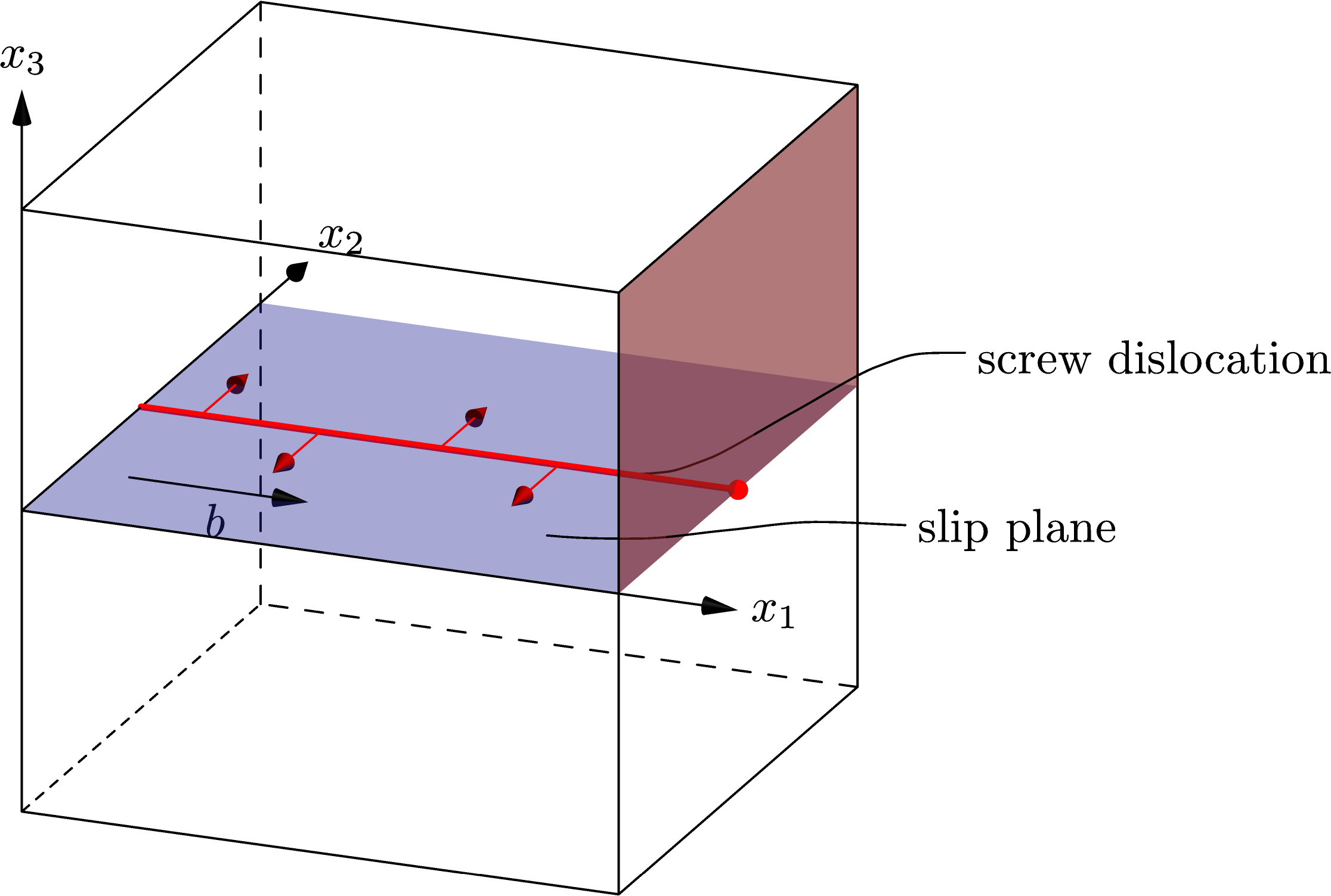
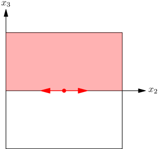
Figure 4: A straight screw dislocation in a slip plane and its two dimensional projection.

As shown in Fig. 4, we consider a rectangular parallelepiped elastic body and a slip plane in $x_{1}x_{2}$ plane. A straight screw dislocation with the Burgers vector $(b,0,0)^{{\mathrm{T}}}$ is assumed to be moving in the slip plane. In the following lines, we denote the coordinate $(x_{2},x_{3})$ also by $(x,y)$ for simplicity. For the displacement field, we suppose the so-called anti-plane displacement and an odd symmetry with respect to the slip plane $y=0$, i.e., the displacement has the form $(u(x,y),0,0)^{{\mathrm{T}}}$ and $u(x,-y)=-u(x,y)$. Then the equilibrium equation (8) becomes $-\mu\Delta u=0$, where no body force is supposed.

In the following sections, we set a rectangular two-dimensional domain $\Omega:=(-L,L)\times(0,H)$ in $xy$ plane. We define the bottom boundary $S:=(-L,L)\times\{0\}$, the lateral boundary $\Gamma_{0}:=\{-L,L\}\times[0,H]$, and top boundary $\Gamma_{1}:=(-L,L)\times\{H\}$. Then $\partial\Omega=S\cup\Gamma_{0}\cup\Gamma_{1}$ holds. The Laplacian with respect to $(x,y)$ is denoted by $\Delta=\frac{\partial^{2}}{\partial x^{2}}+\frac{\partial^{2}}{\partial y^{2}}$.

Let $u(x,y,t)\in\mathbb{R}$ be an anti-plane displacement at time $t$ and position $(x,y)\in\Omega$. Similarly to Sect. 2.3, we introduce a phase field variable $\varphi\in H^{1}(-L,L)$ and define the following total energy. We suppose that an anti-plane boundary traction $g(x)$ is given on the top boundary $\Gamma_{1}$. We set $F(s)=s^{2}(1-s)^{2}$ and define

$$E(\varphi) :=E_{0}(\varphi)+E_{1}(u_{\varphi}),$$

$$E_{0}(\varphi) :=\int_{-L}^{L}\left(\frac{\varepsilon}{2}|\varphi_{x}|^{2}+\beta F(\varphi)\right)\mathop{}\!\mathrm{d}x,$$

$$E_{1}(u) :=\mu\int\int_{\Omega}|\nabla u|^{2}\mathop{}\!\mathrm{d}x\mathop{}\!\mathrm{d}y-2\int_{\Gamma_{1}}gu\mathop{}\!\mathrm{d}x,$$

where $u_{\varphi}\in H^{1}(\Omega)$ is given as the unique weak solution to

$$\left\{\begin{aligned} \Delta u&=0,&\text{ in }&\Omega,\\ u_{x}&=0,&\text{ on }&\Gamma_{0},\\ \mu u_{y}&=g(x),&\text{ on }&\Gamma_{1},\\ u&=\frac{b}{2}\varphi(x),&\text{ on }&S.\end{aligned}\right.$$ (18)

Let us derive an $L^{2}$-gradient flow of the energy $E(\varphi)$. Under the Neumann boundary condition $\varphi_{x}(-L)=\varphi_{x}(L)=0$, for a smooth function $\psi$ defined on $S$, we consider a first variation

$$\frac{d}{dr}E(\varphi+r\psi)|_{r=0}=\frac{d}{dr}E_{0}(\varphi+r\psi)|_{r=0}+\frac{d}{dr}E_{1}(u_{\varphi+r\psi})|_{r=0}.$$ (19)

The first term is formally given as

$$\frac{d}{dr}E_{0}(\varphi+r\psi)|_{r=0}=\int_{-L}^{L}\left(-\varepsilon\varphi_{xx}+\beta F^{\prime}(\varphi)\right)\psi\mathop{}\!\mathrm{d}x.$$

It is easy to show that $u_{\varphi+r\psi}=u_{\varphi}+\frac{1}{2}rbw\in V(g,\varphi+r\psi)$, where $w\in H^{1}(\Omega)$ is the unique weak solution of

$$\left\{\begin{aligned} \Delta u&=0,&\text{ in }&\Omega,\\ u_{x}&=0,&\text{ on }&\Gamma_{0},\\ u_{y}&=0,&\text{ on }&\Gamma_{1},\\ u&=\psi(x),&\text{ on }&S.\end{aligned}\right.$$

Then the second term of (19) becomes

$$\frac{d}{dr}E_{1}(u_{\varphi+r\psi})|_{r=0} =\frac{d}{dr}E_{1}(u_{\varphi}+\frac{1}{2}rbw)|_{r=0}$$

$$=\mu b\iint_{\Omega}\nabla u_{\varphi}\cdot\nabla w\mathop{}\!\mathrm{d}x\mathop{}\!\mathrm{d}y-b\int_{\Gamma_{1}}gw\mathop{}\!\mathrm{d}x$$

$$=\mu b\int_{\partial\Omega}\frac{\partial u_{\varphi}}{\partial\nu}w\mathop{}\!\mathrm{d}s-\mu b\iint_{\Omega}(\Delta u_{\varphi})w\mathop{}\!\mathrm{d}x\mathop{}\!\mathrm{d}y-b\int_{\Gamma_{1}}gw\mathop{}\!\mathrm{d}x$$

$$=-\mu b\int_{S}\frac{\partial u_{\varphi}}{\partial y}\psi\mathop{}\!\mathrm{d}x.$$

Hence, we obtain

$$\frac{d}{dr}E(\varphi+s\psi)|_{r=0}=\int_{-L}^{L}\left(-\varepsilon\varphi_{xx}+\beta F^{\prime}(\varphi)-\mu b\frac{\partial u_{\varphi}}{\partial y}(x,0)\right)\psi\mathop{}\!\mathrm{d}x.$$

Similarly to the Allen-Cahn equation (13), we derive a gradient flow of the energy $E(\varphi)$ as

$$\alpha\varphi_{t}=\varepsilon\varphi_{xx}-\beta F^{\prime}(\varphi)+b\mu\frac{\partial u_{\varphi}}{\partial y}(x,0),\qquad x\in(-L,L),\ t>0.$$ (20)

The additional force term $b\mu\frac{\partial u_{\varphi}}{\partial y}(x,0)$ is formally corresponding to the Peach-Koehler force (3) acting on the screw dislocation. We substitute the relation

$$\varphi(x,t)=\frac{2}{b}u_{\varphi}(x,0,t),\qquad x\in[-L,L],~{}t\geq 0,$$

into (20) and set

$$W(s):=\frac{4\beta}{b^{2}}s^{2}\left(\frac{b}{2}-s\right)^{2},\qquad\gamma:=\frac{\mu b^{2}}{2}.$$

The boundary load $g(x)$ is also assumed to depend on time $t$. Then, we obtain the following 2D-1D dislocation model:

$$\left\{\begin{aligned} \Delta u&=0,&(x,y)&\in\Omega,\ t\in[0,T],\\ u_{x}&=0,&(x,y)&\in\Gamma_{0},\ t\in[0,T],\\ u_{y}&=g(x,t),&(x,y)&\in\Gamma_{1},\ t\in[0,T],\\ \alpha u_{t}&=\varepsilon u_{xx}-W^{\prime}(u)+\gamma u_{y},&(x,y)&\in S,\ t\in(0,T],\\ u&=u_{0}(x),&(x,y)&\in S,\ t=0.\end{aligned}\right.$$ (21)

4 Numerical results

In this section, we give some numerical examples for an approximation of (21).

We discretize (21) by employing standard finite differences to approximate spatial derivatives. A rectilinear grid is obtained by dividing $\Omega$ into $N_{x}\times N_{y}$ rectangular cells and a solution is sought at the grid nodes. This spatial discretization results in a non-linear system of ODEs in time that we solve by means of a fully implicit, variable-step solver CVode .

The initial condition in both examples below is a shifted and scaled Heaviside function $u_{0}(x)=bH(x-x_{0})$ where $x_{0}$ is the initial position of the step. Other parameter values used in the numerical examples are summarized in Table 1.

In both figures below the horizontal axis corresponds to the spatial $x$ variable while the vertical axis corresponds to the time. We plot the graph of $u$ at $S$ at 50 time levels distributed uniformly in $[0,T]$, the initial condition $u_{0}$ being the lowest graph with the time increasing upwards. The graph of $u$ in the whole of $\Omega$ is not shown.

$T$	$L$	$H$	$N_{x}$	$N_{y}$	$b$	$\varepsilon$	$\beta$	$\mu$	$\alpha$
4	2	2	256	128	0.06	0.04	10	10	0.01

Table 1: Parameter values used in numerical examples for the model (21).

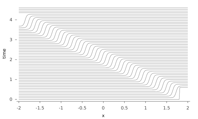
Figure 5: Numerical example of a screw dislocation moving under a constant loading.

In Fig. 5 we present a numerical example of a screw dislocation that moves in a stress field caused by a constant anti-plane traction imposed on the top boundary $\Gamma_{1}$. We set $g\equiv 0.5$ and place the dislocation at the initial location $x_{0}=1.8$. The dislocation moves to the left at an almost constant velocity until it reaches the crystal surface at $x=-2$ where it annihilates.

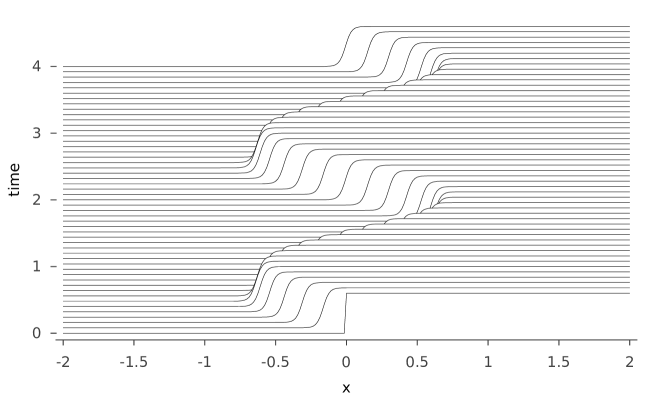
Figure 6: Numerical example of a screw dislocation moving under a periodic loading.

In Fig. 6 we consider the behaviour of a screw dislocation under a periodic loading. We place the dislocation at $x_{0}=0$ and set $g(x,t)=\cos(0.5t)$. The oscillating stress field causes the dislocation to move periodically around its initial location.

5 Summary and Conclusions

We proposed a 3D-2D phase field model (16) for dynamics of a mixed dislocation curve and a 2D-1D model (21) for a straight screw dislocation. They are both derived as gradient flows of regularized total energies and naturally include the Peach-Koehler force and the notion of the dislocation core. Some numerical examples of the 2D-1D model are given in Sect. 4. The revealed gradient flow structure (17) is expected to be useful for further mathematical and numerical analysis.

One of interesting questions about this model is the relation between the layer width of $\varphi$ (i.e., the radius of the dislocation core) and the parameters $\varepsilon$, $\beta$ and $|b|$. This is still open but seems to be important not only in the sense of modeling but also in numerical simulations for choosing a proper mesh size.

References

- (1) Alvarez, O., Carlini, E., Hoch, P., Le Bouar, Y., Monneau, R.: Dislocation dynamics described by non-local Hamilton-Jacobi equations. Materials Science and Engineering A 400–401, 162–165 (2005); doi: 10.1016/j.msea.2005.01.062
- (2) Bulatov, V., Cai, W.: Computer Simulations of Dislocations. Oxford Series on Materials Modelling, Oxford University Press (2006)
- (3) Carter, W.C., Taylor, J.E., Cahn, J.W.: Variational methods for microstructural evolutions. JOM 49, 30–26 (1997); doi: 10.1007/s11837-997-0027-2
- (4) Chen, X.: Generation and propagation of interfaces for reaction-diffusion equations. Journal of Differential Equations 96, 116–141 (1992); doi: 10.1016/0022-0396(92)90146-E
- (5) Cohen, S.D., Hindmarsh, A.C.: CVODE, A Stiff/Nonstiff ODE Solver in C. Computers in Physics 10(2), 138–143 (1996)
- (6) Fife, P.C.: Dynamics of Internal Layers and Diffusive Interfaces. CBMS-NSF Regional Conference Series in Applied Mathematics 53, SIAM, Philadelphia, PA, (1988); doi: 10.1137/1.9781611970180
- (7) Hirsch, P.B., Horne, R.W., Whelan, M.J.: Direct observations of the arrangement and motion of dislocations in aluminium. Philosophical Magazine 1, 677–684 (1956); doi: 10.1080/14786435608244003
- (8) Minárik, V., Beneš, M., Kratochvíl, J.: Simulation of dynamical interaction between dislocations and dipolar loops. Journal of Applied Physics 107, 061802 (2010); doi: 10.1063/1.3340518
- (9) Nabarro, F.R.N.: Theory of Crystal Dislocations. Clarendon Press, Oxford (1967)
- (10) Pauš, P., Beneš, M., Kratochvíl, J.: Simulation of dislocation annihilation by cross-slip. Acta Physica Polonica A, 122, No.3, 509–5011 (2012)