Mechanical Yield in Amorphous Solids: a First-Order Phase Transition

Abstract

Amorphous solids yield at a critical value of the strain (in strain controlled experiments); for larger strains the average stress can no longer increase - the system displays an elasto-plastic steady state. A long standing riddle in the materials community is what is the difference between the microscopic states of the material before and after yield. Explanations in the literature are material specific, but the universality of the phenomenon begs a universal answer. We argue here that there is no fundamental difference in the states of matter before and after yield, but the yield is a bona-fide first order phase transition between a highly restricted set of possible configurations residing in a small region of phase space to a vastly rich set of configurations which include many marginally stable ones. To show this we employ an order parameter of universal applicability, independent of the microscopic interactions, that is successful in quantifying the transition in an unambiguous manner.

A ubiquitous, and in fact universal, characteristic of the mechanical properties of amorphous solids is their stress vs. strain dependence 98Ale . Measured in countless quasi-static strain-controlled simulations (see for example 04VBB ; 04ML ; 05DA ; 06TLB ; 06ML ; 09LP ; 11RTV ) and experiments (see for example 06SLG ; 13KTG ; 13NSSMM ), it typically exhibits two distinct regions. In one region, at lower strain values, the stress ${\bm{\sigma}}$ increases on the average upon the increase of strain ${\bm{\gamma}}$, although this increase is punctuated by plastic events. A second region, at higher values of the strain, displays a constant (on the average) stress which cannot increase even though the strain keeps increasing. Of course also this elasto-plastic steady state branch is punctuated by plastic events. A typical such shear stress vs. shear strain curve at zero temperature is shown in Fig. 1. The two regions are separated by what is referred to as “yield”. The actual shape of the stress vs. strain curve near the yield point depends on details of the system preparation. Amorphous solids prepared by a slow quench from the melt tend to display a stress peak before yielding, whereas those prepared by a fast quench join the steady state smoothly without a stress peak 13JBP . Of course the steady state branch itself is independent of the preparation protocol; memory of the initial state is lost in this regime.

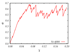
Figure 1: A typical stress vs. strain curve obtained in a strain-controlled athermal quasistatic (AQS) shearing protocol using a Kob-Andersen 65-35% Lennard Jones Binary Mixture of 4000 particles in $2d$. Note the generic existence of a pre-yield branch in which the stress is increasing on the average when the strain increases, and a post yield steady state where the average stress is constant. Both regions are punctuated by plastic events, with the stress drops being much larger in the post-yield compared to the pre-yield branch. This kind of stress vs. strain curve is ubiquitous for a huge variety of amorphous solids. Here and in the text we drop tensorial indices from the stress and the strain for notational simplicity.

The phenomenon of the mechanical yield in amorphous solids has been a subject of extensive study in recent years. Many numerical studies on the subject have been performed using athermal, quasi-static shear (AQS) protocols, wherein a glass is made by quenching a glass former down to zero temperature, and then subjecting it to a quasi-static ($\dot{\gamma}\to 0$) shear protocol wherein the system is subject to small shear steps, and then allowed, after each step, to find a new mechanically stable minimum of its potential energy. This kind of protocol always gives rise to the same basic kind of phenomenology as seen in Fig. 1 independently of the detailed microscopic interaction between the constituents. This basic phenomenology has been reported in very many publications, and there is a general consensus about the fact that a qualitative change of some sort must take place between the “elastic” and “steady-state” parts of the stress-strain curve. As much as the qualitative picture is evident, however, a lot of difficulty arises when trying to capture this qualitative change in a quantitative manner.

Devising a way to distinguish and study two different states of matter, and the transition that connects one with the other, means identifying an order parameter to act as a label for the states. This, however is a challenging program in the present case: as much as the “elastic” and “steady state” branches look different (one is able to increase the stress under a shear load, while the other cannot), a snapshot, say, of a particle configurations in both regimes is unable to detect any relevant difference between the two. Since both states are anyway amorphous, there is no trivial order parameter that would allow us to unambiguously tell them apart. Notice how this difficulty is not present in the case of crystalline solids, which do exhibit evident structural peculiarities with respect to liquids, and whose mechanism of failure is well known since decades. Ultimately, it all boils down to finding a suitable order parameter for the glass phase.

The problem of finding an order parameter for a glass is both practical and conceptual. First, as we said before, a snapshot of a typical glass configuration before and after yield does not show any difference: all glasses look the same to us, and all of them look like a liquid. Standard methods like structure functions, higher order correlation functions, Voronoi tesselations, Delaunay triangulations etc. all failed to provide distinction between typical configurations before and after yield.

In this Letter we propose that the difficulty in making a distinction between the pre- and post-yield configurations lies in the fact that there is really no distinction. The crux of the matter is not in the nature of configurations but in their number. The yield takes place because of a sudden opening up of a vast number of configurations that are not at the system’s disposal before yield. To establish this insight we employ an order parameter of a type that was found useful first in the context of spin glasses 97FP . Following Refs. 97FP ; 10CCGGGPV ; 12YM ; 13Ber ; 14BC ; 14BCTT ; 15BJ ; 15NBC we can define an order parameter with the idea of comparing two different glassy configurations $\{{\bm{r}}^{(1)}_{i}\}_{i=1}^{N}$ and $\{{\bm{r}}^{(2)}_{i}\}_{i=1}^{N}$ ,

$$Q_{12}\equiv\frac{1}{N}\sum_{i}^{N}\theta(a-|{\bm{r}}^{(1)}_{i}-{\bm{r}}^{(2)}_{i}|)\ ,$$ (1)

wherein $\theta(x)$ is the Heaviside step function. The value of the parameter $a$ is free, and is determined by trial and error. The quantity $Q_{12}$ is called an “overlap” since it has a value that goes from $0$ (completely decorrelated configurations) to $1$ (perfect correlation). Its purpose is to measure the degree of similarity between configurations.

Let us now consider a glass, made by quenching a super-cooled liquid with $N$ particles down to a certain temperature $T\geq 0$ at a suitable rate. A glass is an amorphous solid wherein particles vibrate around an amorphous structure. So, if we take two configurations $\{{\bm{r}}_{i}^{(1)}\}_{i=1}^{N}$ and $\{{\bm{r}}_{i}^{(2)}\}_{i=1}^{N}$ from this glass, they will be most likely close to each other with $Q_{12}$ of the order of unity. If one is able to obtain a good sampling of the typical configurations visited by the particles in the glass, one can measure the probability distribution of the overlap $P(Q_{12})$, which will be strongly peaked around an average value $\langle Q_{12}\rangle$ close to unity. The configurations visited by the particles will then form a small connected “patch” in the configuration space of the system, selected by the amorphous structure provided by the last configuration that was visited by the liquid glass former before it fell out of equilibrium while forming a glass.

Imagine now that we begin to strain this glass. While the stress increases, there exist plastic events that begin to cause irreversible displacements in the particle positions. Our order parameter $Q_{12}$ will begin to respond to these displacements and will begin to reduce from $O(1)$ to lower values. We will show now that all along the “elastic” branch $\langle Q_{12}\rangle$ will remain around unity, but as the mechanical yield takes place a sharp phase transition occurs, whereupon sub-extensive plastic events 09LP2 ; 12DHP ; 13DGMPZ begin to cause substantial displacements, allowing different regions of the configuration space to affect the order parameter. In such a situation, the distribution $P(Q_{12})$ will have two peaks: one at high $Q_{12}\leq 1$ corresponding to configurations in the same patch and one for $Q_{12}\geq 0$ corresponding to configurations in different patches.

To demonstrate this fundamental idea we can use any model glass, since this order parameter description is expected to be universal. For concreteness we performed molecular dynamics simulations of a Kob-Andersen 65-35% Lennard Jones Binary Mixture in $2d$. We have two system sizes, $N=500$ and $N=4000$. We chose $Q_{12}$ with $a=0.3$ in LJ units, but verified that changes in $a$ leave the emerging picture invariant. As a first step, we prepared a glass by equilibrating the system at $T=0.4$, and then quenching it (the rate is $10^{-6}$) down to $T=1\cdot 10^{-6}$ into a glassy configuration. The sample is then heated up again to $T=0.2$, and a starting configuration of particle positions is chosen at this temperature. Note that while at $T=0.4$ equilibration is sufficiently fast, at $T=0.2$ the computation time is much shorter than the relaxation time. The configuration is then assigned a set of velocities randomly drawn from the Maxwell distribution at $T=0.2$, and these different samples are then quenched down to $T=0$ at a rate of $0.1$. This procedure can be repeated any number of times (say 500 times), and it allows us to get a sampling of the configurations inside one single “patch”. We verify that the typical overlap of the ensemble of inherent structures so obtained in one patch is close to $\langle Q_{12}\rangle=1$, signaling that indeed the ensemble is completely located in a single patch. Having one patch, we repeat the procedure starting from another equilibrated configuration of the liquid to create another patch. The results shown below for the system with 4000 particles were obtained by having 100 different patches, each of which containing 500 different inherent structures due to the velocity randomization. The results with 500 particles were based on 520 different patches each of which having 100 different inherent structures.

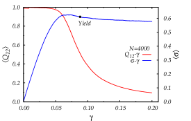
Figure 2: a superposition of a stress vs strain curve on the dependence of $\langle Q_{12}\rangle$ on $\gamma$. The stress vs. strain curve is obtained by averaging over 50,000 realizations of individual such curves obtained from 100 initial patches, each of which containing 500 inherent structures. The order parameter $Q_{12}$ was averaged on the same realizations to provide $\langle Q_{12}\rangle$.

We then apply to each inherent structure an AQS protocol as described above. This will create for each value of $\gamma$ a strained ensemble of configurations in the patch whose $P_{\gamma}(Q_{12})$ is measured. The order parameter is computed by using all the unique pairs of configuration generated in the strained ensemble at a given $\gamma$. We present the results for $N=4000$ in Fig. 2. We can see how the initial ensemble for $\gamma=0$ shows a value of the order parameter $Q_{12}=1$, signifying that our initial ensemble is genuinely within one patch. As the ensemble is strained, the value of the order parameter gets lower, dropping towards zero when the strain is increased beyond the yield strain.

To determine the yield strain $\gamma_{{}_{Y}}$ accurately, we consider the probability distribution function (pdf) $P_{\gamma}(Q_{12})$. We determine $P_{\gamma}(Q_{12})$ for each patch of of 500 configurations obtained as explained above, and then average the result over the 100 available patches. We ask at which value of $\gamma$ this averaged pdf has two equally high peaks, see Fig 3. The resulting $\langle P_{\gamma}(Q_{12})\rangle$ determines the yield point to occur at $\gamma_{{}_{Y}}\simeq 0.088$. Note that this criterion implies a sharp definition of “yield” which seems absent in the current literature. If accepted, it indicates that the mechanical yield occurs beyond the stress overshoot in correspondence with the mean-field results of Ref. 15RUYZ .

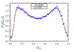
Figure 3: The probability distribution function $P_{\gamma}(Q_{12})$ at $\gamma_{{}_{Y}}=0.088$ averaged over 100 initial configurations each of which has 500 different realizations to obtain $\langle P_{\gamma}(Q_{12})\rangle$. At this value of the strain the pdf has two peaks of equal heights. We identify this value of $\gamma$ as the point of the phase transition.

Once we identify the phase transition point, we can demonstrate the transition itself. In Fig. 4 we display the change in $\langle P_{\gamma}(Q_{12})\rangle$ in the vicinity of the critical point $\gamma_{{}_{Y}}$ as a function of $\gamma$.

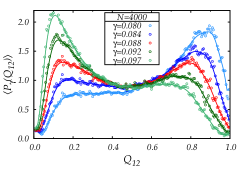
Figure 4: The probability distribution function $\langle P_{\gamma}(Q_{12})\rangle$ in the vicinity of the critical point $\gamma_{{}_{Y}}=0.088$

Within a very narrow range of $\gamma$, of the order of $\Delta\gamma\approx 0.017$, we observe a first-order like transition from a pdf with dominant peak at high values of $Q_{12}$ to a dominant peak at low values of $Q_{12}$. We capture a very unambiguous and qualitative change in behavior as the yielding point is reached.

To sharpen the understanding of what is happening in the vicinity of the yield point we examine next how many of our realizations loose the tight overlap with the initially prepared configuration and where the loss of overlap is taking place. To this aim we consider, for the system of 4000 particles, all the 50,000 realizations that we have. These are obtained by 100 choices of liquid realizations, each of which is velocity randomized 500 times (chosen with Boltzmann probabilities). When the strain $\gamma$ is increased in our AQS algorithm, we keep computing the order parameter $Q_{12}$ where the first configuration $\{{\bm{r}}^{(1)}_{i}\}_{i=1}^{N}$ in Eq. (1) is chosen randomly from all the available configurations at that value of $\gamma$, and the second is any one of the other available configurations at the same value of $\gamma$. We confirmed that changing the randomly chosen $\{{\bm{r}}^{(1)}_{i}\}_{i=1}^{N}$ does not affect the results. Next, choosing $Q_{12}=0.8$ as a threshold value, we now count how many of our observed configurations cross this threshold and exhibit $Q_{12}\leq 0.8$. The number of configurations that do so as a function of the strain (superimposed on the stress.vs. strain curve) is shown in Fig 5.

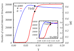
Figure 5: The number of configurations which pass below the threshold value $Q_{12}=0.8$ of the overlap order parameter as a function of the strain $\gamma$ for $N=4000$. In the onset we show the same test for $N=500$. The conclusion is that all the configurations lose overlap with the initial configuration in the vicinity of the yield point $\gamma_{{}_{Y}}$

.

The conclusion of this test is that in the vicinity of the yield point $\gamma_{{}_{Y}}$ all the configurations lose their overlap with the initial configuration, but not before. The mechanical yield is tantamount to the opening up of a vast number of possible configurations, whereas before yield the system is still constrained to reside in the initial meta-basin of the free energy landscape. This appears to be a first-order phase transition 16RU .

To strengthen the proposition that this is a first-order phase transition we should demonstrate that the transition becomes sharper with increasing the system size. At present we cannot produce equally good data for systems of size much larger than $N=4000$, but we have produced equally extensive data for $N=500$. The results for this smaller system size are presented in Fig. 6.

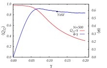
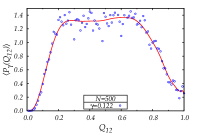
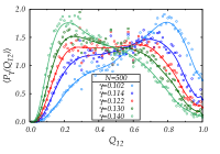
Figure 6: Results similar to those shown in Figs.2-4 but for system size $N=500$. One observes a smearing out of the transition region as is expected from a first-order phase transition.

Indeed, the change in the values of $Q_{12}$ diminishes as seen in the upper panel, the identification of the transition point is less sharp, and most importantly, the range of $\Delta\gamma$ over which a similar change in the peak structure is taking place is now $\Delta\gamma\approx 0.038$. If we take just these two system sizes as indicative we can roughly estimate the range of $\Delta\gamma$ over which the transition is taking place to go to zero as $N^{-1/3}$ as $N\to\infty$. Needless to say, at this point this should be taken as indicative only, and further accurate simulations should be conducted to solidify (excuse the pun) this important issue.

The upshot of these results is that we are able to put a finger on the essential feature that is responsible for the mechanical yield. It is not that the configurations visited by the system after yield have different characteristics from the configurations before yield. Rather, a very constrained set of configurations available to the system before yield is replaced upon yield with a vastly larger set of available configurations. This much larger set is generic; it is not selected by any careful cooling protocol, and as such it is expected to include many marginally unstable configurations that will yield plastically with any increase of strain 10KLP ; 16HJPS . This is the fundamental reason for the inability of the system to continue to increase its stress when strain is increased, leading to the steady state branch. We propose this as a universal mechanism for the ubiquitous prevalence of stress vs strain curves that look so similar in a huge variety of glassy systems.

- (1) S. Alexander, Phys. Rep. 296, 65 (1998).
- (2) F. Varnik, L. Bocquet, and J.-L. Barrat, J. Chem. Phys. 120, 2788 (2004).
- (3) C. E. Maloney and A. Lemaitre, Phys. Rev. Lett. 93, 016001 (2004).
- (4) M. J. Demkowicz and A. S. Argon, Phys. Rev. B 72, 245205 (2005).
- (5) A. Tanguy, F. Leonforte, and J.-L. Barrat, Eur. Phys. J. E 20, 355 (2006).
- (6) C. E. Maloney and A. Lemaitre, Phys. Rev. E 74, 016118 (2006).
- (7) E. Lerner and I. Procaccia, , Phys, Rev. E, 80, 026128 (2009).
- (8) D. Rodney, A. Tanguy and D. Vandembroucq, Modelling Simul. Mater. Sci. Eng. 19, (2011) 08300.
- (9) G. Subhash, Q. Liu and X-L Gao, Int. J. Impact Engineering 32 1113 (2006).
- (10) A. Kara, A. Tasdemirci and M. Guden, Materials & Design 49, 566 (2013).
- (11) A. L. Noradila, Z. Sajuri, J. Syarif, Y. Miyashita and Y. Mutoh, Materials Science and Engineering 46, 012031 (2013).
- (12) Ashwin J., E. Bouchbinder and I. Procaccia Phys. Rev. E 87, 042310 (2013).
- (13) S. Franz and G. Parisi, Phys. Rev. Lett. 79, 2486 (1997).
- (14) C. Cammarota, A. Cavagna, I. Giardina, G. Gradenigo, T. S. Grigera, G. Parisi, and P. Verrocchio, Phys. Rev. Lett. 105, 055703 (2010).
- (15) J. Yeo and M. A. Moore, Phys. Rev. E 86, 052501 (2012).
- (16) L. Berthier, Phys. Rev. E 88 , 022313 (2013).
- (17) L. Berthier and D. Coslovich, Proc. Natl. Acad. Sci. U.S.A. 111 , 11668 (2014).
- (18) G. Biroli, C. Cammarota, G. Tarjus, and M. Tarzia, Phys. Rev. Lett. 112, 175701 (2014).
- (19) L. Berthier and R.L. Jack, Phys. Rev. Lett. 114, 205701 (2015).
- (20) A. Ninarello, L. Berthier and D. Coslovich, Molecular Physics, 113, 2707 (2015).
- (21) E. Lerner and I. Procaccia, Phys. Rev. E 29, 066109 (2009).
- (22) R. Dasgupta, H. G. E. Hentschel and I. Procaccia, Phys.Rev. Lett., 109, 25502 (2012).
- (23) R. Dasgupta, O. Gendelman, P. Mishra, I. Procaccia and C. A.B.Z. Shor, Phys. Rev. E., 88, 032401 (2013).
- (24) C. Rainone, P. Urbani, H. Yoshino and F. Zamponi Phys. Rev. Lett. 114, 015701 (2015).
- (25) C. Rainone and P. Urbani, arXiv:1512.00341.
- (26) S. Karmakar, E. Lerner and I.Procaccia, Phys.Rev. E, 82, 055103(R) (2010).
- (27) H.G.E. Hentschel, P. K. Jaiswal, I.Procaccia and S. Sastry, “Stochastic Approach to Plasticity and Yield in Amorphous Solids”, ArXiv: 1509.04907