Resistor-network anomalies in the heat transport of random harmonic chain

Abstract

We consider thermal transport in low-dimensional disordered harmonic networks of coupled masses. Utilizing known results regarding Anderson localization, we derive the actual dependence of the thermal conductance $G$ on the length $L$ of the sample. This is required by nanotechnology implementations because for such networks Fourier’s law ${G\propto 1/L^{\alpha}}$ with ${\alpha=1}$ is violated. In particular we consider “glassy” disorder in the coupling constants, and find an anomaly which is related by duality to the Lifshitz-tail regime in the standard Anderson model.

I Introduction

The theory of phononic heat conduction in disordered low-dimensional networks is a central theme of research in recent years LLP03 ; D08 ; LRWZHL12 . The interest in this theme is not only purely academic, but it is also motivated by the ongoing developments in nanotechnology. In spite of the recent research efforts, the understanding of thermal transport is still at its infancy. This becomes more obvious if one compares with the achievements that have been experienced during the last fifty years in understanding and managing electron transport. In this respect even the microscopic laws that govern heat conduction in low dimensional systems have only recently start being scrutinized via both theoretical, numerical and experimental studies LLP03 ; D08 ; COGMZ08 ; NGPB09 ; LRWZHL12 ; ZL10 ; K1 ; K2 . These studies unveil many surprising results, the most dramatic of which is the violation of the naive expectation (Fourier’s law) which states that the thermal conductance $G$ is inverse proportional to the size $L$ of the system, namely, $G\propto 1/L^{\alpha}$ with ${\alpha=1}$.

Currently it is well established that in low-dimensional disordered systems, in the absence of non-linearity, Fourier’s law is violated. The underlying physics is related to the theory of Anderson localization of the vibrational modes D08 ; D01 ; LXXZL12 ; DL08 ; LD05 ; RD08 ; LZH01 ; KCRDLS10a ; KCRDLS10b . On the basis of the prevailing theory D08 ; D01 it has been claimed that for samples with “optimal” contacts ${\alpha=1/2}$, while in general $\alpha$ might be larger, say ${\alpha=3/2}$ for samples with “fixed boundary conditions”. Recently the “optimal” value ${\alpha=1/2}$ has been challenged by the numerical study of BZFK13 . These authors found a super-optimal value ${\alpha\sim 1/4}$ for moderate system sizes $L$, while asymptotically, in the presence of a pinning potential, $G$ decays exponentially as ${\exp(-\gamma L)}$.

It is obvious that if the final goal is to achieve the control of heat flow on the nanoscale, first we have to understand the fundamental mechanisms of heat conduction, and provide an adequate description of its scaling with the system size for any $L$, including the experimentally relevant cases of intermediate lengths.

II Scope

Considering heat transport for low-dimensional disordered networks of coupled harmonic masses, we utilize known results from the field of mesoscopic electronic physics, in order to derive the actual $L$ dependence of $G$ for regular as well as for “glassy” type of disorder. The information about the latter is encoded in the dependence of the inverse localization length $\gamma$ on the vibration frequency $\omega$. Our results explain the transition from optimal to super-optimal scaling behavior and eventually to exponential dependence on $L$. We address the implications of the percolation threshold, and the geometrical bandwidth. Along the way we highlight a surprising anomaly that is related by duality to the Lifshitz-tail regime in the standard Anderson model, and test the borders of the one-parameter scaling hypothesis.

The outline of this paper is as follows: Sections III-V define the general model of interest, emphasizing that for “glassy disorder” a resistor-network perspective is essential. Section VI clarifies that the analysis of heat conduction of quasi one dimensional networks effectively reduces to the analysis of a single-channel problem. Section VII explains how we use the transfer matrix method in the numerical analysis: we highlight the procedure for the determination of the optimal leads, and the significance of the percolation parameter $s$ in this context. Section VIII use the Born approximation in order to provide an explanation for the numerical findings of BZFK13 . These results had been obtained for weak disorder.

Subsequently we focus on the single-channel model. Our main interest is to explore the implications of “glassy” disorder, and to highlight the resistor-network aspect. In Sections IX and X we go beyond the born approximation by establishing a duality between glassy off-diagonal disorder and weak diagonal disorder. Consequently we deduce that the Lifshitz-tail anomaly is reflected in the frequency dependence of the inverse localization length. This prediction is verified numerically.

The remaining sections XI to XIII clarify how scaling-theory of localization can be used in order to calculate the heat conductance. Here no further surprises are found. In fact we verify numerically that a straightforward application of the weak-disorder analytical approach is quite satisfactory. In spite of the “glassy” disorder the deviations from one-parameter scaling are not alarming.

III The model

We consider a one-dimensional network of $L$ harmonic oscillators of equal masses. The system is described by the Hamiltonian

$${\cal H}={1\over 2}P^{T}P+{1\over 2}Q^{T}\bm{W}Q$$ (1)

where $Q^{T}\equiv(q_{1},q_{2},\cdots,q_{N})$, and $P^{T}\equiv(p_{1},p_{2},\cdots,p_{N})$ are the displacement coordinates and the conjugate momenta. The real symmetric matrix $\bm{W}$ is determined by the spring constants. Its off-diagonal elements $W_{nm}{=}-w_{nm}$ originate from the coupling potential $(1/2)\sum_{m,n}w_{nm}(q_{n}-q_{m})^{2}$, while its diagonal elements contain an additional optional term that originate from a pinning potential ${(1/2)\sum_{n}v_{n}q_{n}^{2}}$ that couples the masses to the substrate. Accordingly ${W_{nn}=v_{n}+\sum_{m}w_{nm}}$. For a chain with near-neighbor transitions we use the simplified notation ${w_{n{+}1,n}\equiv w_{n}}$.

In general the interest is in quasi one-dimensional networks, for which $\bm{W}$ is a banded matrix with ${1{+}2b}$ diagonals. For ${b{=}1}$ the near-neighbor hopping implies a single-channel system. For ${b>1}$ the dispersion relation (see section VI below) has several branches, which is like having a multi-channel system. The heat conduction of such networks has been investigated numerically in BZFK13 , with puzzling findings that have not been explained theoretically. We shall see that the essential physics can be reduced to single channel ($b{=}1$) analysis. On top we would like to consider not only weakly disordered network, but also the implications of “glassy” disorder as defined below.

IV The disorder

Both the $w_{nm}$ and the $v_{n}$ are assumed to be random variables. The diagonal-disorder due to the pinning potential is formally like that of the standard Anderson model with some variance ${\sigma_{\parallel}^{2}\equiv\mbox{Var}(v)}$. The off-diagonal disorder of the couplings might be weak with some variance ${\sigma_{\perp}^{2}=\mbox{Var}(w)}$, but more generally it can reflect the glassiness of the network. By “glassy disorder” we mean that the coupling $w$ has an exponential sensitivity to physical parameters. For random barrier statistics ${w\propto\mathrm{e}^{-B}}$, where $B$ is uniformly distributed within $[0,\sigma]$, accordingly

$$P(w)\ \ \propto\ \ \frac{1}{w}\ \ \left(\mathrm{e}^{-\sigma}<\frac{w}{w_{c}}<1\right)$$ (2)

For random distance statistics ${w\propto\mathrm{e}^{-R}}$, where $R$ is implied by Poisson statistics. The probability distribution in the latter case is

$$P(w)\ \ =\ \ \frac{s}{w_{c}^{s}}w^{s-1}\ (w<w_{c})$$ (3)

where $s$ is the normalized density of the sites. Large $s$ is like regular weak disorder, while small $s$ implies glassy disorder that features log-wide distribution (couplings distributed over several orders of magnitude). The case $s=0$ with an added lower cutoff formally corresponds to “random barriers”.

V Resistor-network perspective

It is useful to notice that the problem of phononic heat conduction in the absence of a pinning potential is formally equivalent to the analysis of a rate equation, where the spring-constants are interpreted as the rates $w_{nm}$ for transitions between sites $n$ and $m$. Optionally it can be regarded as a resistor-network problem where $w_{nm}$ represent connectors. We define $w_{0}$ as the effective hopping rate between sites. We later justify that it should be formally identified with the conductivity of the corresponding resistor-network.

The detailed numerical analysis in the subsequent sections concerns the ${b=1}$ chain, for which the “serial addition” rule implies that $w_{0}$ equals the harmonic average. For the “random distance” disorder of Eq.(3) we get

$$w_{0}\ =\ \left[\left\langle\frac{1}{w}\right\rangle\right]^{-1}\ =\ \ (s{>}1)\left[\frac{s-1}{s}\right]w_{c}$$ (4)

For ${s<1}$ the network is no longer percolating, namely ${w_{0}=0}$. In the present context $w_{0}$ determines the speed of sound (see below).

For the later analysis we need also the second moment of the couplings. For $s>2$ one obtains

$$\left\langle\left(\frac{1}{w}\right)^{2}\right\rangle_{s{>}2}\ =\ \left[\frac{s}{s-2}\right]\left(\frac{1}{w_{c}}\right)^{2}$$ (5)

Hence the variance is $[s/((s{-}1)^{2}(s{-}2))]w_{c}^{-2}$. For ${s<2}$ the second moment diverges. But for a particular realization the sample-specific result is finite, and depends on the effective lower cutoff $\delta w$ of the distribution. The number ${\mathcal{N}\equiv w_{c}/\delta w}$ reflects the finite size of the sample, and we get the sample-size dependent result

$$\left\langle\left(\frac{1}{w}\right)^{2}\right\rangle_{s{<}2}\ =\ \frac{s}{2{-}s}\left[\mathcal{N}^{2{-}s}-1\right]\left(\frac{1}{w_{c}}\right)^{2}$$ (6)

As we go from ${s>2}$ to ${s<2}$ the dependence of the variance on $s$ has a crossover from power-law to exponential. We shall see later that this crossover is reflected in the localization-length of the eigenstates.

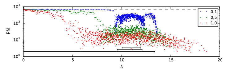
Figure 1: The participation number (PN) a of the eigenstates of a conservative banded matrix are plotted against their eigenvalues $\lambda$. The $0<|m-n|\leq b$ elements of $\bm{W}$ are random numbers $w\in[1-\varsigma,1+\varsigma]$ (box distribution). The values of $\varsigma$ are indicated in the legend (note that the numerics of BZFK13 corresponds to $\varsigma{=}0.5$). The number of bands is $b{=}5$, and the length of the sample is $N{=}1000$ with periodic boundary conditions. The support of the clean-ring channels is indicted by the lower horizontal lines. We observe the gradual blurring of the non-disordered band structure. All the eigenstates that have large PN reside in the lower part of the spectrum and belong to a single channel.

VI The spectrum

The eigenvalues $\lambda_{k}$ are determined via diagonalization $\bm{W}Q=\lambda Q$, from which one deduces the eigen-frequencies via ${\lambda_{k}=\omega_{k}^{2}}$. In the absence of disorder the eigenmodes are Bloch states with

$$\lambda_{k}\ =\ 2w_{0}\sum_{r=1}^{b}[1-\cos(rk)]\ \ \equiv\ \ \omega_{k}^{2}$$ (7)

where $k$ is the associated wavenumber. For a single-channel $\lambda=2w_{0}(1{-}\cos k)\approx w_{0}k^{2}$, where the small-$k$ approximation holds close to the band floor. With disordered couplings, but in the absence of a pinning potential the lowest eigenvalue is still ${\lambda_{0}=0}$, which corresponds to the trivial extended state ${Q=(1,1,...,1)}^{T}$, that is interpreted as the ergodic state in the context of rate equations. All higher eigenstates are exponentially localized, and are characterized by a spectral density $\varrho(\omega)$.

In Fig.1 we provide a numerical example considering a ${b=5}$ quasi-one dimensional sample. The dispersion relation Eq.(7) has 5 branches. The support of the 1st, 3rd and 5th ascending branches is indicated in the figure. It is important to observe that at the bottom of the band a single channel-approximation is most appropriate. Hence within the framework of the Debye approximation the dispersion at the bottom of the band is always

$$\omega\ \ \approx\ \ ck\ \ \ \ \ \ \ \text{[Debye]}$$ (8)

For $b{=}1$ the speed of sound is ${c=\sqrt{w_{0}}}$, while for $b{\gg 1}$ it is easily found that

$$c\ \ \approx\ \ [(1/3)b^{3}]^{1/2}\,\sqrt{w_{0}}$$ (9)

Either way the low-frequency spectral density is constant, namely

$$\rho(\omega)\ \ \approx\ \ \frac{L}{\pi c}$$ (10)

The effect of weak disorder on this result is negligible.

VII Localization

The disorder significantly affects the eigenmodes: rather than being extended as assumed by Debye, they become exponentially localized. We use the standard notation $\gamma(\omega)$ for the inverse localization length. Considering a single-channel (${b{=}1}$) system it is defined via the asymptotic dependence of the transmission $g$ on the length $L$ of the sample. Namely,

$$\gamma(\omega)\ \ =\ \ -\lim_{L\rightarrow\infty}{1\over 2}{\langle\ln(g)\rangle_{\omega}\over L}$$ (11)

where $\langle\cdots\rangle$ indicates an averaging over disorder realizations. The notion of transmission is physically appealing here, because we can regard $\bm{W}$ as the Hamiltonian of an electron in a tight binding model. The transmission can be calculated from the transfer matrix $\bm{T}$ of the sample:

$$g=\frac{4|\sin(k)|^{2}}{|T_{21}-T_{12}+T_{22}\exp(ik)-T_{11}\exp(-ik)|^{2}}$$ (12)

where

$$\bm{T}\ \ =\ \ \prod_{n=1}^{n=L}\left(\begin{matrix}\frac{\lambda-(v_{n}+w_{n}+w_{n+1})}{w_{n+1}}&-\frac{w_{n}}{w_{n+1}}\cr 1&0\end{matrix}\right)$$ (13)

Above it is assumed that the sample is attached to two non-disordered leads. Optimal coupling requires the hopping-rates there to be all equal to the “conductivity” $w_{0}$, meaning same speed of sound. This observation has been verified numerically, see Fig.2. We see that it is the resistor-network harmonic-average and not the algebraic-average that determines the optimal coupling.

In Fig.3 we display an example for the calculation of $\gamma$ versus $s$. Well-defined results are obtained for ${s>2}$ where the second moment Eq.(5) is finite. In the next section we shall derive a naive Born approximation for $\gamma$. This is displayed in Fig.3 too as a dashed line. The estimate is based on analytical ensemble-average of $\text{Var}(1/w)$ and therefore diverges as ${s=2}$ is approached from above. In the range ${1<s<2}$ the second moment Eq.(6) is ill-defined (sample-specific). Given an individual sample the Born approximation can be used with sample-variance (which is always finite) and provide a rough estimate. The typical result in this range is expected to depend exponentially on $s$ as implied by Eq.(6). This expected dependence is indeed observed. For ${s<1}$ the $s$ dependence of $\gamma$ is completely ill-defined: the chain is non-percolating in the $L\to\infty$ limit, and the contact optimization procedures becomes meaningless.

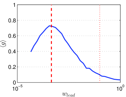
Figure 2: The average transmision $\left\langle g\right\rangle$ as a function of the hopping rate $w_{\text{lead}}$ within the leads. The calculation is done for ${L=50}$ disordered sample, where the $w_{n}$ are distributed according to Eq.(2) with ${\sigma=10}$ at ${k=0.028\pi}$. The algebraic and the harmonic mean values of the $w_{n}$ are indicated by vertical dotted and dashed lines respectively.

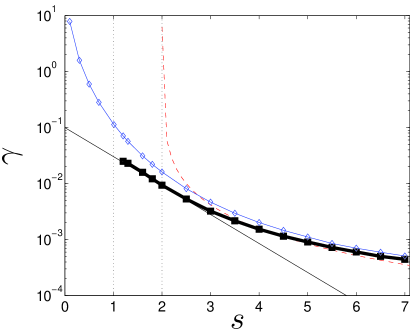
Figure 3: The inverse localization length $\gamma$ for the random distance disorder of Eq.(3) versus $s$. Solid line with diamonds is for the non-optimized (${w_{\text{lead}}=w_{c}}$) results. Thick solid line with squares is for the optimized (${w_{\text{lead}}=w_{0}}$) results in the range ${s>1}$, where $w_{0}$ is finite. The tangent thin solid line has been fitted in the range ${1<s<2}$ where Eq.(6) is expected to hold. The naive Born approximation Eq.(15) is illustrated by dashed line in the range ${s>2}$. The numerical results here and in the next figures are based on the transfer matrix method (symbols), with several hundreds of realizations up to ${L\sim 10^{4}}$.

VIII Born approximation

In the absence of disorder $\bm{W}$ describes hopping with some rate $w_{0}$, and the eigenstates are free waves labeled by $k$. With disorder the $w_{0}$ of the unperturbed Hamiltonian is loosely defined as the average $w$. Later we shall go beyond the Born approximation and will show that it should be the harmonic average (as already defined previously). The disorder couples states that have different $k$. For diagonal disorder (”pinning”) the couplings are proportional to the variance of the diagonal elements, namely ${\overline{|W_{k,k^{\prime}}|^{2}}=(1/L)\text{Var}(v)}$. For off-diagonal disorder (random spring constants) the couplings are proportional to the variance of the off-diagonal elements, and depends on $b$ and on $k$ too:

$$\overline{\left|W_{k^{\prime},k}\right|^{2}}=\frac{\text{Var}(w)}{L}\ \sum_{r=1}^{b}\left[2\sin(rk^{\prime}/2)\,2\sin(rk/2)\right]^{2}$$

It follow that for small $k$ we have ${|W_{k,k^{\prime}}|^{2}\propto b^{5}\sigma_{\perp}^{2}k^{4}}$.

The Fermi-Golden-Rule (FGR) picture implies that the scattering rate is ${\tau^{-1}=2\pi\varrho(\omega)\overline{\left|W_{k^{\prime},k}\right|^{2}}}$. The Born approximation for the mean free path is ${\ell=[d\lambda/dk]\tau}$, where the expression in the square brackets is the group velocity in the electronic sense ($\lambda$ is like energy). The Debye approximation implies $d\lambda/dk\approx 2[c^{2}]k$. The inverse localization length is $\gamma=(2\ell)^{-1}$. From here (without taking the small $k$ approximation) it follows that

$$\gamma(\omega)\ \ \approx \ \ \frac{1}{8}\left[\frac{9}{b^{6}}\right]\left(\frac{\sigma_{\parallel}}{w_{0}}\right)^{2}\left(\frac{1}{\sin(k)}\right)^{2}$$ (14)

$$+ \ \ \frac{1}{8}\left[\frac{9}{5b}\right]\left(\frac{\sigma_{\perp}}{w_{0}}\right)^{2}\left(2\tan\left(\frac{k}{2}\right)\right)^{2}$$ (15)

where the prefactors in the square brackets assume ${b\gg 1}$, and should be replaced by unity for ${b=1}$. In the absence of pinning the localization length diverges ($\gamma\propto k^{2}$) at the band floor, as assumed by Debye. This behavior is demonstrated in Fig.4 and Fig.5 for two types of glassy disorder. The deviations from Eq.(15) will be explained in the next paragraphs.

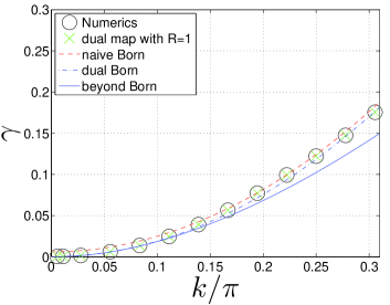
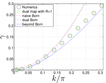
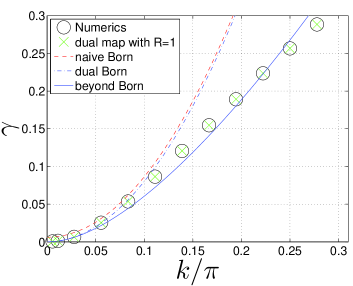
Figure 4: The inverse localization length $\gamma$ versus $k$ for the random barrier disorder of Eq.(2) with $\sigma=5,10,15$ from up to down. Pure off-diagonal disorder is assumed. The numerical results based on the transfer matrix method (circles) are compared with those that are generated by the map Eq.(20) with the approximation ${R_{n}{=}1}$. The naive Born estimate Eq.(15) is illustrated by dashed red line, while the blue dashed-dotted line is based on the improved estimate with Eq.(23). Here we consider the distribution of Eq.(2) for which both estimates coincide identically, therefore a small shift has been inserted artificially so the two lines could be discern. The inverse localization length $\gamma$ is over-estimated as $k$ becomes larger due to the Lifshitz tail anomaly. The solid blue line is based on Eq.(24) with no fitting parameters.

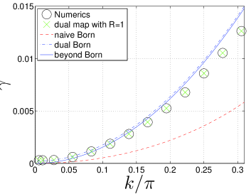
Figure 5: The inverse localization length $\gamma$ versus $k$ for the random distance disorder of Eq.(3) with $s=4$. The symbols and lines are the same as in Fig.4. Note that the “dual Born” approximation cannot be resolved from its improved version Eq.(24). Here we consider the distribution of Eq.(3) for which the duality implies $k$ dependence that does not coincide with that of the naive Born approximation.

IX Beyond Born

The Born approximation has assumed weak disorder. Here we would like to consider the more general case of glassy disorder. For this purpose, as in DG84 , we write the equation ${\bm{W}\psi=\lambda\psi}$ for the eigenstates as a map of a single variable ${r_{n}=\psi_{n}/\psi_{n-1}}$, namely ${r_{n+1}=-R_{n}/r_{n}-A_{n}}$, where ${R_{n}=w_{n-1}/w_{n}}$, and ${A_{n}=(\lambda-v_{n}-w_{n}-w_{n-1})/w_{n}}$. In the case of diagonal disorder it takes the from

$$r_{n+1}\ =\ -\frac{1}{r_{n}}-\epsilon+f_{n}$$ (16)

where $f_{n}=v_{n}/w_{0}$ is the scaled disorder and

$$\epsilon\ \ =\ \ \frac{\lambda}{w_{0}}-2\ \ \equiv\ \ -2\cos(k)$$ (17)

is the scaled energy measured from the center of the band. Without the random term $f_{n}$ this map has a fixed-point that is determined by the equation ${r^{2}+\epsilon r+1=0}$, with elliptic solution for ${\epsilon\in[-2,2]}$. The random term is responsible for having a non zero inverse localization length ${\gamma=-\langle\ln(r)\rangle}$. The Born approximation Eq.(14) is written as

$$\gamma\ \ \approx\ \ \frac{1}{8}\,\frac{\mbox{Var}(f)}{\left[1-(\epsilon/2)^{2}\right]}\ \ =\ \ \frac{1}{8}\,\frac{\mbox{Var}(f)}{[\sin(k)]^{2}}$$ (18)

This standard estimate does not hold close to the band-edge $\epsilon_{0}{=}{-}2$, which can be regarded as an anomaly DG84 . Closeness to the band-edge means that ${|\epsilon-\epsilon_{0}|}$ becomes comparable with the kinetic energy $\gamma^{2}$. Hence the so called Lifshitz tail region is ${|\epsilon-\epsilon_{0}|<\epsilon_{c}}$ with $\epsilon_{c}=[\mbox{Var}(f)]^{2/3}$. Optionally this energy scale can be deduced by dimensional analysis. In the Lifshitz tail region the inverse localization length has finite value $\gamma\sim\sqrt{\epsilon_{c}}$. An analytical expression can be derived using white-noise approximation (see Appendix A for details):

$$\gamma\ =\ \left(\frac{1}{2}\text{Var}(f)\right)^{\frac{1}{3}}\mathcal{K}\left[\Big{(}2\text{Var}(f)^{2}\Big{)}^{-\frac{1}{3}}\,k^{2}\right]\ \ \ \ \ \ \ \ \$$ (19)

Outside of the Lifshitz tail region this expression reduces back to Eq.(18). To be more precise, if we want to take the exact dispersion into account an add-hock improvement of Eq.(19) would be to to replace $k^{2}$ by $[\sin(k)]^{2}$. But our interest is in small $k$ values, for which this improvement is not required in practice: this has been confirmed numerically (not displayed).

X Duality

We now turn to consider the glassy disorder due to the dispersion of the $w_{n}$. Here we cannot trust the Born approximation because a small parameter is absent. However, without any approximation we can write the map in the form

$$r_{n+1}\ \ =\ \ R_{n}\left(1-\frac{1}{r_{n}}\right)+1-\frac{\lambda}{w_{n}}$$ (20)

For $\lambda{=}0$ the zero momentum state is a solution as expected, irrespective of the disorder: the randomness in $R_{n}$ is not effective in destroying the ${r=1}$ fixed point. Therefore, for small $\lambda$, we can set without much error ${R_{n}=1}$. The formal argument that justifies this approximation is based on the linearization ${(r_{n+1}-1)=R_{n}(r_{n}-1)}$, and the observation that the product ${R_{1}R_{2}R_{3}...}$ remains of order unity. In Fig.4 and Fig.5 we verify numerically that setting ${R_{n}{=}1}$ does not affect the determination of $\gamma$.

Having established that Eq.(20) with ${R_{n}=1}$ in a valid approximation, we realize that it reduces to Eq.(16), with zero-average random term

$$f_{n}=-\lambda\left(\frac{1}{w_{n}}-\frac{1}{w_{0}}\right)$$ (21)

This random term corresponds to the diagonal-disorder of the standard Anderson model. Consequently, the implied definition of $\epsilon$ via Eq.(17) justifies the identification of the harmonic average $w_{0}$ as the effective coupling.

We observe that there is an emergent small parameter, namely, the dispersion of $f$, which is proportional to $\lambda$ irrespective of the glassiness. Thus we have deduced a duality between “strong” glassy off-diagonal disorder and the “weak” diagonal disorder. In the context of the dual problem we can use the Born approximation Eq.(18) with

$$\mbox{Var}(f)\ \ =\ \ \left[2\sin\left(\frac{k}{2}\right)\right]^{2}w_{0}^{2}\,\mbox{Var}\left(\frac{1}{w}\right)$$ (22)

leading to Eq.(15) but with two important modifications with respect to FGR-based derivation: (i) we realize that $w_{0}$ should be the harmonic average, as conjectured in the introduction; (ii) we realize that the dispersion for off-diagonal disorder should be re-defined as follows:

$$\sigma_{\perp}^{2}\ \ :=\ \ w_{0}^{4}\ \mbox{Var}\left(\frac{1}{w}\right)$$ (23)

For log-box distribution the FGR definition $\sigma_{\perp}^{2}=\mbox{Var}(w)$ and the revised definition Eq.(23) provide exactly the same result. But for random distance disorder the two prescriptions differ enormously. This is demonstrate in Fig.4 and Fig.5, were we present our numerical results together with the theoretical predictions.

Having adopted the revised definition Eq.(23), we still see in Fig.4 and Fig.5 that the inverse localization length $\gamma$ is over-estimated as $k$ becomes larger. We can trace the origin of this discrepancy to the Lifshitz anomaly in the Anderson model. The condition ${|\epsilon-\epsilon_{0}|<\epsilon_{c}}$ translates into ${\lambda>w_{0}^{-3}[\mbox{Var}(1/w)]^{-2}}$. Thus the anomaly develops not at the band floor but as we go up in $\omega$, where the inverse localization length becomes $\gamma\propto\omega^{4/3}$ instead of $\gamma\propto\omega^{2}$. To verify that this is indeed the explanation for the deviation we base our calculation on Eq.(19), namely

$$\gamma\approx\left(\frac{1}{2}\left(\frac{\sigma_{\perp}}{w_{0}}\right)^{2}k^{4}\right)^{\frac{1}{3}}\mathcal{K}\left[\left(2\left(\frac{\sigma_{\perp}}{w_{0}}\right)^{4}k^{2}\right)^{-\frac{1}{3}}\right]\ \ \ \$$ (24)

The anomaly appears whenever the argument of $\mathcal{K}(E)$ is small, meaning large $k$ rather than small $k$. The validity of this formula is numerically established in Fig.4 and Fig.5 with no fitting parameters. We note that a slightly better version of Eq.(24) can be obtained by replacing the $k$s by appropriate trigonometric functions as implied by the remark after Eq.(19) and Eq.(22). But the numerical accuracy is barely affected by such an improvement.

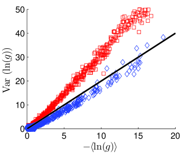
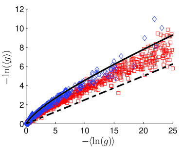
Figure 6: Testing one parameter scaling for glassy disorder. The variance of $\ln(g)$ (upper panel) and the log of the average $-\ln\langle g\rangle$ (lower panel) are plotted against the scaling parameter $-\langle\ln(g)\rangle$. The calculation is done for the random distance disorder of Eq.(3) with ${s=15}$ (blue diamonds) and ${s=1.2}$ (red squares). The solid line is the standard one parameter scaling prediction for weak disorder, and the dashed line is its asymptotic approximation. One observes that an anomaly develops as the disorder becomes glassy.

XI The average transmission

For the calculation of the heat transport we have to know what is ${g(\omega)\equiv\langle g\rangle_{\omega}}$. Given $\gamma$ the common approximation is ${\langle g\rangle\approx\mathrm{e}^{-(1/2)\gamma L}}$. But in-fact this asymptotic approximation can be trusted only for very long samples. More generally, assuming weak disorder, the following result can be derived Abrikosov ; Shapiro ; Izrailev :

$$\langle g\rangle\ =\ \int_{0}^{\infty}\mathrm{d}u\ \frac{2\pi u\tanh(\pi u)}{\cosh(\pi u)}\ \mathrm{e}^{-\left[\left(\frac{1}{4}+u^{2}\right)\gamma L\right]}$$ (25)

The question arises whether this relation can be trusted also in the case of a glassy disorder, where the one-parameter scaling assumption cannot be justified. This is tested in Fig.6. For weak disorder (large $s$) the expected relation between the first and second moments of $x=-\ln(g)$ is confirmed, namely ${\text{Var}(x)=2\langle x\rangle}$. For strong glassy disorder (small $s$) clear deviation from this relation is observed.

Still we see in Fig.6 (lower panel) that the failure of one-parameter scaling is not alarming for $\langle g\rangle=\langle\exp[-x]\rangle$. The exact calculation of the integral is the solid line, while the asymptotic result $\exp[-(1/2)\langle x\rangle]$ is indicated by dashed line. Note that the latter implies ${\langle g\rangle=\exp[(1/4)\langle\ln(g)\rangle]}$. We realize that the asymptotic approximation might be poor, but the exact calculation using Eq.(25) is quite satisfactory.

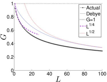
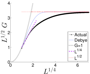
Figure 7: The heat conductance $G$ as a function of $L$ is calculated using Eq.(28) with Eq.(25). For the black solid line with symbols we use $\gamma(k)$ that is based on the numerical results that have been obtained for a random barrier disorder as in Fig.4 with ${\sigma=1}$. For the blue solid line we use the Debye approximation for the density of states, and extrapolate the initial $\gamma\propto k^{2}$ dependence up to the cutoff $k=\pi$. On the lower panel we plot $\sqrt{L}G$ as a function of $L^{1/4}$ in order to highlight the ${\alpha=1/2}$ (dotted red) and the ${\alpha=1/4}$ (dashed red) asymptotic dependence for long and short samples respectively. The black dotted line is $G=1$.

XII Heat conductance

Following D08 ; D01 ; DL08 the expression for the rate of heat flow from a lead that has temperature $T_{H}$ to a lead that has temperature $T_{C}$ is

$$\dot{Q}\ =\ \frac{T_{H}{-}T_{C}}{2}\int_{0}^{\infty}\frac{d\omega}{\pi}\ \mathcal{T}(\omega)\ \equiv\ G\,(T_{H}{-}T_{C})\ \$$ (26)

Here $\mathcal{T}(\omega)$ is a complicated expression that reflects the transmission of the sample. If we were dealing with incoherent or non-linear transport dubi , it would be possible to justify the Ohmic expression ${\mathcal{T}(\omega)=\ell/L}$, where $\ell$ is the inelastic mean free path. But we are dealing with an isolated harmonic chain, therefore ${\mathcal{T}(\omega)}$ is determined by the couplings of the eigenmodes to the heat reservoirs at the left and right leads. In analogy to mesoscopics studies D08 ; D01 one can argue that

$$\mathcal{T}(\omega)\ \ \approx\ \ g(\omega)\ \mathcal{T}^{(0)}(\omega)$$ (27)

where $\mathcal{T}^{(0)}(\omega)$ refers to a non-disordered sample, and $g(\omega)$ is the disordered averaged transmission. For “fixed boundary conditions” ${\mathcal{T}^{(0)}(\omega)\sim\eta_{0}^{2}\omega^{2}}$, where the damping rate $\eta_{0}$ characterizes the contact point. In contrast, for “free boundary condition” one obtains ${\mathcal{T}^{(0)}(\omega)\approx 1}$, which is the most optimal possibility. In the latter case

$$G\ \ =\ \ \frac{c}{2}\int_{0}^{\pi}\frac{dk}{\pi}\ g(\omega_{k})$$ (28)

The standard approach is to use two incompatible approximations: On the one hand one use the asymptotic estimate ${g(\omega)\sim\mathrm{e}^{-(1/2)\gamma(\omega)L}}$ which holds for long samples for which $\gamma L\gg 1$. On the other hand one extends the upper limit of the integration to infinity, arguing that the major contribution to the integral comes from small $\omega$ values. In the absence of pinning $\gamma(\omega)\propto\omega^{2}$, hence by rescaling of the dummy integration variable it follows that the result of the integral is precisely $\propto 1/\sqrt{L}$. We shall discuss in the next paragraph the limitations of this prediction. Going on with the same logic we can ask what happens in the presence of a weak pinning potential. Using a saddle-point estimate we get

$$G\ \ \sim\ \ \frac{1}{\sqrt{L}}\ \exp\left[-(1/2)\gamma_{0}L\right]$$ (29)

where $\gamma_{0}$ is the minimal value of $\gamma(\omega)$. From Eq.(15) with Eq.(14) we deduce $\gamma_{0}\propto b^{-\eta}$, with $\eta=7/2$. This explains the leading exponential dependence on the length that has been observed in BZFK13 . However the above calculation fails in explaining the sub-leading $L$ dependence that survives in the absence of pinning. Namely it has been observed that instead of $1/L^{\alpha}$ with $\alpha=1/2$ the numerical results are characterized by the super-optimal value ${\alpha\approx 1/4}$.

XIII Beyond the asymptotic estimate

We now focus on the $L$ dependence that survives in the absence of a pinning potential. As already note that deviation from the $1/\sqrt{L}$ law is related to two incompatible approximations regarding the $\gamma$ dependence of $g$ and the upper limit of of the integration in Eq.(28). We can of course do better by using the analytical expression Eq.(25). For the density of states we can use either numerical results or optionally we can use the Debye approximation. The latter may affect the results quantitatively but not qualitatively. Within the framework of the Debye approximation we assume idealized dependence $\gamma(\omega_{k})\propto\sigma_{\perp}^{2}k^{2}$ in accordance with Eq.(15), up to the cutoff at $k=\pi$. The result of the calculation is presented in Fig.7. On the lower panel there we plot $\sqrt{L}G$ as a function of $L^{1/4}$ in order to highlight the ${\alpha=1/2}$ and the ${\alpha=1/4}$ asymptotic dependence for long and short samples respectively. Note that in the latter case, as in BZFK13 , a small offset has been included in the fitting procedure. We do not think that the ${\alpha=1/4}$ dependence is “fundamental”. The important message here is that a straightforward application of an analytical approach can explain the failure of the $1/\sqrt{L}$ law. We also see that the numerical prefactor of the $1/L^{\alpha}$ dependence is sensitive to the line-shape of the large $k$ cutoff, hence it is not the same for the numerical spectrum and for its Debye approximation.

XIV Conclusions

We have considered in this work the problem of heat conduction of quasi one-dimensional ($b\gg 1$) as well as single channel harmonic chains; addressing the effects of both glassy disorder (couplings) and pinning (diagonal disorder). We were able to provide a theory for the asymptotic exponential length ($L$) and bandwidth ($b$) dependence; as well as for the algebraic $L$ dependence in the absence of a pinning potential. A major observation along the way was the duality between glassy disorder and weak Anderson disorder. That helped us to figure out what is the effective hopping $w_{0}$, hence establishing a relation to percolation theory. It also helped us to go beyond the naive Born approximation that cannot be justified for glassy disorder, and to identify a (dual) Lifshitz anomaly in the $\omega$ dependence of the transmission. Finally, we have established that known results from one-parameter scaling theory can be utilized in order to derive the non-asymptotic $L$ dependence of the heat conductance.

Note added after acceptance.– It has been observed in Chalker that the one-dimensional localization problem with the distribution Eq.(3) describes in a universal way the phononic excitations of a one-dimensional Bose-Einstein condensate in a random potential: the superfluid regime is percolating (${s{>}1}$), while the Mott-insulator regime corresponds to the “$s{=}0$” random-barrier distribution Eq.(2). The localization length in the anomalous regime ${1{<}s{<}2}$ had been worked out in Ziman , leading to ${\gamma\propto\omega^{s}}$, while ${\gamma\propto\omega^{2}}$ applies if ${s{>}2}$.

Acknowledgements.– We thank Boris Shapiro (Technion) for helpful comments. This research has been supported by by the Israel Science Foundation (grant No. 29/11), and by the NSF Grant No. DMR-1306984.

Appendix A Localization in white noise potential

There is an analytical expression for the counting function of the energy-levels for a particle in a white-noise disordered potential. We cite Eq(1.62) of halperin :

$$\mathcal{N}(E)\ =\ \frac{1}{\pi^{2}}\Big{(}[\text{Ai}(-2E)]^{2}+[\text{Bi}(-2E)]^{2}\Big{)}^{-1}\ \ \ \ \$$ (30)

In this expression the levels are counted per unit length; Ai and Bi are the Airy functions; and the energy $E$ is expressed in scaled units. It reduces to ${\mathcal{N}_{0}(E)=(2E)^{1/2}/\pi}$, as expected, in the limit of zero disorder. Here we use Eq.(30) as an approximation that applies at the bottom of the band, where the scaled energy is

$$E\ \ =\ \ \left[2\frac{[\text{Var}(v_{n})]^{2}}{w_{0}}\right]^{-1/3}\,\lambda$$ (31)

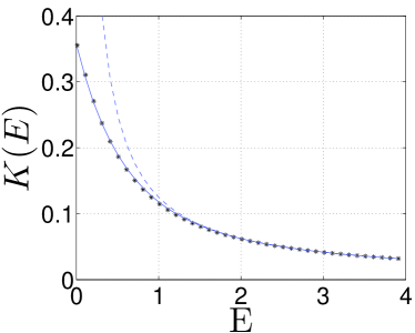
Figure 8: The function $\mathcal{K}(E)$ calculated numerically (symbols). The solid and dashed lines are our approximation Eq.(35) and the asymptotic $1/(8E)$ respectively.

The inverse localization length is related to the counting function by the Thouless relation, namely Eq(19) of thouless . Note that the subsequent formulas there are confused as far as units are concerned. In order to remedy this confusion we define

$$\mathcal{K}(E)\ \ =\ \ \int\frac{\mathcal{N}(z)-\mathcal{N}_{0}(z)}{E-z}dz$$ (32)

and write the Thouless relation as follows:

$$\gamma\ =\ \left(\frac{\text{Var}(v_{n})}{2w_{0}^{2}}\right)^{1/3}\mathcal{K}\left[\left(2\frac{[\text{Var}(v_{n})]^{2}}{w_{0}}\right)^{-1/3}\,\lambda\right]\ \ \ \ \ \ \ \ \$$ (33)

For large $E$ one obtains ${\mathcal{K}(E)\approx 1/(8E)}$ and the Born approximation is recovered:

$$\gamma\ \ =\ \ \frac{\text{Var}(v_{n})}{8w_{0}\,\lambda}\ \ =\ \ \frac{\text{Var}(v_{n})}{8w_{0}^{2}\,k^{2}}$$ (34)

For practical purpose we find that an excellent approximation for any ${E>0}$ is provided by

$$\mathcal{K}(E)\ \ \approx\ \ \left[1-\exp\left(-\frac{E}{E_{0}}\right)\right]\frac{1}{8\,E}$$ (35)

where $E_{0}=0.35$. See Fig.8 for demonstration.

References

- (1)
- (2) S. Lepri, R. Livi, & A. Politi, Phys. Rep. 377, 1 (2003).
- (3) A. Dhar, Adv. Phys. 57, 457 (2008).
- (4) N. Li, J. Ren, L. Wang, G. Zhang, P. Hänggi, and B. Li, Rev. Mod. Phys. 84, 1045 (2012).
- (5) C.W. Chang, D. Okawa, H. Garcia, A. Majumdar, A. Zettl, Phys. Rev. Lett, 101, 075903 (2008).
- (6) D.L. Nika, S. Ghosh, E. P. Pokatilov, and A. A. Balandin, Appl. Phys. Lett. 94, 203103 (2009).
- (7) G. Zhang, B. Li, NanoScale 2, 1058 (2010).
- (8) H. Li, T. Kottos, B. Shapiro, Phys. Rev. E 91, 042125 (2015).
- (9) M. Schmidt, T. Kottos, B. Shapiro, Phys. Rev. E 88, 022126 (2013).
- (10) A. Dhar, Phys. Rev. Lett. 86, 5882 (2001).
- (11) S. Liu, X. Xu, R. Xie, G. Zhang, B. Li, Euro. Phys. J. B 85, 337 (2012).
- (12) A. Dhar, J.L. Lebowitz, Phys. Rev. Lett. 100, 134301 (2008).
- (13) L. W. Lee, A. Dhar, Phys. Rev. Lett. 95, 094302 (2005).
- (14) D. Roy, A. Dhar, Phys. Rev. E 78, 051112 (2008).
- (15) B. Li, H. Zhao, B. Hu, Phys. Rev. Lett. 86, 63 (2001).
- (16) A. Kundu, A. Chaudhuri, D. Roy, A. Dhar, J.L. Lebowitz, H. Spohn, Europhys. Lett. 90, 40001 (2010).
- (17) A. Chaudhuri, A. Kundu, D. Roy, A. Dhar, J.L. Lebowitz, H. Spohn, Phys. Rev. B 81, 064301 (2010).
- (18) J.D. Bodyfelt, M. C. Zheng, R. Fleischmann, T. Kottos, Phys. Rev. E 87, 020101(R) (2013)
- (19) B. Derrida and E. Gardner, J. Physique 45, 1283 (1984).
- (20) A.A. Abrikosov, Solid State Communications 37, 997 (1981)
- (21) B. Shapiro, Phys. Rev. B 34, R4394 (1986)
- (22) F.M. Izrailev, A.A. Krokhin, N.M. Makarov, Physics Reports 512, 125 (2012).
- (23) Y. Dubi, M. Di Ventra, Phys. Rev. E 79, 042101 (2009).
- (24) B.I. Halperin, Phys. Rev. 139, A104 (1965).
- (25) D.J. Thouless, J. Phys. C 5, 77 (1972).
- (26) V. Gurarie, G. Refael, J.T. Chalker, Phys. Rev. Lett. 101, 170407 (2008).
- (27) T.A.L. Ziman, Phys. Rev. Lett. 49, 337 (1982).
- (28) Given an eigenstate we define . The normalization is such that . The participation number PN is a measure for the number of sites that are occupied by the eigenstate.