On Clustering Time Series Using Euclidean Distance and Pearson Correlation

Abstract

For time series comparisons, it has often been observed that z-score normalized Euclidean distances far outperform the unnormalized variant. In this paper we show that a z-score normalized, squared Euclidean Distance is, in fact, equal to a distance based on Pearson Correlation. This has profound impact on many distance-based classification or clustering methods. In addition to this theoretically sound result we also show that the often used k-Means algorithm formally needs a modification to keep the interpretation as Pearson correlation strictly valid. Experimental results demonstrate that in many cases the standard k-Means algorithm generally produces the same results.

1 Introduction

In the KD-Nuggets poll of July 2007 for the most frequently analyzed type of data, time series data was voted on the second place. It is therefore not surprising, that a large number of papers with algorithms to cluster, classify, segment or index time series have been published in recent years. For all these tasks, measures to compare time series are needed, and quite a number of measures have been proposed (cf. [1]). Among these measures, the Euclidean distance is by far the most frequently used distance measure (although many more sophisticated measures exist) [1] with applications in finance [2], medicine [3] or electric power load-forecast [4], to mention only a few. However, many authors then realize that normalizing the Euclidean distance before applying standard machine learning algorithms hugely improves their results.

In this paper, we closer investigate the popular combination of clustering time series data together with a normalized Euclidean distance. The most commonly used learning method for clustering tasks is the k-Means algorithm [5]. We show that a z-score normalized squared Euclidean distance is actually equal (up to a constant factor) to a distance based on the Pearson correlation coefficient. This oberservation allows for standard learning methods based on a Euclidean distance to use a Pearson correlation coefficient by simply performing an appropriate normalization of the input data. This finding applies to all learning methods which are based solely on a distance metric and do not perform subsequent operations, such as a weighted average. Therefore reasonably simple methods such as k Nearest Neighbor and hierarchical clustering but also more complex learning algorithms based on e.g. kernels can be converted into using a Pearson correlation coefficient without actually touching the underlying algorithm itself.

In order to show how this affects algorithms that do perform additional e.g. averaging operations, we chose the often used k-Means algorithm which requires a modification of the underlying clustering procedure to work correctly. Experiments indicate, however, that the difference between the standard Euclidean-based k-Means and the Pearson-based k-Means do not have a high impact on the results, therefore indicating that even in such cases a simple data preprocessing can turn an algorithm using a Euclidean distance into its equivalent based on a Pearson correlation coefficient.

Our paper is organized as follows. In section 2 we briefly recap distances for time series. Afterwards we show that a properly normalized Euclidean distance is equivalent to a distance based on the Pearson correlation coefficient. After this theoretically sound result we quickly review k-means and the required modifications to operate on a Pearson correlation coefficient. In section 6 we perform experiments that demonstrate the (small) difference in behaviour for standard k-Means with preprocessed inputs and the modified version.

2 Measuring Time Series Similarity

In this section, we briefly review the Euclidean distance which is frequently used by data miners and a distance based on Pearson Correlation which is more often used to measure the strength and direction of a linear dependency between time series. Suppose we have two time series $r$ and $s$, consisting of $T$ samples each $r=(r_{1},r_{2},...,r_{T})\in\mbox{\bf R}^{T}$.

Euclidean Distance.

The squared Euclidean distance between two time series $r$ and $s$ is given by:

$$d_{E}(r,s)=\sum_{t=1}^{T}(r_{t}-s_{t})^{2}$$ (1)

The Euclidean distance is a metric, that is, if $r$ and $s$ have zero distance, then $r=s$ holds. For time series analysis, it is often recommended to normalize the time series either globally or locally to tolerate vastly different ranges [1].

Pearson Correlation Coefficient.

The Pearson correlation coefficient measures the correlation $\varrho$ between two random variables $X$ and $Y$:

$$\varrho_{X,Y}=\frac{E[(X-\mu_{X})(Y-\mu_{Y})]}{\sigma_{X}\sigma_{Y}}$$ (2)

where $\mu_{X}$ denotes the mean and $\sigma_{X}$ the standard deviation of $X$. We obtain a value of $+/-1$ if $X$ and $Y$ are perfectly (anti-) correlated and a value of $\approx 0$ if they are uncorrelated.

In order to use the Pearson correlation coefficient as a distance measure for time series it is desirable to generate low distance values for positively correlated (and thus similar) series. The Pearson distance is therefore defined as

$$d_{P}(r,s)=1-\varrho_{r,s}=1-\frac{\frac{1}{T}\sum_{t=1}^{T}(r_{t}-\mu_{r})(s_{t}-\mu_{s})}{\sigma_{r}\sigma_{s}}$$ (3)

such that $0\leq d_{P}(r,s)\leq 2$. We obtain a perfect match (zero distance) for time series $r$ and $s$ if there is an $\alpha,\beta\in\mbox{\bf R}$ with $\beta>0$ such that $r_{i}=\alpha+\beta s_{i}$ for all $1\leq i\leq T$. Thus, a clustering algorithm using this distance measure is invariant with respect to shift and scaling of the time series.

3 Normalized Euclidean Distance vs. Pearson Coefficient

In this section we show that a squared Euclidean Distance can be expressed by a Pearson Coefficient as long as the Euclidean Distance is normalized appropriately (to zero mean and unit variance). Note that this transformation is applied and recommended by many authors as noted in [1].

We consider the squared Euclidean distance as given in equation 1:

$$d_{E}(r,s) = \sum_{t=1}^{T}(r_{t}-s_{t})^{2}$$

$$= \sum_{t=1}^{T}r_{t}^{2}-2\sum_{t=1}^{T}r_{t}s_{t}+\sum_{t=1}^{T}s_{t}^{2}$$

$$= \underbrace{\sum_{t=1}^{T}(r_{t}-0)^{2}}_{(a)}-2\sum_{t=1}^{T}r_{t}s_{t}+\underbrace{\sum_{t=1}^{T}(s_{t}-0)^{2}}_{(b)}$$

the first resp. third part (a/b) of this equation reflect $T$ times the standard deviation of series $r$ resp. $s$ assuming that the series are normalized to have a mean $\mu_{r/s}=0$. Assuming that the normalization also ensures both standard deviations be $\sigma_{r/s}=1$ (resulting in terms (a) and (b) to be equal to $T$), we can simplify the above equation to:

$$d_{E}(r_{\mbox{\footnotesize norm}},s_{\mbox{\footnotesize norm}}) = 2\cdot T-2\sum_{t=1}^{T}r_{\mbox{\footnotesize norm},t}\cdot s_{\mbox{\footnotesize norm},t}$$

$$= 2\cdot T\left(1-\frac{\frac{1}{T}\sum_{t=1}^{T}(r_{\mbox{\footnotesize norm},t}-0)(s_{\mbox{\footnotesize norm},t}-0)}{1\cdot 1}\right)$$

$$= 2\cdot T\cdot d_{P}(r_{\mbox{\footnotesize norm}},s_{\mbox{\footnotesize norm}})$$

Therefore the Euclidean distance of two normalized series is exactly equal to the Pearson Coefficient, bare a constant factor of $2T$.

The equivalence of normalized Euclidean distance and Pearson Coefficient is particularly interesting, since many published results on using Euclidean distance functions for time series similarities come to the finding that a normalization of the original time series is crucial. As the above shows, these authors may in fact end up simulating a Pearson correlation coefficient or a multiple of it.

This result can be applied to any learning algorithm which relies solely on the distance measures but does not perform additional computations based on the distance measure, such as averaging or other aggregation operations. This is the case for many simple algorithms such as k Nearest Neighbor and hierarchical clustering but also applies to more sophisticated learning methods such as kernel methods.

However, some algorithms, such as the prominent k-Means algorithm do perform a subsequent (sometimes weighted) averaging of the training instances to compute new cluster centers. Here we can not simply apply the above and – by normalizing the input data – introduce a different underlying distance measure. However, since quite often only a ranking of patterns with respect to the underlying distance function is actually used it would be interesting to see if and how this observation can be used to apply also to such learning algorithms without actually adjusting the entire algorithm. In the following section we will show how this works for the well known and often used $k$-Means Clustering algorithm.

4 Brief Review of $k$-Means

The $k$-Means algorithm [5] is one of the most popular clustering algorithms. It encodes a partition into $k$ clusters by means of $k$ prototypical data points $p_{i}$, $1\leq i\leq k$, and assigns every record $x_{j}$, $1\leq j\leq n$, to its closest prototype. It minimizes the objective function

$$J=\sum_{j=1}^{n}\sum_{i=1}^{c}u_{i,j}\cdot d_{i,j}$$ (4)

where $u_{i,j}\in\{0,1\}$ encodes the partition ($u_{i,j}=1$ iff record $j$ is assigned to cluster/prototype $i$) and $d_{i,j}$ is the distance between record $j$ and prototype $i$. The classical $k$-Means uses the squared Euclidean distance as $d_{i,j}=d_{E}(x_{j},p_{i})$.

In the batch version of $k$-Means the prototypes and cluster memberships are updated alternatingly to minimize the objective function (4). In each step, one part of the parameters (cluster memberships resp. cluster centers) is kept fixed while the other is optimized. Hence the two phases of the algorithm first assume that the prototypes are optimal and determine how we can then minimize $J$ wrt the membership degrees. Since we allow values of 0 and 1 only for $u_{i,j}$, we minimize $J$ by assigning a record to the closest prototype (with the smallest distance):

$$u_{i,j}=\left\{\begin{array}[]{ll}1&\mbox{if~{}}d_{i,j}=\min_{k}d_{k,j}\\ 0&\mbox{otherwise}\\ \end{array}\right.$$ (5)

Afterwards, assuming that the memberships are optimal, we then find the optimal position of the prototypes. The answer for this question can be obtained by solving the (partial) derivatives of $\partial J/\partial p_{i}=0$ for $p_{i}$ (necessary condition for $J$ having a minimum). In case of an Euclidean distance, the optimal position is then the mean of all data objects assigned to cluster $p_{i}$:

$$p_{i}=\frac{\sum_{j=1}^{n}\sum_{i=1}^{c}u_{i,j}x_{j}}{\sum_{i=1}^{c}u_{i,j}}$$ (6)

where the denominator represents the number of data objects assigned to prototype $p_{i}$. The resulting $k$-Means algorithm is shown below:

initialize prototypes (i.e. randomly draw from input data)

repeat

update memberships using eq. (5)

update prototypes using eq. (6)

until convergence

5 k-Means Clustering using Pearson Correlation

The $k$-Means algorithm has its name from the prototype update (6), which re-adjusts each prototype to the mean of its assigned data objects. The reason why the mean delivers the optimal prototypes is due to the use of the Euclidean distance measure – if we change the distance measure in (4), we have to check carefully if the update equations need to be changed, too. We have seen in section 3 that the Euclidean distances becomes the Pearson Coefficient (up to a constant factor) if the vectors are normalized. But if the distances are actually identical, should not the prototype update also be the same?

The equivalence $2d_{E}(r,s)=d_{P}(r,s)$ holds only for normalized time series $r$ and $s$. To avoid constantly normalizing time series in the Pearson Coefficient (2), we transform all series during preprocessing, that is, we replace $r_{i}=(r_{i,t})_{1\leq t\leq T}$ by $\hat{r}_{i}=(\hat{r}_{i,t})_{1\leq t\leq T}$ with $\hat{r}_{i,t}=\frac{r_{i,t}-\mu_{r}}{\sigma_{r}}$, $1\leq t\leq T,1\leq i\leq n$. But in the k-Means objective function (4) the arguments of the distance function are always pairs of data object and prototype. While our time series data has been normalized at the beginning, this does not necessarily hold for the prototypes.

If the prototypes are calculated as the mean of normalized time series (standard k-Means), the prototypes will also have zero mean, but a unit variance can not be guaranteed. Once the prototypes have been calculated, their variance is no longer 1 and the equivalence no longer holds. Therefore, in order to stick to the Pearson Coefficient, we must include an additional constraint on the prototypes while minimizing (4).

We use Lagrange multipliers $\lambda_{i}$, one for each cluster, to incorporate this constraint in the objective function. So we arrive at:

$$J_{P}=\sum_{i=1}^{n}\sum_{j=1}^{c}u_{i,j}(1-x_{j}^{\top}p_{i})+\sum_{i=1}^{n}\lambda_{i}(\|p_{i}\|^{2}-1)$$ (7)

As with classical k-Means we arrive at the new prototype update equations by solving $\partial J/\partial p_{i}=0$ for the prototype $p_{i}$ (see appendix for the derivation):

$$p_{i,t}=\frac{1}{\sqrt{\sum_{t=1}^{T}\left(\sum_{j=1}^{n}u_{i,j}x_{j,t}\right)^{2}}}\sum_{j=1}^{n}u_{i,j}x_{j,t}$$ (8)

This corresponds to a normalization of the usually obtained prototypes to guarantee the constraint of unit variance. Note that formally, due to a division by zero, it is not possible to include constant time series when using Pearson distance (because normalization leads to $x_{j,t}=0$ for all $t$ and we would have a division by zero).

We now have a version of k-Means which uses the Pearson correlation coefficient as underlying distance measure. But does the difference between the different update equations 8 and 6 really matter? In the following we will show via a number of experiments that the influence of this optimization is small.

6 Experimental Evaluation

The goal of the experimental evaluation is twofold. The k-Means algorithm has been used frequently with z-score normalized time series in the literature. We have seen that in this case a semantically sound solution would require the modifications of section 5. Do we obtain “wrong” results when using standard k-Means? Will the corrected version with normalization yield different results at all? And if so, how much will the resulting cluster differ from each other on the kind of data used typically in the literature.

6.1 Artificial Data: Playing Devils Advocate

We expect that the influence of the additional normalization step on the results is rather small. An unnormalized prototype $p_{i}$ in k-Means is now normalized by an additonal factor of $\alpha_{i}=1/\|p_{i}\|$ in the modified k-Means. The distances of all data objects to this prototype miss this factor. However, if the factors $\alpha_{i}$ are approximately the same for all prototoypes $p_{i}$, we make the same relative error with all clusters and the rank of a cluster with respect to the distance does not change. Since $k$-Means assigns each data object to the top-ranked cluster, the differences in the distances then do not influence the prototype assignment. Note also that this (presumably small) error does not propagate further, since we re-compute the average again from the normalized input data during each iteration of the algorithm.

Before presenting some experimental results, let us first discuss under what circumstances a difference between both versions of k-Means may occur. Let us assume for the sake of simplicity that a cluster consists of two time series $r$ and $s$ only. Then the prototype of standard k-Means is $p=\frac{r+s}{2}$. Since the mean of $p$ will then also be zero, the variance of the new prototype $p$ is identical to its squared Euclidean norm $\|p-\bar{p}\|^{2}=\|p-0\|^{2}=\|p\|^{2}$, so we have:

$$\|p\|^{2}=\left\|\frac{r+s}{2}\right\|^{2}=\frac{1}{4}\left(\|r\|^{2}+\|s\|^{2}+2r^{\top}s\right)$$

From the Cauchy Schwarz inequality and the z-score normalization of $r$ and $s$ (in particular $\|r\|=\|s\|=1$) we conclude $r^{\top}s\in[-1,1]$ since $(r^{\top}s)^{2}\leq\|r\|^{2}\cdot\|s\|^{2}=1\cdot 1$. Apparently $\|p\|$ becomes maximal, if $r^{\top}s$ or equivalently the Pearson Coefficient becomes maximal. The new prototype $p$ will have unit variance if and only if $r$ and $s$ correlate perfectly (Pearson Coefficient of 1). If the new prototype $p$ is build from data that is not perfectly correlated, its norm $\|p\|$ will be smaller than one – the worse the correlation, the smaller the norm of $p$. As a consequence, for any subsequent distance calculation $d_{P}(r,p)=2-2r^{\top}p$ we obtain larger distance values compared to what would be obtained from a correctly normalized prototype $d_{P}(r,p)=2-2r^{\top}\frac{p}{\|p\|}$ (since $\|p\|<1$).

As already mentioned, in order to have influence on the ranking of the clusters (based on the prototype-distance), the prototype’s norm must differ within the clusters. This may easily happen if, for instance, the amount of noise is not the same in all clusters: A set of linearly increasing time series without any noise correlates perfectly, but by adding random noise to the series the Pearson coefficient approaches 0 when the amplitude of the noise is continuosly increased.

To demonstrate the relevance of these theoretical considerations we construct an artificial test data set. It will consist of two clusters (100 time series each) and a few additional time series serving as probes that demonstrate the different behavior of the two algorithms.

The test set contains a cluster of linearly increasing time series $r_{I}=(0,1,2,..,29,30,31)$ as well as a cluster of linearly decreasing time series $r_{D}=(31,30,29,...,2,1,0)$, 100 series per each cluster. We add Gaussian noise with $\sigma=30$ and $\sigma=10$ to the samples, that is, the data with increasing trend is more noisy than the data with decreasing trend. Finally, we add another 10 time series that equally belong to both clusters as they consist of a linearly increasing and a linearly decreasing portion: $r_{M}=(16,15,14,13,..2,1,0,1,2,..,13,14,15)$. The Pearson correlation between $r_{M}$ and $r_{I}$ as well as $r_{D}$ is identical, therefore our expectation is that – after adding some Gaussian noise with $\sigma=10$ to this group of time series – on average half of them is assigned to each cluster. For the experiment we want to concentrate on how the small group of these “probe series” is distributed among both clusters. The data from each group of time series is shown in figure 1.

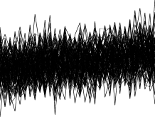
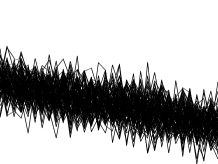
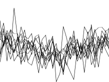
Figure 1: Groups of time series in the test data set.

To reduce the influence of random effects, we initialize the clusters with linearly increasing and decreasing series (but the prototypes do not stick to this initialization due to the noise in the data). Clustering the z-score normalized data with standard k-Means finally arrives at prototypes with a norm of $0.07$ (increasing cluster) and $0.31$ (decreasing cluster) approximately. Instead of the expected tie situation, all the probing series but one are assigned to the cluster representing the increasing series (9:1). If we include the normalization step for the Pearson-based k-Means, we obtain an equal distribution among both clusters (5:5).

Given that the semantics of clustering z-score normalized time series is so close to clustering via Pearson correlation, this example clearly indicates that we may obtain counterintuitive partitions when using standard k-Means. Clusters of poorly correlating data greedily absorb more data than it would be justified by the Pearson correlation. This undesired bias is removed by the properly modified version of k-Means. Still, the chosen example is artificial and rather drastic - the question remains how big the influence of this issue really is in practice.

6.2 Real World Datasets

In order to demonstrate this on real world data sets, we use the time series data sets for clustering tasks, available online [6]. For each data set we use the number of classes as the number of clusters and run each experiment five times with different random selections of initial prototypes for each run of k-Means. During each run we use the same vectors as initial prototypes for the different types of algorithms to avoid problems with the unfamously instable k-Means algorithm. In order to compare the result to the natural instability of k-Means, we run a third experiment with a different random initialization. That is, for each data set we do:

1. set the number of clusters to the number of classes,

2. normalize each time series (row) to have $\mu=0$ and $\sigma=1$,

3. create a clustering $\mathcal{C}_{1}$ using the classical k-Means algorithm with the Euclidean distance (no normalization),

4. create a clustering $\mathcal{C}_{2}$ using a k-Means algorithm using the Euclidean distance but prototype update equation (8) with normalization after each iteration,

5. create a clustering $\mathcal{C}_{3}$ using a k-Means algorithm using the Euclidean distance and no normalization of the prototypes using a different (randomly chosen) initialization of the prototypes.

We then compute the average entropy over five runs of the clustering $\mathcal{C}_{1}$ with respect to $\mathcal{C}_{2}$ (called $E_{pear}$) and $\mathcal{C}_{1}$ with respect to $\mathcal{C}_{3}$ (denoted by $E_{random}$). The entropy measures are composed of the weighted average over the entropy of all clusters in one clustering using the cluster indices of the other clustering as class labels. $E_{pear}$ therefore measures the difference between a clustering achieved with the correctly modified k-Means algorithm and its lazy version where we only normalize the input data but refrain from normalizing the prototypes. $E_{random}$ shows the difference between two runs of k-Means with the same setting but different initalizations to illustrate the natural, internal instability of k-Means. The hypothesis would be that $E_{pear}$ should be zero or at least substantially below $E_{random}$, that is, using the Pearson correlation coefficient should not have a worse influence on k-Means than different initializations. Table 1 shows the results. We show the name of the dataset and the number of clusters in the first two columns. Length and number of time series in the training data are listed in columns 3 and 4. The following four columns show minimum resp. maximum value over our five experiments for the two entropies.

Table 1: Experimental results using different version of k-Means. See text for details.

Name #clusters #length #size $E_{pear}$ $E_{random}$ min max min max Synthetic Control 6 60 300 0,32 0,36 0,41 0,62 Gun Point 2 150 50 0,0 0,0 0,0 0,59 CBF 3 128 30 0,0 0,0 0,30 0,85 Face (All) 14 131 560 0,03 0,16 1,12 1,53 OSU Leaf 6 427 200 0,06 0,26 0,93 1,25 Swedish Leaf 15 128 500 0,0 0,03 0,83 1,09 50Words 50 270 450 0,0 0,05 1,17 1,27 Trace 4 275 100 0,0 0,0 0,50 0,67 Two Patterns 4 128 1000 0,03 0,11 0,86 1,41 Wafer 2 152 1000 0,0 0,0 0,0 0,0 Face (Four) 4 350 24 0,0 0,0 0,62 1,19 Lightning-2 2 637 60 0,0 0,0 0,0 0,71 Lightning-7 7 319 70 0,0 0,07 0,35 0,99 ECG 2 96 100 0,0 0,0 0,0 0,55 Adiac 37 176 390 0,0 0,0 0,89 1,23 Yoga 2 426 399 0,0 0,0 0,0 0,76

As one can see clearly in this table, the difference between running classical k-Means on z-score normalized input and the “correct” version with prototype-normalization is small. The clusterings are the same ($E_{pear}=0$) when k-Means is reasonably stable ($E_{random}\approx 0$), that is an underlying reasonably well defined clustering of the data exists (Gun Point and Wafer are good examples for this effect). In case of an unstable k-Means, also the normalization of the prototypes (or the lack of it) may change the outcome slightly but will never have the same impact as a different initialization of the same algorithm on the same data. Strong evidence for this effect can be seen by $\max\{E_{pear}\}\leq\min\{E_{random}\}$ in all case. Note how in many case even an unstable classic k-Means does not indicate any difference between the prototype normalized and unnormalized versions, however. Gun Point, CBF, Trace, and Face-Four among others are good examples for this effect.

From these experiments it seems safe to conclude that one can simulate k-Means based on Pearson correlation coefficients as similarity metric by simply normalizing the input data without changing the normal (e.g. Euclidean distance based) algorithm at all. It is, of course, even easier to apply the discussed properties to classification or clustering algorithms which do not need subsequent averaging steps, such as k-Nearest Neighbor, hierarchical clustering, Kernel Methods etc. In these cases a distance function using Pearson correlations can be perfectly emulated by simply normalizing the input data appropriately and then using the existing implementation based on the Euclidean distance.

7 Conclusion

We have shown that the squared Euclidean distance on z-score normalized vectors is equivalent to the inverse of the Pearson Correlation coefficient up to a constant factor. This result is especially of interest for a number of time series clustering experiments where Euclidean distances are applied to normalized data as it shows that the authors in fact were often using something close to or equivalent to the Pearson correlation coefficient.

We have also experimentally demonstrated that the standard k-Means clustering algorithm without proper normalization of the prototypes still performs similar to the correct version, enabling the use of standard k-Means implementations without modification to compute clusterings using Pearson coefficients. Algorithms without “internal” computations, such as k-Nearest Neighbor or hierarchical clustering can make use of the theoretical proof provided in this paper and be applied without any further modifications, of course.

Appendix 0.A Update Equation for Pearson Distance

The derivation with respect to the reference time series $p_{i}$ at time $t$ is

$$\frac{\partial J}{\partial p_{i,t}}=2\lambda_{i}p_{i,t}-\sum_{j=1}^{n}u_{i,j}x_{i,t}$$

Setting the derivative to zero (necessary condition for minimum) yields

$$p_{i,t}=\frac{1}{2\lambda_{i}}\sum_{j=1}^{n}u_{i,j}x_{j,t}$$ (9)

Replacing $p_{i,t}$ in the normalization constraint (guaranteed by Lagrange multiplier) yields

$$1=\|p_{i}\|^{2}=\sum_{t=1}^{T}p_{i,t}^{2}=\frac{1}{4\lambda_{i}^{2}}\sum_{t=1}^{T}\left(\sum_{j=1}^{n}u_{i,j}x_{j,t}\right)^{2}$$

or

$$\lambda_{i}=\frac{1}{2}\sqrt{\sum_{t=1}^{T}\left(\sum_{j=1}^{n}u_{i,j}x_{j,t}\right)^{2}}$$

Inserting this expression into (9) gives us finally the following update equation

$$p_{i,t}=\frac{1}{\sqrt{\sum_{t=1}^{T}\left(\sum_{j=1}^{n}u_{i,j}x_{j,t}\right)^{2}}}\sum_{j=1}^{n}u_{i,j}x_{j,t}$$

References

- [1] Keogh, E., Kasetty, S.: On the Need for Time Series Data Mining Benchmarks: A Survey and Empirical Demonstration. Data Mining and Knowledge Discovery 7(4) (2003) 349–371
- [2] Gavrilov, M., Anguelov, D., Indyk, P., Motwani, R.: Mining the stock market: which measure is best? In: Proc. 6th ACM SIGKDD Int. Conf. on Knowledge Discovery and Data Mining. (2000) 487–496
- [3] Caraça-Valente, J.P., López-Chavarrías, I.: Discovering similar patterns in time series. In: Proc. 6th ACM SIGKDD Int. Conf. on Knowledge Discovery and Data Mining. (2000) 497 – 505
- [4] Ruzic, S., Vuckovic, A., Nikolic, N.: Weather sensitive method for short term load forecasting in Electric Power Utility of Serbia. IEEE Transactions on Power Systems 18(4) (2003) 1581–1586
- [5] McQueen, J.B.: Some methods of classification and analysis of multivariate observations. In: Proc. of 5th Berkeley Symp. on Mathematical Statistics and Probability. (1967) 281–297
- [6] Keogh, E., Xi, X., Wei, L., Ratanamahatana, C.A.: The UCR Time Series Classification/Clustering Homepage. www.cs.ucr.edu/~eamonn/time_series_data/ (2006)