Hydrodynamic fluctuations and dissipation in an integrated dynamical model

Abstract

We develop a new integrated dynamical model to investigate the effects of the hydrodynamic fluctuations on observables in high-energy nuclear collisions. We implement hydrodynamic fluctuations in a fully 3-D dynamical model consisting of the hydrodynamic initialization models of the Monte-Carlo Kharzeev-Levin-Nardi model, causal dissipative hydrodynamics and the subsequent hadronic cascades. By analyzing the hadron distributions obtained by massive event-by-event simulations with both of hydrodynamic fluctuations and initial-state fluctuations, we discuss the effects of hydrodynamic fluctuations on the flow harmonics, $v_{n}$ and their fluctuations.

1 Introduction

In high-energy nuclear collisions, initial-state fluctuations are the major origin of event-by-event fluctuations observed in the higher-order azimuthal anisotropies $v_{n}$ of the observed hadrons. Since the hydrodynamic response of the matter converts the initial spatial anisotropies to the final momentum anisotropies, we can extract transport properties of the created matter, such as viscosity and relaxation times, by comparing the initial-state fluctuations and the final observables. However the initial-state fluctuations are not the only source of the event-by-event fluctuations [1]. For example, hydrodynamic fluctuations generate additional flow fluctuations during the hydrodynamic evolution of the matter. Hydrodynamic fluctuations are the thermal fluctuations of the hydrodynamic fields whose power is related to transport coefficients through the fluctuation-dissipation relation (FDR) [2]. To precisely determine the transport properties of the matter, we need to quantify the effects from the hydrodynamic fluctuations on the observables such as the flow coefficients $v_{n}$. We implement hydrodynamic fluctuations into our dynamical model of high-energy nuclear collisions to study the effects.

2 Integrated dynamical model with hydrodynamic fluctuations

We use an extended version of an integrated dynamical model [3] consisting of four parts. First, event-by-event initial conditions are generated using the Monte-Carlo Kharzeev-Levin-Nardi (MC-KLN) model [4]. Subsequent hydrodynamic expansion is calculated using newly developed codes of the second-order relativistic fluctuating hydrodynamics, namely viscous hydrodynamics with hydrodynamic fluctuations. Then we sample hadrons on the isothermal hypersurface at the temperature of 155 MeV using the Cooper-Frye formula [5] including the viscous correction of phase-space distribution $\delta f$ [6]. Finally we perform hadronic cascades using JAM [7] to obtain hadron spectra.

In our hydrodynamic calculations the time evolution of the created matter is solved in the $\tau$-$\eta_{s}$ coordinates: ($\tau$, $\eta_{s}$, $\bm{x}_{\perp}$) where $t=\tau\cosh\eta_{s}$ and $z=\tau\sinh\eta_{s}$. An essential part of hydrodynamic equations is the conservation law of the energy-momentum tensor:

$$\bar{\partial}_{\mu}T^{\mu\nu} =0, T^{\mu\nu} =eu^{\mu}u^{\nu}-P\Delta^{\mu\nu}+\pi^{\mu\nu},$$ (1)

where $\bar{\partial}_{\mu}$ is the covariant derivative, and $e$, $P$ and $\pi^{\mu\nu}$ are the energy density, the equilibrium pressure and the shear stress, respectively. The bulk pressure is not considered here. The Landau frame is adopted for a fluid velocity $u^{\mu}$ ($u_{\mu}u^{\mu}=1$), where $T^{\mu}{}_{\nu}u^{\nu}=eu^{\mu}$. Here the signs of metric tensor $g_{\mu\nu}$ are $(+,-,-,-)$. The tensor $\Delta^{\mu\nu}=g^{\mu\nu}-u^{\mu}u^{\nu}$ is the projector onto the space of four-vectors transverse to the flow velocity. For the equation of state (EoS), $P(e)$, we adopt $s95p$-v1.1 [8] which smoothly connects a lattice EoS at high temperature and a hadron gas EoS at low temperature. For the evolution of the shear stress, the following constitutive equation is used:

$$\tau_{\pi}\Delta^{\mu\nu}{}_{\alpha\beta}u^{\lambda}\bar{\partial}_{\lambda}\pi^{\alpha\beta}+\pi^{\mu\nu}[1+(4/3)\tau_{\pi}\bar{\partial}_{\lambda}u^{\lambda}] =2\eta\Delta^{\mu\nu}{}_{\alpha\beta}\bar{\partial}^{\alpha}u^{\beta}+\xi^{\mu\nu},$$ (2)

where $\Delta^{\mu\nu}{}_{\alpha\beta}=\frac{1}{2}(\Delta^{\mu}{}_{\alpha}\Delta^{\nu}{}_{\beta}+\Delta^{\mu}{}_{\beta}\Delta^{\nu}{}_{\alpha})-\frac{1}{3}\Delta^{\mu\nu}\Delta_{\alpha\beta}$ is the projector onto the tensor components which are symmetric, traceless and transverse to the flow velocity. In this study, the shear viscosity coefficient $\eta$ is fixed to be the KSS bound: $\eta/s=1/4\pi$ [9]. The relaxation time is chosen as $\tau_{\pi}=3/4\pi T$ [10, 11]. Hydrodynamic fluctuations appear as the term $\xi^{\mu\nu}$ which is the Gaussian white noise with autocorrelations determined by the FDR [12]:

$$\langle\xi^{\mu\nu}(x)\xi^{\alpha\beta}(x^{\prime})\rangle =4T\eta\Delta^{\mu\nu\alpha\beta}\delta^{(4)}(x-x^{\prime}).$$ (3)

Noise values are numerically generated using Gaussian random numbers. The above autocorrelations are diagonalized by considering proper linear combinations of noise components: $\xi^{(i)}$ ($i=1,\dots,5$), so that correlations among different components are disentangled. Then independent noise components $\xi^{(i)}$ are generated as:

$$\xi^{(i)}(\tau,\eta_{s},\bm{x}_{\perp}) =\sqrt{4T\eta\Delta^{(i)}/\tau}\,w_{i}(\tau,\eta_{s},\bm{x}_{\perp}),$$ (4)

where $w_{i}(x)$ are the normal Gaussian noise fields, and $\Delta^{(i)}$ are coefficients coming from the projector. The Jacobian $1/\tau=1/\sqrt{-g}$ for the $\tau$-$\eta_{s}$ coordinates comes from a coordinate transform of the delta function.

Here we introduce a coarse-graining scale or a cutoff length scale of the hydrodynamic fluctuations. The hydrodynamic description of physical systems has always a lower-bound scale of the description where the assumption of the local equilibrium becomes invalid. If hydrodynamic fluctuations with arbitrarily small wavelength are considered, the magnitude of fluctuations diverges such that the stress tensor becomes unphysically large and breaks calculations. Therefore we introduce a coarse-graining scale of the hydrodynamic fluctuations by replacing the normal noise fields $w_{i}(x)$ in (4) with smeared ones $w^{\prime}_{i}(x)$:

$$w^{\prime}_{i}(\tau,\eta_{s},\bm{x}_{\perp}) =\int d\eta_{s}^{\prime}d^{2}x^{\prime}_{\perp}\frac{1}{\sqrt{(2\pi)^{3}}\sigma_{\eta}\sigma_{\perp}^{2}}\exp\left(-\frac{(\eta_{s}-\eta_{s}^{\prime})^{2}}{2\sigma_{\eta}^{2}}-\frac{(\bm{x}_{\perp}-\bm{x}^{\prime}_{\perp})^{2}}{2\sigma_{\perp}^{2}}\right)w_{i}(\tau,\eta_{s}^{\prime},\bm{x}^{\prime}_{\perp}).$$ (5)

For this study, we choose smearing scales as $\sigma_{\perp}=1\;\textrm{fm}$, and $\sigma_{\eta}=1$.

3 Results

To quantify the effects of hydrodynamic fluctuations on observables, we perform event-by-event simulations using the integrated dynamical model. For the collision system we consider minimum-bias Au+Au collisions at the collision energy $\sqrt{s_{\mathrm{NN}}}=$ 200 GeV. We consider two types of hydrodynamic calculations: fluctuating hydrodynamics with the shear viscosity and the corresponding hydrodynamic fluctuations, and conventional viscous hydrodynamics without hydrodynamic fluctuations. The initial-state entropy densities are scaled for each type of hydrodynamics to reproduce experimental charged particle multiplicities [13]. For each type of hydrodynamics we perform $10^{5}$ events of hydrodynamic simulations. Then one hundred events of hadronic cascades are performed for each hydrodynamic event, i.e., $10^{5}\times 100=10^{7}$ cascades are performed in total for each type of hydrodynamics.

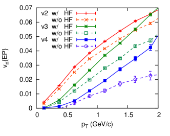
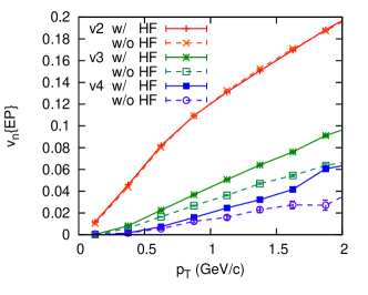
Fig. 1: The $p_{T}$ differential flows of the charged hadrons are shown for central collisions 0-5% (the left panel), and for non-central collisions 20-30% (the right panel). The flow coefficients are calculated using the $\eta$-sub method with two subevents at the pseudorapidity range $1<|\eta|<2.8$. The solid lines are the results from fluctuating hydrodynamics with hydrodynamic fluctuations (HF), and the dashed ones are from conventional viscous hydrodynamics.

In the left panel of Fig. 1, we see increase of the flow harmonics $v_{n}$ in central collisions 0-5% due to hydrodynamic fluctuations. The amount of increase is larger for higher order of the harmonics, which can be understood by the FDR: The effective size of the fluctuations scales as $\xi\propto 1/\sqrt{V}$ since the delta function in the FDR becomes $1/V$ through effective coarse graining in the volume $V$. As a higher order of harmonics corresponds to smaller structures of the created matter, the effects are larger for the higher order.

The right panel of Fig. 1 shows the same results for non-central collisions 20-30%. Unlike the case of the central collisions, the elliptic flows $v_{2}$ are almost identical with each other in both cases, which can be explained by a difference of the origin of elliptic flows. In central collisions, the origin of elliptic flows is dominated by fluctuations. In non-central collisions, there is an additional origin from the collision geometry. Small flow fluctuations caused by hydrodynamic fluctuations around the large geometrical elliptic flow do not change the average magnitude of the flows. Nevertheless the distribution of the flows is changed by hydrodynamic fluctuations. This can be confirmed in Fig. 2 in which the event-by-event distribution of $v_{2}$ in the non-central collisions is broadened by hydrodynamic fluctuations.

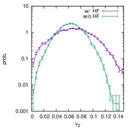
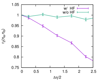
Fig. 2: In the left panel, the event-by-event distributions of the $p_{T}$-integrated $v_{2}$ for non-central collisions 20-30% are shown. The vertical axis indicates the probability density of $v_{n}$. In the right panel, $\eta$-dependent factorization ratio $r_{2}(\eta_{a},\eta_{b})$ proposed in Ref. [14] is shown for non-central collisions. The horizontal axis is $\eta_{a}=\Delta\eta/2$. The rapidity range for $\eta_{b}$ is fixed as $3<\eta_{b}<3.5$.

Another effect caused by hydrodynamic fluctuations is the decorrelation of the flow angles at different rapidities which have a strong correlation due to the initial-state fluctuations from nucleon position distributions. The decorrelations can be caused by several mechanisms [15] including hydrodynamic fluctuations. In the right panel of Fig. 2 we see the decorrelation by hydrodynamic fluctuations. The flow angles are disturbed by the hydrodynamic fluctuations which have short longitudinal correlations due to the FDR.

4 Summary and discussions

Hydrodynamic fluctuations have a non-negligible amount of effects on observables of flow harmonics compared to that of the initial-state fluctuations. In central collisions hydrodynamic fluctuations increase the flow coefficients. The increase is larger in higher order of harmonics as expected from the FDR. In non-central collisions with a large geometrical origin of $v_{2}$, hydrodynamic fluctuations do not change $v_{2}$ of the event-plane method which roughly corresponds to the average of event-by-event $v_{2}$. Nevertheless the distribution of the event-by-event $v_{2}$ is broadened by the fluctuations. Also, hydrodynamic fluctuations contribute to the decorrelation of the flow angles in the longitudinal direction.

The effects of hydrodynamic fluctuations are too large with the current parameter set of the shear viscosity, $\eta/s$, and the cutoff scale of hydrodynamic fluctuations, $\sigma_{\eta}$ and $\sigma_{\perp}$, We need to fix the realistic values of those parameters by scanning the parameters in event-by-event calculations. Also there is room to improve the model by taking into account the corrections of various quantities by the cutoff scale of hydrodynamic fluctuations. For example, transport coefficients should be renormalized for each cutoff scale of hydrodynamic fluctuations [16]. The equation of state, the phasespace distribution of hadrons on the switching hypersurface and even the initial entropy density could be subject to change due to renormalization.

This work was supported by JSPS KAKENHI Grant Numbers 12J08554 (K.M.) and 25400269 (T.H.).

References

- [1] J. I. Kapusta, B. Muller, M. Stephanov, Phys. Rev. C85 (2012) 054906. arXiv:1112.6405, doi:10.1103/PhysRevC.85.054906.
- [2] L. D. Landau, E. M. Lifshitz, Fluid Mechanics, Vol. 6 of Course of Theoretical Physics, Pergamon Press, New York, 1959.
- [3] T. Hirano, P. Huovinen, K. Murase, Y. Nara, Prog. Part. Nucl. Phys. 70 (2013) 108–158. arXiv:1204.5814, doi:10.1016/j.ppnp.2013.02.002.
- [4] H.-J. Drescher, Y. Nara, Phys. Rev. C76 (2007) 041903. arXiv:0707.0249, doi:10.1103/PhysRevC.76.041903.
- [5] F. Cooper, G. Frye, Phys. Rev. D10 (1974) 186. doi:10.1103/PhysRevD.10.186.
- [6] D. Teaney, Phys. Rev. C68 (2003) 034913. arXiv:nucl-th/0301099, doi:10.1103/PhysRevC.68.034913.
- [7] Y. Nara, N. Otuka, A. Ohnishi, K. Niita, S. Chiba, Phys. Rev. C61 (2000) 024901. arXiv:nucl-th/9904059, doi:10.1103/PhysRevC.61.024901.
- [8] P. Huovinen, P. Petreczky, Nucl. Phys. A837 (2010) 26–53. arXiv:0912.2541, doi:10.1016/j.nuclphysa.2010.02.015.
- [9] P. Kovtun, D. T. Son, A. O. Starinets, Phys. Rev. Lett. 94 (2005) 111601. arXiv:hep-th/0405231, doi:10.1103/PhysRevLett.94.111601.
-
[10]
H. Song, Ph.D. thesis, Ohio State U. (2009).
arXiv:0908.3656,
[link].
URL http://inspirehep.net/record/829461/files/arXiv:0908.3656.pdf - [11] R. Baier, P. Romatschke, D. T. Son, A. O. Starinets, M. A. Stephanov, JHEP 04 (2008) 100. arXiv:0712.2451, doi:10.1088/1126-6708/2008/04/100.
- [12] K. Murase, T. Hirano, Unpublished results (2013). arXiv:1304.3243.
- [13] S. S. Adler, et al., Phys. Rev. C69 (2004) 034909. arXiv:nucl-ex/0307022, doi:10.1103/PhysRevC.69.034909.
- [14] V. Khachatryan, et al., Phys. Rev. C92 (3) (2015) 034911. arXiv:1503.01692, doi:10.1103/PhysRevC.92.034911.
- [15] J. Jia, P. Huo, Phys. Rev. C90 (3) (2014) 034915. arXiv:1403.6077, doi:10.1103/PhysRevC.90.034915.
- [16] P. Kovtun, J. Phys. A45 (2012) 473001. arXiv:1205.5040, doi:10.1088/1751-8113/45/47/473001.