Bivariate hierarchical Hermite spline quasi–interpolation

Abstract

Spline quasi–interpolation (QI) is a general and powerful approach for the construction of low cost and accurate approximations of a given function. In order to provide an efficient adaptive approximation scheme in the bivariate setting, we consider quasi–interpolation in hierarchical spline spaces. In particular, we study and experiment the features of the hierarchical extension of the tensor–product formulation of the Hermite BS quasi–interpolation scheme. The convergence properties of this hierarchical operator, suitably defined in terms of truncated hierarchical B–spline bases, are analyzed. A selection of numerical examples is presented to compare the performances of the hierarchical and tensor–product versions of the scheme.

Keywords: B–splines, Hermite quasi–Interpolation, Hierarchical spaces, Truncated hierarchical B–splines.

1 Introduction

Whenever exact interpolation is not suited or not strictly necessary, spline quasi–interpolation (QI) is a valuable and widely appreciated approximation methodology, since QI schemes share locality as common denominator (see e.g., the fundamental papers [2, 14]). This is for instance the case when real–time processing of large data streams is required and the input information on a certain target function $f$ can be dynamically updated (and, consequently, also the spline approximation is dynamically updated). In a very general formulation, a spline quasi–interpolant $Q(f)$ to a given function $f$ can be written as follows,

$$Q(f)(\cdot)\,=\,\sum_{\gamma\in\Gamma}\lambda_{\gamma}(f)\,B_{\gamma}(\cdot),$$ (1)

where $B_{\gamma},\,\gamma\in\Gamma\,,$ denote the B–spline basis (or a suitable extension to the multivariate setting) and $\lambda_{\gamma}\,,\gamma\in\Gamma\,,$ are corresponding linear functionals. Even if different approaches can be considered for defining these functionals, they are usually required to be local, namely,

$$\Lambda_{\gamma}\,:=\,\mathop{\mathrm{supp}}(\lambda_{\gamma})\,\subset\,\Omega\,,\quad\forall\,\gamma\in\Gamma\,,$$ (2)

where $\Omega$ denotes the specific domain of interest. The functionals $\lambda_{\gamma}(f)$ are often defined either as a linear combination of evaluations of $f$ at suitable points or as an appropriate integral of $f$, so that the QI operator exactly reproduces all the polynomials of a certain degree or it is a projector on the space spanned by the B-spline basis (see, e.g., [4, 12, 14, 19]). QIs where the definition of $\lambda_{\gamma}(f)$ also involves derivatives of $f$ are usually called Hermite QIs (see, e.g., [15]).

QI spline schemes capable to deal with data on nonuniform meshes are of great interest because they can be profitably used either for adaptive approximation or data reduction purposes. In the univariate setting, the BS Hermite Quasi–Interpolation operator introduced in [15] defines a robust and accurate scheme with this capability. Its recent tensor–product extension to the bivariate setting [9, 10] preserves the robustness and accuracy of the scheme, but necessarily inherits the grid limits of any tensor–product approach. In order to overcome this problem, suitable extensions of tensor–product spline spaces must be considered.

Examples of adaptive spline constructions that provide local refinement possibility by relaxing the rigidity of tensor–product configurations have been widely investigated, see e.g., [5, 6, 11, 13, 20, 21]. The definition of these classes of adaptive splines pose non-trivial issues related to solid basis constructions, the characterization and understanding of the corresponding spline spaces, as well as the design of reliable and efficient refinement algorithms. The introduction of the truncated basis for hierarchical splines has recently provided a powerful construction that can be successfully exploited for spline–based adaptivity and related application algorithms [7, 8].

Among other properties, truncated hierarchical B–splines (THB–splines) preserve the coefficients of a function represented in terms of the B–spline basis related to a certain hierarchical level [8]. This distinguishing feature can be directly exploited for the definition of hierarchical quasi–interpolants [18]. By following this general construction, we study the extension to hierarchical spline spaces of the above mentioned BS QI scheme. The adaptive framework is considered for a hierarchy of nested spline spaces obtained with successive dyadic refinements and leads to computational benefits with respect to the tensor–product formulation that prevents local mesh refinement.

The paper is organized as follows. Section 2 introduces the univariate and tensor–product formulation of the BS quasi–interpolation scheme. A brief overview of hierarchical spline spaces and the THB-spline basis is then introduced in Section 3. Section 4 is devoted to the hierarchical spline extension of the BS QI scheme and its convergence properties. A selection of numerical experiments, where we employ an automatic refinement strategy to obtain suitable hierarchical meshes, is discussed in Section 5. The performances of the BS hierarchical scheme are compared both with its tensor–product counterpart and with a different hierarchical scheme. Finally, Section 6 concludes the paper.

2 The BS Hermite QI scheme

In this section we briefly summarize the Hermite spline QI scheme firstly introduced in [15] for the univariate case and recently extended to the bivariate setting in [9, 10]. A simplified formulation of the scheme is here adopted in order to facilitate the successive introduction of its bivariate hierarchical extension.

2.1 The univariate scheme

In the univariate setting the BS QI scheme approximates any $f:\Omega=[a\,,\,b]\rightarrow{\mathop{{\rm I}\kern-1.99997pt{\rm R}}\nolimits},$ with $f\in C^{1}(\Omega),$ by defining a suitable spline in the space $S_{d,\pi},$ of the $d$–degree, $d\geq 2\,,$ $C^{d-1}(\Omega)$ piecewise polynomial functions with breakpoints at the abscissae of a given partition $\pi:=\{x_{i},i=0,\ldots,N\}$ of the interval $\Omega.$ The information used are the values of $f$ and $f^{\prime}$ at the abscissae in $\pi\,.$ Being sufficient for the developed hierarchical generalization, we just relate here to the case of a uniform partition, i.e. to the case $x_{i}-x_{i-1}=h:=(b-a)/N\,,i=1,\ldots,N\,.$ In order to reduce technical difficulties in the next hierarchical formulation, the scheme is further simplified by avoiding the special definition of the first and last $d-1$ functionals which was required in [15] (at the negligible price of requiring the knowledge of $f$ and $f^{\prime}$ at additional $2(d-1)$ abscissae). For this aim, in the following we assume that $f\in C^{1}(\Omega_{e})\,,$ where $\Omega_{e}$ is the enlarged interval $\Omega_{e}=[a-dh\,,\,b+dh]\,,$ and we require the knowledge of $f$ and $f^{\prime}$ at the inner abscissae of the uniform $h$–step partition $\pi^{e}$ of $\Omega_{e},\pi^{e}=\{x_{i}\,,i=-d\ldots,N+d\}\,.$ Denoting with $B_{d}$ the $d$–degree B-spline with integer active knots $0,\ldots,d+1\,,\,Q(f)$ can then be written as follows,

$$Q(f)(\cdot)\,=\,\mbox{\boldmath$\lambda$}_{d,h}(f)^{T}\,{\bf B}_{d,h}(\cdot)\,=\,\sum_{j=-d}^{N-1}\lambda_{j}(f)\,B_{d}(\cdot/h-j),$$ (3)

where $\mbox{\boldmath$\lambda$}_{d,h}(f):=\left(\lambda_{-d}(f),\cdots,\lambda_{N-1}(f)\right)^{T}\,,$ and where the basis vector ${\bf B}_{d,h}(\cdot):=(B_{d}(\cdot/h+d),\cdots,B_{d}(\cdot/h-N+1))^{T}\,$ selects the elements of the B–spline basis of $S_{d,\pi^{e}}$ active in $I\,.$ Note that the support $\Lambda_{j}$ of the functional $\lambda_{j}$ is the following,

$$\Lambda_{j}=[x_{j+1}\,,\,x_{j+d}]\,,$$ (4)

and that, in the simplified uniform formulation here considered, each functional $\lambda_{j}(f)\,,j=-d,\ldots,N-1,$ is defined as the same linear combination of the values $f(x_{i})$ and $f^{\prime}(x_{i}),i=j+1,\ldots,j+d\,.$ By following the notation used in [15], we can shortly define $\mbox{\boldmath$\lambda$}_{d,h}(f)$ as follows,

$$\mbox{\boldmath$\lambda$}_{d,h}(f)\,:=\,\hat{A}^{(d)}\left(\begin{array}[]{c}f(x_{-d+1})\cr\vdots\cr f(x_{N+d-1})\end{array}\right)\,-\,h\,\hat{B}^{(d)}\left(\begin{array}[]{c}f^{\prime}(x_{-d+1})\cr\vdots\cr f^{\prime}(x_{N+d-1})\end{array}\right)\,,$$ (5)

where $\hat{A}^{(d)}\,,\hat{B}^{(d)}\in{\mathop{{\rm I}\kern-1.99997pt{\rm R}}\nolimits}^{(N+d)\times(N+2d-1)}$ are two Toeplitz banded matrices of bandwidth $d$ such that

$${\bf e}_{j}^{T}\,\hat{A}^{(d)}=({\bf 0}^{T}_{j-1}\,,\hat{\mbox{\boldmath$\alpha$}}^{(d)T}\,,{\bf 0}^{T}_{N+d-j})\,,\qquad{\bf e}_{j}^{T}\,\hat{B}^{(d)}=({\bf 0}^{T}_{j-1}\,,\hat{\mbox{\boldmath$\beta$}}^{(d)T}\,,{\bf 0}^{T}_{N+d-j})\,,$$

with $(\hat{\mbox{\boldmath$\alpha$}}^{(d)T}\,,\hat{\mbox{\boldmath$\beta$}}^{(d)T})^{T}\in{\mathop{{\rm I}\kern-1.99997pt{\rm R}}\nolimits}^{2d}$ obtained by solving a suitable local nonsingular $2d\times 2d$ linear system.

$d$	$\hat{\mbox{\boldmath$\alpha$}}^{(d)T}$	$\hat{\mbox{\boldmath$\beta$}}^{(d)T}$
$2$	$\frac{1}{2}\,(1\,,\,1)$	$\frac{1}{4}\,(-1\,,\,1)$
$3$	$\frac{1}{2}\,(-1\,,4\,,-1)$	$\frac{1}{6}\,(1\,,0\,,-1)$
$4$	$\frac{1}{12}\,(5\,,1\,,1\,,5)$	$\frac{1}{48}\,(-5\,,-41\,,41\,,5)$

Table 1: Vector coefficients defining the uniform $d$–degree BS Hermite spline quasi–interpolant.

We relate to [15] for the details about such system and we just report in Table 1 the values of the vector coefficients $\hat{\mbox{\boldmath$\alpha$}}^{(d)}$ and $\hat{\mbox{\boldmath$\beta$}}^{(d)}$ for $2\leq d\leq 4\,.$ Note that in [15] it has been proved that the operator $Q_{d}$ is a projector which means that $Q_{d\,,\,\pi}(s)=s\,,\,\forall s\in S_{d,\pi}$ and so, in particular $Q_{d}(p)=p\,,\,\forall p\in{\mathop{{\rm I}\kern-1.99997pt{\rm P}}\nolimits}^{d}\,.$ Concerning the convergence, the analysis developed in [15] under the aforementioned hypotheses can be simplified to $|\lambda_{j}(f)|\,\leq\,\|\hat{\mbox{\boldmath$\alpha$}}^{(d)}\|_{1}\,\|f\|_{\Lambda_{j}}+h\|\hat{\mbox{\boldmath$\beta$}}^{(d)}\|_{1}\,\|f^{\prime}\|_{\Lambda_{j}}\,,$ since

$$\|\hat{A}^{(d)}\|_{\infty}=\|\hat{\mbox{\boldmath$\alpha$}}^{(d)}\|_{1}\,,\qquad\|\hat{B}^{(d)}\|_{\infty}=\|\hat{\mbox{\boldmath$\beta$}}^{(d)}\|_{1}\,,$$

where,

$$\|g\|_{c}:=\max_{u\in c}|g(u)|\,,\quad\forall g\in C^{0}(\Omega)\,.$$

Considering the locality, the non negativity and the partition of unity property fulfilled in $\Omega$ by the B–splines selected in ${\bf B}_{d}\,,$ this result implies also that for any cell $c=[x_{i}\,,\,x_{i+1}],i=0,\ldots,N-1,$ and for any function $f\in C^{1}(\Omega)$ it is

$$\|Q(f)\|_{c}\leq\|\hat{\mbox{\boldmath$\alpha$}}^{(d)}\|_{1}\,\|f\|_{C}+h\|\hat{\mbox{\boldmath$\beta$}}^{(d)}\|_{1}\,\|f^{\prime}\|_{C}\,,$$

where $C=\displaystyle{\bigcup_{j=i-d}^{i}}\Lambda_{i}=[x_{i-d+1}\,,\,x_{i+d}]\,,$ whose size $|C|$ is equal to $(2d-1)h\,.$

By writing $\|f-Q(f)\|_{c}\leq\|f-p\|_{c}+\|Q(p-f)\|_{c}\quad\forall p\in{\mathop{{\rm I}\kern-1.99997pt{\rm P}}\nolimits}^{d}\,,$ we can conclude that

$$\|f-Q(f)\|_{c}\leq(1+\|\hat{\mbox{\boldmath$\alpha$}}^{(d)}\|_{1})\,\|f-p\|_{C}\,+\,h\|\hat{\mbox{\boldmath$\beta$}}^{(d)}\|_{1}\,\|f^{\prime}-p^{\prime}\|_{C}\,.$$

Now, by selecting $p\in{\mathop{{\rm I}\kern-1.99997pt{\rm P}}\nolimits}^{d}$ as the Taylor expansion of $f$ at some point in $c,$ considering that $|C|=(2d-1)h,$ we have that $\|f-p\|_{C}=\mathcal{O}(h^{k+1})$ and $\|f^{\prime}-p^{\prime}\|_{C}=\mathcal{O}(h^{d})\,.$ Since $c$ can be any cell in $\Omega,$ we can conclude that the scheme has maximal approximation order, that is the error $\|f-Q(f)\|_{\Omega}$ is $\mathcal{O}(h^{d+1})\,,$ when $f\in C^{d+1}(\Omega_{e}).$

2.2 The bivariate scheme

When $f$ is a sufficiently smooth bivariate function defined on a rectangle, $f=f(x,y)$ with $f:\Omega:=I_{1}\times I_{2}\rightarrow{\mathop{{\rm I}\kern-1.99997pt{\rm R}}\nolimits}\,$ with $I_{j}=[a_{j}\,,\,b_{j}],j=1,2,$ we can apply the univariate BS quasi–interpolation operator in any of the two directions, thus obtaining two different approximations of $f.$ If the scheme is applied to $f$ twice, once with respect to $x$ and the other to $y\,,$ the BS tensor–product spline quasi–interpolant is obtained. Clearly, this bivariate extension of the scheme needs of two partitions, $\pi_{1}=\{x_{0},\ldots,x_{N_{1}}\}$ of $I_{1}$ and $\pi_{2}=\{y_{0},\ldots,y_{N_{2}}\}$ of $I_{2}\,,$ specifying the $x$ and $y$ spline breakpoints, besides of two corresponding integers, $d_{1}$ and $d_{2}\,,$ prescribing the spline degree with respect to $x$ and to $y.$ For the more general formulation of the bivariate BS QI scheme we refer to [9, 10]. Here we briefly summarize it, specifically relying on the uniform univariate formulation of the method described in the previous section and consequently we have $N_{1}\,:=\,(b_{1}-a_{1})/h_{x}\,,\,\,N_{2}\,:=\,(b_{2}-a_{2})/h_{y}\,.$ Then we actually need two enlarged partitions $\pi_{1}^{e}=\{x_{-d_{1}},\ldots,x_{N_{1}+d_{1}}\}\supset\pi_{1}$ and $\pi_{2}^{e}=\{y_{-d_{2}},\ldots,y_{N_{2}+d_{2}}\}\supset\pi_{2}\,$ of the two enlarged intervals $I_{1}^{e}\supset I_{1}$ and $I_{2}^{e}\supset I_{2}\,,$ and we require $f\in C^{(1,1)}(\Omega_{e})\,,$ where now $\Omega_{e}\,:=\,I_{1}^{e}\times I_{2}^{e}\,.$ By using the notation introduced in the previous section, the two intermediate approximations $Q_{1}(f)$ and $Q_{2}(f),$ can be written as follows,

$$\begin{array}[]{ll}Q_{1}(f)(x,y)&=[\mbox{\boldmath$\lambda$}^{1}_{d_{1},h_{x}}(f)](y)^{T}\,{\bf B}_{d_{1},h_{x}}(x)\,,\cr Q_{2}(f)(x,y)&=[\mbox{\boldmath$\lambda$}^{2}_{d_{2},h_{y}}(f)](x)^{T}\,{\bf B}_{d_{2},h_{y}}(y)={\bf B}_{d_{2},h_{y}}(y)^{T}\,[\mbox{\boldmath$\lambda$}^{2}_{d_{2},h_{y}}(f)](x)\,,\cr\end{array}$$

where we have emphasized that $Q_{1}(f)$ ($Q_{2}(f)$) is a spline with respect to $x$ ($y$) and a general function with respect to the other variable. Thus the final tensor–product approximation $(Q_{2}Q_{1})(f)$ is obtained by applying the operator $Q_{2}$ to the intermediate approximation $Q_{1}(f)$ (or alternatively doing the opposite) and clearly it belongs to the tensor–product spline space $S_{{\bf d},{\bf h}}\,,$ where

$$S_{{\bf d},{\bf h}}\,:=\,S_{d_{1},\pi_{1}}\otimes S_{d_{2},\pi_{2}}\,,\mbox{ with }{\bf d}\,:=\,(d_{1}\,,\,d_{2})\,,\,\,{\bf h}\,:=\,(h_{x}\,,\,h_{y})\,.$$

Following this procedure, with some computations it can be verified that, denoting just with $Q$ the operator $Q_{2}Q_{1}\,,$ $Q(f)$ can be compactly written as follows,

$$Q(f)(x,y)\,=\,{\bf B}_{d_{2},h_{y}}(y)^{T}\,M_{{\bf d},{\bf h}}(f)\,\,{\bf B}_{d_{1},h_{x}}(x)\,,$$ (6)

where

$$\begin{array}[]{ll}M_{{\bf d},{\bf h}}(f)\,:=&\hat{A}^{(d_{2})}\,F\,\hat{A}^{(d_{1})T}\ \,-\,h_{x}\,\hat{A}^{(d_{2})}\,F_{x}\,\hat{B}^{(d_{1})T}\,-\cr&h_{y}\,\hat{B}^{(d_{2})}\,F_{y}\,\hat{A}^{(d_{1})T}\,+\,h_{x}\,h_{y}\,\hat{B}^{(d_{2})}\,F_{xy}\,\hat{B}^{(d_{1})T}\,.\end{array}$$

The matrices $F,F_{x},F_{y}$ and $F_{xy}$ involved in the above formula are full matrices belonging to ${\mathop{{\rm I}\kern-1.99997pt{\rm R}}\nolimits}^{(N_{2}+2d_{2}-1)\times(N_{1}+d_{1}-1)}$ such that,

$$F\,:=\,\left(\begin{array}[]{ccc}f(x_{-d_{1}+1},y_{-d_{2}+1})&\cdots&f(x_{N_{1}+d_{1}-1},y_{-d_{2}+1})\cr\vdots&\ddots&\vdots\cr f(x_{-d_{1}+1},y_{N_{2}+d_{2}-1})&\cdots&f(x_{N_{1}+d_{1}-1},y_{N_{2}+d_{2}-1})\end{array}\right)\,,$$

and $F_{x},F_{y}$ and $F_{xy}$ are analogously defined just replacing $f$ respectively with $f_{x},\,\,f_{y}$ and with $f_{xy}\,.$ Thus the considered tensor–product formulation of the BS QI scheme needs the knowledge of $f,f_{x},f_{y},f_{xy}$ in the inner points of the extended lattice $\mbox{\boldmath$\pi$}^{e}:=\pi_{1}^{e}\otimes\pi_{2}^{e}\,.$ In order to facilitate the introduction of the hierarchical generalization of our scheme, we are interested in rewriting the expression of $Q(f)$ defined in (6) in the following form,

$$Q(f)(x,y)\,=\,\sum_{J\in\Gamma_{{\bf d},{\bf h}}}\lambda_{J}(f)\,B_{J}^{({\bf d},{\bf h})}(x,y)\,,$$ (7)

where the basis function $B_{J}^{({\bf d},{\bf h})}$ associated to the multi–index $J=(j,i)$ is the following product of univariate B-spline functions,

$$B_{J}^{({\bf d},{\bf h})}(x,y)\,:=\,B_{d_{1}}(x/h_{x}-i)\,\,B_{d_{2}}(y/h_{y}-j)\,,$$ (8)

and where

$$\Gamma_{{\bf d},{\bf h}}\,:=\,\{(j,i),j=-d_{2}+1,\ldots,N_{2}+d_{2}-1\,,\,\,i=-d_{1}+1,\ldots,N_{1}+d_{1}-1\}\,.$$ (9)

From (6), recalling the structure of the matrices $\hat{A}_{d_{i}},\hat{B}_{d_{i}},i=1,2\,,$ we obtain the following definition for the functional $\lambda_{J}(f)$ associated with the multi–index $J=(j\,,\,i)\,,$

$$\begin{array}[]{ll}\lambda_{J}(f)\,=&\hat{}\mbox{\boldmath$\alpha$}^{(d_{2})T}\,F^{J}\,\hat{}\mbox{\boldmath$\alpha$}^{(d_{1})}-h_{x}\,\hat{}\mbox{\boldmath$\alpha$}^{(d_{2})T}\,F^{J}_{x}\,\hat{}\mbox{\boldmath$\beta$}^{(d_{1})}-\cr&h_{y}\,\hat{}\mbox{\boldmath$\beta$}^{(d_{2})T}\,\,F^{J}_{y}\,\hat{}\mbox{\boldmath$\alpha$}^{(d_{1})}+h_{x}h_{y}\,\hat{}\mbox{\boldmath$\beta$}^{(d_{2})T}\,F^{J}_{xy}\,\hat{}\mbox{\boldmath$\beta$}^{(d_{1})}\,,\cr\end{array}$$ (10)

where the local matrix $F^{J}\in{\mathop{{\rm I}\kern-1.99997pt{\rm R}}\nolimits}^{d_{2}\times d_{1}}$ is defined as follows,

$$F^{J}\,:=\,\left(\begin{array}[]{ccc}f(x_{i+1},y_{j+1})&\cdots&f(x_{i+d_{1}},y_{j+1})\cr\vdots&\ddots&\vdots\cr f(x_{i+1},y_{j+d_{2}})&\cdots&f(x_{i+d_{1}},y_{j+d_{2}})\end{array}\right)\,,$$

and where $F^{J}_{x},F^{J}_{y}$ and $F^{J}_{xy}$ are analogously defined just replacing $f$ respectively with $f_{x},\,\,f_{y}$ and with $f_{xy}\,.$ This implies that, using the notation introduced in (2), we have that the area of $\Lambda_{J}$, support of $\lambda_{J}$, is equal to $(d_{1}-1)(d_{2}-1)\,h_{x}h_{y}\,,$ as it is

$$\Lambda_{J}\,=\,[x_{i+1}\,,\,x_{i+d_{1}}]\times[y_{j+1}\,,\,y_{j+d_{2}}]\,.$$ (11)

The following lemma gives an upper bound for the absolute value of each local linear functional $\lambda_{J}(f)$ and it will be later useful to develop the study of the approximation power of the hierarchical extension of $Q(f),$

Lemma 1.

There exist four positive constants $\kappa_{r,s},r\,,s=0,1$ depending on ${\bf d}$ but not depending on ${\bf h}\,,$ such that for any function $f\in C^{(1,1)}(\Omega_{e}),$ and for each multi–index $J\in\Gamma_{{\bf d},{\bf h}}$ it is

$$|\lambda_{J}(f)|\leq\kappa_{0,0}\|f\|_{\Lambda_{J}}+\,h_{x}\,\kappa_{1,0}\|f_{x}\|_{\Lambda_{J}}+\,h_{y}\,\kappa_{0,1}\|f_{y}\|_{\Lambda_{J}}+\,h_{x}h_{y}\kappa_{1,1}\|f_{xy}\|_{\Lambda_{J}}\,.$$ (12)

Proof : Clearly we can upper bound $|\lambda_{J}(f)|$ with the sum of the absolute values of the four addends defining it in (10). Now, relating for example to the first of these addends, we have that

$$|\hat{}\mbox{\boldmath$\alpha$}^{(d_{2})T}\,F^{J}\,\hat{}\mbox{\boldmath$\alpha$}^{(d_{1})}|\,\leq\,\kappa_{0,0}\|f\|_{\Lambda_{J}}$$

where $\kappa_{0,0}:=\|\hat{}\mbox{\boldmath$\alpha$}^{(d_{2})}\|_{1}\,\|\hat{}\mbox{\boldmath$\alpha$}^{(d_{1})}\|_{1}\,.$ Using similar arguments for the other three addends the proof can be easily completed.  

Note that, being the univariate BS QI operator a projector, also the corresponding tensor–product operator is still a projector which means that $Q(s)=Q_{2}Q_{1}(s)=s$ when $s\in S_{{\bf d},{\bf h}}\,.$ Concerning the approximation order, when $f\in C^{(d_{1}+1,d_{2}+1)}(\Omega_{e})\,,$ it can be proved that the error $\|Q(f)-f\|_{\Omega}$ is $\mathcal{O}(h_{x}^{d_{1}+1})\,+\,\mathcal{O}(h_{y}^{d_{2}+1})\,.$ Actually, denoting with $I$ the identity operator, this can be easily verified considering that, for any tensor–product operator $P=P_{1}P_{2}\,,$ the corresponding error operator $E:=I-P\,,$ can be split as follows,

$$E\,=\,E_{1}+E_{2}-E_{1}E_{2}\,,$$ (13)

where $E_{i}:=I-P_{i},\,\,i=1,2\,.$

Remark 1.

The above adopted assumption to know $f$ on the enlarged domain $\Omega_{e}$ is not essential to approximate $f$ in $\Omega$ by using the BS QI scheme either for the monovariate or the bivariate case [15, 9, 10]. It is here assumed just to simplify the introduction of the later developed bivariate herarchical extension of the scheme.

3 The bivariate hierarchical space

Hierarchical bivariate B-spline spaces are constructed by considering a hierarchy of $M$ tensor–product bivariate spline spaces $V^{0}\subset V^{1}\subset\ldots...\subset V^{M-1}$ defined on $\Omega$, together with a hierarchy of closed domains $\Omega^{0}\supseteq\Omega^{1}\supseteq\dots\supseteq\ \Omega^{M-1}$, that are subsets of $\Omega,$ with $\Omega^{0}=\Omega.$ The depth of the subdomain hierarchy is represented by the integer $M$, and we assume $\Omega^{M}=\emptyset$. Note that each $\Omega^{\ell}$ is not necessarily a rectangle, and it may also have several distinct connected components. Even if hierarchical spline constructions can cover different non-uniform knot configurations and degrees according to the considered nested sequence of spline spaces, we restrict our analysis to dyadic (uniform) refinement and a fixed degree ${\bf d}$ at any level, a typical choice in hierarchical approximation algorithms.

The spline spaces $V^{\ell}$, for $\ell=0,\ldots,M-1$, are defined through successive dyadic refinements of an initial uniform tensor–product grid characterized by cells of size ${h_{x}}\times{h_{y}}$, namely

$$V^{\ell}:=S_{{\bf d},{\bf h}_{\ell}}\,,\quad{\bf h}_{\ell}:=\left(h_{x,\ell}\,,\,h_{y,\ell}\right):=\left(\frac{h_{x}}{2^{\ell}}\,,\frac{h_{y}}{2^{\ell}}\right)\,.$$

Thus, for each level $\ell$, $V^{\ell}$ is spanned by the tensor–product B-spline basis,

$${\cal B}_{\bf d}^{\ell}\,:=\,\{B_{J}^{\ell},J\in\Gamma_{{\bf d},{\bf h}_{\ell}}\}\,,$$

where $B_{J}^{\ell}$ simply denotes the function $B_{J}^{({\bf d},{\bf h}_{\ell})}$ defined in (8), and $\Gamma_{{\bf d},{\bf h}_{\ell}}$ is defined in (9). Let $G^{\ell}$ be the uniform tensor–product grid with respect to level $\ell$ defined as the collection of cells $c$ of area $h_{x}^{\ell}\,h_{y}^{\ell}$ covering $\Omega$. As we adopt the common assumption that each $\Omega^{\ell}$, $\ell\geq 1$, can be obtained as the union of a finite number of cells $c$ of the grid $G^{\ell-1}\,,$ then we can define the hierarchical mesh ${\cal G}_{\cal H}$ as

$${\cal G}_{\cal H}:=\left\{c\in{\cal G}^{\ell},\forall\,\ell=0,\ldots,M-1\right\}$$

where

$${\cal G}^{\ell}:=\left\{c\in G^{\ell}:c\subseteq\Omega^{\ell}\wedge\nexists\,c^{*}\in G^{\ell^{*}},\,\ell^{*}>\ell:c^{*}\subseteq\Omega^{\ell^{*}}\,\wedge\,c^{*}\subset c\right\},$$

for $\ell=0,\dots,M-1$, are the sets that collect the active cells at different levels. Figure 1 shows an example of a sequence of nested domains for $M=3$ and the corresponding hierarchical mesh ${\cal G}_{\cal H}$.

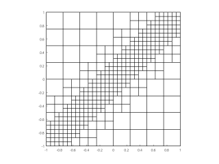
Figure 1: A hierarchical mesh obtained with $M=3$ levels.

In order to define the spline hierarchy, the set of active basis functions $B_{J}^{\ell}$, for each level $\ell$, is selected from ${\cal B}_{\bf d}^{\ell}$ according to the following definition, see also [11, 22].

Definition 1.

The hierarchical B-spline basis ${\cal H}_{\bf d}({\cal G}_{\cal H})$ of degree ${\bf d}$ with respect to the mesh ${\cal G}_{\cal H}$ is defined as

$${\cal H}_{\bf d}({\cal G}_{\cal H}):=\left\{B_{J}^{\ell}\in{\cal B}_{\bf d}^{\ell}\,:\,J\in A_{\bf d}^{\ell},\,\,\ell=0,...,M-1\right\}\,\,,$$

where

$$A_{\bf d}^{\ell}\,:=\,\{J\in\Gamma_{{\bf d},{\bf h}_{\ell}}\,:\,\mathop{\mathrm{supp}}B_{J}^{\ell}\subseteq\Omega^{\ell}\,\,\wedge\,\,\mathop{\mathrm{supp}}B_{J}^{\ell}\not\subseteq\Omega^{\ell+1}\}\,,$$ (14)

is the active set of multi–indices $A_{\bf d}^{\ell}\subseteq\Gamma_{{\bf d},{\bf h}_{\ell}}$ and $\mathop{\mathrm{supp}}B_{J}^{\ell}$ denotes the intersection of the support of $B_{J}^{\ell}$ with $\Omega^{0}$.

The space $S_{\cal H}:=\mathop{\mathrm{span}}{\cal H}_{\bf d}({\cal G}_{\cal H})$ is the hierarchical spline space associated to the mesh ${\cal G}_{\cal H}$. Obviously, $S_{\cal H}$ is a subset of $V^{M-1}\subseteq C^{(d_{1}-1,d_{2}-1)}(\Omega)$. In virtue of the linear independence of hierarchical B–splines, see e.g., [11, 22],

$$\dim(S_{\cal H})\,=\,\sum_{\ell=0}^{M-1}\#A_{\bf d}^{\ell}\,\,\leq\dim(V^{M-1}).$$

Note that, the symbol $\ll$ can usually replace the last $\leq$ inequality symbol, since the adaptive spline framework allows to obtain the desired approximation with a strongly reduced number of degrees of freedom. Furthermore we would like to remark that, even if in general it is only $S_{\cal H}\subseteq S_{{\bf d}}({\cal G_{\cal H}})$, where

$$S_{{\bf d}}({\cal G}_{\cal H}):=\left\{f\in C^{(d_{1}-1,d_{2}-1)}(\Omega):f\!\left.\rule{0.0pt}{8.61108pt}\right|_{c}\in{\mathop{{\rm I}\kern-1.99997pt{\rm P}}\nolimits}^{\bf d},\forall c\in{\cal G}^{\ell},\ell=0,\ldots,M-1\right\},$$

under reasonable assumptions on the hierarchical mesh configuration it is possible to obtain that $S_{\cal H}=S_{{\bf d}}({\cal G_{\cal H}})$ [6].

In order to recover the partition of unity property in the hierarchical setting and reduce the support of coarsest basis function, the truncated hierarchical B-spline (THB–spline) basis of $S_{\cal H}$ has been recently introduced [7]. This alternative hierarchical construction relies on the definition of the following truncation operator $\mathop{\mathrm{trunc}}^{\ell+1}:V^{\ell}\rightarrow V^{\ell+1},\ell=0,\ldots,M-2$.

Definition 2.

Let $s(\cdot)=\displaystyle{\sum_{J\in\Gamma_{{\bf d},{\bf h}_{\ell+1}}}}\sigma_{J}^{\ell+1}B_{J}^{\ell+1}(\cdot)\,,$ be the representation in the B–spline basis of $V^{\ell+1}\supset V^{\ell}\,,$ of $s\in V^{\ell}$. The truncation of $s$ with respect to ${\cal B}^{\ell+1}$ and $\Omega^{\ell+1}$ is defined as

$${\mathop{\mathrm{trunc}}}^{\ell+1}s(\cdot)\,:=\,\displaystyle{\sum_{J\in\Gamma_{{\bf d},{\bf h}_{\ell+1}}\,:\,\mathop{\mathrm{supp}}B_{J}^{\ell+1}\,\not\subseteq\,\Omega^{\ell+1}}}\sigma_{J}^{\ell+1}B_{J}^{\ell+1}(\cdot)\,.$$

By also introducing the operator $Trunc^{\ell+1}:V^{\ell}\rightarrow S_{\cal H}\subseteq V^{M-1}$, for $\ell=0,\ldots,M-1,$

$$Trunc^{\ell+1}\,:=\,trunc^{M-1}(trunc^{M-2}(\cdots(trunc^{\ell+1}(s))\cdots))\,,$$

we are ready to define the truncated basis for $S_{\cal H}\,,$ according to the following construction [7].

Definition 3.

The truncated hierarchical B-spline basis ${\cal T}_{{\bf d}}({\cal G}_{\cal H})$ of degree ${\bf d}$ with respect to the mesh ${\cal G}_{\cal H}$ is defined as

$${\cal T}_{{\bf d}}({\cal G}_{\cal H})\,:=\,\left\{T_{J}^{\ell}\,:\,J\in A_{\bf d}^{\ell},\,\,\ell=0,...,M-1\right\}\,,\,\,\text{with}\quad T_{j}^{\ell}\,:=\,Trunc^{\ell+1}(B_{J}^{\ell})\,.$$ (15)

THB–splines have very important properties like linear independence, non–negativity, partition of unity, preservation of coefficients and strong stability [7, 8]. In particular the preservation of coefficients property is of central interest in the context of quasi–interpolation because it ensures that the hierarchical extension of any tensor–product quasi–interpolation operator keeps its polynomial reproduction capability [18]. Figure 2 shows the two successive steps necessary to obtain the truncated basis element $T_{J}^{0}$ for a certain $J\in A_{\bf d}^{0}$ with respect to the hierarchy of domains shown in Figure 1. Note that, if $\sigma_{J}^{\ell}$ denotes the coefficient of a spline $s\in S_{\cal H}$ in the THB spline basis, since only few truncated basis functions do not vanish on a cell $c$ of the hierarchical mesh, we can write,

$$s(x,y)\,=\,\sum_{\ell=0}^{M-1}\sum_{J\in{\cal A}_{\bf d}^{\ell}(c)}\sigma_{J}^{\ell}T_{J}^{\ell}(x,y)\,,\quad\forall(x,y)\in c\,,$$

where

$${\cal A}_{\bf d}^{\ell}(c)\,:=\,\{J\in A_{\bf d}^{\ell}\,\,|\,\,c\subseteq supp(T_{J}^{\ell})\}\,.$$ (16)

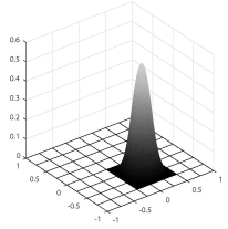
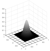
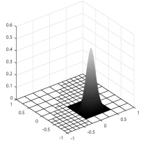
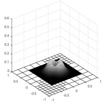
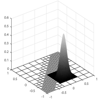
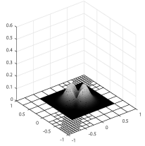
Figure 2: Two examples of elements of the truncated hierarchical B-spline basis. For $(d_{1},d_{2})=(2,2)$, starting from (a) $B_{J}^{0}$, the truncation at level $\ell=1$ gives (c) $trunc^{1}(B_{J}^{0})$, and the further truncation at level $\ell=2$ gives (e) $T_{J}^{2}:=Trunc^{2}(B_{J}^{0}):=trunc^{2}(trunc^{1}(B_{J}^{0}))$. Similarly, (b), (d), (f) represent the successive truncations of a B-spline of bi-degree $(d_{1},d_{2})=(4,4)$.

The truncation of coarsest basis functions with respect to finer basis elements allow to reduce the overlap of supports of basis functions at different hierarchical levels. Nevertheless, in order to have a specific bound for the number of truncated basis functions acting on any cell, suitable hierarchical configurations should be selected.

Definition 4.

A hierarchical mesh ${\cal G}_{\cal H}$ is admissible of class $m$, $1\leq m<M$, if the THB–splines which take non–zero value over any cell $c\in{\cal G}_{\cal H}$ belong to at most $m$ successive levels.

Restricted hierarchies that allow the identification of admissible meshes were considered in [8] for the case $m=2$, and in [3] for a general $m$. If ${\cal G}_{\cal H}$ is an admissible mesh of class $m$ the following remarks can be done,

• if $c\in{\cal G}_{k}\,,$ ${\cal A}_{\bf d}^{\ell}(c)$ can be non empty only if $k_{m}\leq\ell\leq k\,,$ with

  $$k_{m}\,:=\,\max\{0\,,\,k-m+1\}\,;$$ (17)

• $m(d_{1}+1)(d_{2}+1)$ is an upper bound for the number of THB–splines which are non–zero on each cell;

• there exist two positive constants $\gamma_{1}$ and $\gamma_{2}$ depending on the class of admissibility $m$ but not on the other quantities such that, for all $c\in{\cal G}_{\cal H}$ and for each multi–index $J\in{\cal A}_{\bf d}^{\ell}(c)\,,$ it is

  $$\gamma_{1}\mathop{\mathrm{diam}}(c)\leq\mathop{\mathrm{diam}}(\mathop{\mathrm{supp}}T_{J}^{\ell})\leq\gamma_{2}\mathop{\mathrm{diam}}(c)\,.$$

The above properties of hierarchical meshes of class $m$ will be used in the next section to get theoretical proofs of convergence for the considered hierarchical quasi–interpolation scheme.

4 The hierarchical Hermite BS QI scheme

Besides the mentioned advantages, the THB–spline basis of $S_{\cal H}$ has another fundamental advantage with respect to the HB–spline basis because, thanks to its preservation of coefficients property, it allows an easy extension to the hierarchical setting of any quasi–interpolation operator [18]. For example, specifically relating the tensor–product BS QI operator $Q$ defined in (7), we can just define its extension $Q_{\cal H}:C^{1,1}(\Omega_{e})\rightarrow S_{\cal H}$ as follows,

$$Q_{\cal H}(f)(x,y)\,:=\,\sum_{\ell=0}^{M-1}\sum_{J\in A_{{\bf d},{\bf h}_{\ell}}}\lambda_{J}^{\ell}(f)\,T_{J}^{\ell}(x,y)\,,$$ (18)

with $T_{J}^{\ell},\,J\in A_{{\bf d},{\bf h}_{\ell}}\,,\ell=0,\ldots,M-1,$ denoting the truncated basis introduced in (15) and with the functional $\lambda_{J}^{\ell}(f)$ defined as in (10), just replacing $h_{x}$ and $h_{y}$ respectively with $h_{x,\ell}$ and $h_{y,\ell}\,.$ Actually in [18] it has been proved that this definition is reasonable because it ensures the following implication,

$$Q(p)\,=\,p\,,\,\,\forall p\in{\mathop{{\rm I}\kern-1.99997pt{\rm P}}\nolimits}^{\bf d}\quad\Rightarrow\quad Q_{\cal H}(p)=p\,,\,\,\forall p\in{\mathop{{\rm I}\kern-1.99997pt{\rm P}}\nolimits}^{\bf d}\,.$$ (19)

We start with a preliminary lemma.

Lemma 2.

If the hierarchical mesh ${\cal G}_{\cal H}$ is admissible of class $m\,,$ then for any cell $c\in{\cal G}^{k},k=0,\ldots,M-1,$ and for any function $f\in C^{(1,1)}(\Omega_{e}),$ it is

$$\begin{array}[]{ll}\|Q_{\cal H}(f)\|_{c}\,\leq&\kappa_{0,0}\|f\|_{C}+\,2^{m-1}\,h_{x,k}\,\kappa_{1,0}\|f^{(1,0)}\|_{C}+\cr&2^{m-1}\,h_{y,k}\,\kappa_{0,1}\|f^{(0,1)}\|_{C}+\,4^{m-1}h_{x,k}h_{y,k}\kappa_{1,1}\|f^{(1,1)}\|_{C}\,,\cr\end{array}$$

where the positive constants $\kappa_{r,s},r,s=0,1$ are those introduced in Lemma 1 and

$$C\,:=\,\bigcup_{\ell=k_{m}}^{k}\,\bigcup_{J\in{\cal A}_{\bf d}^{\ell}(c)}(\Lambda_{J}^{\ell}\cup c)\,.$$ (20)

Proof : Let $c\in{\cal G}^{k}$. Considering the assumption on ${\cal G}_{\cal H},$ the restriction of $Q_{\cal H}(f)$ to the cell $c$ can be written as follows,

$$Q_{\cal H}(f)_{|c}\,=\,\sum_{\ell=k_{m}}^{k}\sum_{J\in{\cal A}_{\bf d}^{\ell}(c)}\lambda_{J}^{\ell}(f)\,T_{J}^{\ell}\,,$$

with ${\cal A}_{\bf d}^{\ell}(c)$ defined as in (16) and where, for brevity, we have used the integer $k_{m}$ introduced in (17). This expression implies that $Q_{\cal H}(f)_{|c}$ depends on $f_{|C}\,$ where $C\supset c$ is defined as in (20). Now, using the triangular inequality and considering that the THB spline basis is a nonnegative partition of unity, it can be derived that

$$|Q_{\cal H}(f)(x,y)|\,\leq\,\max_{k_{m}\leq\ell\leq k}\,\max_{J\in{\cal A}_{\bf d}^{\ell}(c)}|\lambda_{J}^{\ell}(f)|\,,\quad\forall(x,y)\in c\,.$$ (21)

Thus the statement of the lemma is obtained by considering the functional upper bound proved in Lemma 1 and further uniformly upper bounding each $|\lambda_{J}^{\ell}(f)|$ in (21) by replacing in (12) the function norm $\|\cdot\|_{\Lambda_{J}^{\ell}}$ with $\|\cdot\|_{C}$.  

The following remark outlines the relation which can be established between the size of $C$ and that of $c,$ under the assumed hypothesis on the hierarchical mesh.

Remark 2.

Let $R$ denote the smallest rectangle with edges aligned with the $x$ and $y$ axes containing the convex hull of $C,$ with $C$ defined in (20). Further, let us denote with $H_{x}(C)$ and $H_{y}(C)$ its $x$ and $y$ sizes, also called in the following the $x$ and $y$ diameters of $C\,.$ Then if ${\cal G}_{\cal H}$ is admissible of class $m\,,$ there exist two positive constants $w_{i}>1,i=1,2$ depending only on ${\bf d}$ and on $m$ such that for any cell $c\in{\cal G}^{k},k=0,\ldots,M-1,$ it is

$$H_{x}(C)\leq\,w_{1}h_{x,k}\,,\quad H_{y}(C)\,\leq\,w_{2}h_{y,k}\,.$$ (22)

Actually it can be verified that we can assume

$$w_{i}\,:=\,2^{m-1}\,(d_{i}-1)\,,\quad i=1,2\,.$$ (23)

Then, by using the intermediate result proved in Lemma 2 and the inequality in (22), we are ready to prove the following main result concerning the local approximation power of $Q_{\cal H}(f)\in S_{\cal H}\,.$

Theorem 1.

Let ${\cal G}_{\cal H}$ be admissible of class $m.$ Then there exist three positive constants $v_{i}\,,i=1,2,3$ such that $\forall f\in C^{(d_{1}+1,d_{2}+1)}(\Omega)$ and $\forall c\in{\cal G}^{k},k=0,\ldots,M-1,$ it is,

$$\begin{array}[]{ll}\|f-Q_{\cal H}(f)\|_{c}\,\leq&v_{1}\,\|f^{(d_{1}+1,0)}\|_{C}\,h_{x,k}^{d_{1}+1}+v_{2}\,\|f^{(0,d_{2}+1)}\|_{C}\,h_{y,k}^{d_{2}+1}+\cr&v_{3}\,\|f^{(d_{1}+1,d_{2}+1)}\|_{C}\,h_{x,k}^{d_{1}+1}h_{y,k}^{d_{2}+1}\,,\cr\end{array}$$ (24)

where $C$ is defined in (20).

Proof : Considering that (19) ensures that $Q_{\cal H}(p)=p,\,\,\forall p\in{\mathop{{\rm I}\kern-1.99997pt{\rm P}}\nolimits}^{\bf d},$ then the triangular inequality implies that, $\forall c\in{\cal G}^{k}\,,$ it is

$$\|f-Q_{\cal H}(f)\|_{c}\,\leq\,\|f-p\|_{c}\,+\,\|Q_{\cal H}(p-f)\|_{c}\,,\quad\forall p\in{\mathop{{\rm I}\kern-1.99997pt{\rm P}}\nolimits}^{\bf d}\,.$$

On the other hand, considering that $c\subset C$ with $C$ defined in (20), Lemma 2 implies that

$$\begin{array}[]{ll}\|f-Q_{\cal H}(f)\|_{c}\leq&(1+\kappa_{0,0})\|p-f\|_{C}+\cr&2^{m-1}\,h_{x,k}\,\kappa_{1,0}\|p^{(1,0)}-f^{(1,0)}\|_{C}+\cr&2^{m-1}\,h_{y,k}\,\kappa_{0,1}\|p^{(0,1)}-f^{(0,1)}\|_{C}+\cr&4^{m-1}h_{x,k}h_{y,k}\kappa_{1,1}\|p^{(1,1)}-f^{(1,1)}\|_{C}\,.\cr\end{array}$$

Choosing $p\in{\mathop{{\rm I}\kern-1.99997pt{\rm P}}\nolimits}^{\bf d}$ as the Taylor expansion of $f$ in ${\mathop{{\rm I}\kern-1.99997pt{\rm P}}\nolimits}^{\bf d}$ at some point in $c\,,$ it is

$$\begin{array}[]{ll}\|p^{(r,s)}-f^{(r,s)}\|_{C}\,\leq&\|f^{(d_{1}+1,0)}\|_{C}\,H_{x}(C)^{d_{1}+1-r}+\|f^{(0,d_{2}+1)}\|_{C}\,H_{y}(C)^{d_{2}+1-s}+\cr&\|f^{(d_{1}+1,d_{2}+1)}\|_{C}\,H_{x}(C)^{d_{1}+1-r}H_{y}(C)^{d_{2}+1-s}\,,\,\,r,s=0,1\,,\cr\end{array}$$

where $H_{x}(C)$ and $H_{y}(C)$ denote the $x$ and $y$ diameters of $C$ introduced in Remark 2. Then the thesis is proved by using the inequality given in (22) and by defining $v_{i},i=1,2,3$ as follows,

$$v_{1}\,:=\,K\,w_{1}^{d_{1}+1}\,,\quad v_{2}\,:=\,K\,w_{2}^{d_{2}+1}\,,\quad v_{3}\,:=\,K\,w_{1}^{d_{1}+1}\,w_{2}^{d_{2}+1}\,,$$

with $K\,:=\,1+\kappa_{0,0}+(\kappa_{1,0}+\kappa_{0,1}+\kappa_{1,1})\gamma\,,$ where $\gamma:=2^{m-1}\max\{1\,,h_{x,0}\,,\,h_{y,0}\}$ and where the constants $w_{i},i=1,2\,,$ are those defined in (23).  

Remark 3.

The statement of Theorem 1 first of all says that $Q_{\cal H}$ mantains on a cell $c\in{\cal G}^{k}$ the maximal approximation order of $Q:C^{(1,1)}(\Omega)\rightarrow V^{k}\,.$ Furthermore, in order to guarantee that $Q_{\cal H}$ in $S_{\cal H}$ provides the same approximation quality of $Q$ in $V^{M-1},$ it also suggests to use larger cells where $f^{(d_{1}+1,0)}$ and $f^{(0,d_{2}+1)}$ are almost zero and finer elsewhere.

5 Numerical results

In this section we discuss the numerical behaviour of the hierarchical BS QI operator $Q_{\cal H}$. The test functions $f(x,y)$ considered in the examples are

$$f_{1}(x,y)=\frac{\tanh(9y-9x)+1}{9},\qquad(x,y)\in[-1,1]^{2},$$

$$f_{2}(x,y)=\frac{2}{3\exp((10x-3)^{2}+(10y+4)^{2})},\qquad(x,y)\in[-1,1]^{2},$$

see Figure 3.

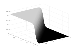
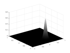
Figure 3: The test functions $f_{1}$ (left) and $f_{2}$ (right).

We compare the performances of $Q_{\cal H}$ with the hierarchical QI considered in the numerical examples in [18]. More precisely, the tensor–product version of this QI [12], here denoted by $\hat{Q}$, is the following,

$$\hat{Q}(f)(x,y):=\sum_{J\in\Gamma_{{\bf d},{\bf h}}}\hat{\lambda}_{J}(f)\,B_{J}^{({\bf d},{\bf h})}(x,y)\,,$$

where each $\hat{\lambda}_{J}(f)$, $J=(j,i)$, is obtained as the component $\sigma_{J}$ of the solution of the linear system

$$\sum_{K:supp(B_{K}^{({\bf d},{\bf h})})\cap\Theta_{J}\neq\emptyset}\sigma_{K}B_{K}^{({\bf d},{\bf h})}({\bf x}^{r_{1},r_{2}}_{J})=f({\bf x}^{r_{1},r_{2}}_{J}),\quad r_{1}=0,...,d_{1},\quad r_{2}=0,...,d_{2},$$

with

$$\Theta_{J}:=(x_{i+\lfloor d_{1}/2\rfloor},x_{i+\lfloor d_{1}/2\rfloor}+1)\times(y_{j+\lfloor d_{2}/2\rfloor},y_{j+\lfloor d_{2}/2\rfloor+1}),$$

$${\bf x}^{r_{1},r_{2}}_{J}:=(x_{i+\lfloor d_{1}/2\rfloor}+\frac{r_{1}h_{x}}{d_{1}},y_{j+\lfloor d_{2}/2\rfloor}+\frac{r_{2}h_{y}}{d_{2}}).$$

The hierarchical extension $\hat{Q}_{\cal H}$ is obtained from $\hat{Q}$ as done for defining $Q_{\cal H}$ from $Q$ in (18). Essentially, the differences between $Q_{\cal H}$ and $\hat{Q}_{\cal H}$ lie in the type of data they use (function and derivative values for $Q_{\cal H}$ and only function values for $\hat{Q}_{\cal H}$), and in the number and kind of data locations.

In all the tests, we considered sequences of nested hierarchical meshes on the domain $[-1,1]^{2}$ up to $5$ levels ($M=5$), obtained by suitably refining a uniform $8\times 8$ mesh. For all tests, the tables reporting the results obtained by applying the hierarchical QIs show the number of levels $M$, the size of the mesh $h_{M-1}:=h_{x,M-1}=h_{y,M-1}$ at the finest level, the dimension of the spline spaces and the infinity norm $\|\cdot\|_{\Omega}$ of the errors

$$e:=f-Q(f),\quad e_{\cal H}:=f-Q_{\cal H}(f),\quad\hat{e}:=f-\hat{Q}(f),\quad\hat{e}_{\cal H}:=f-Q_{\cal H}(f)\,.$$

Note that the infinity norm $\|\cdot\|_{\Omega}$ of a function has always been numerically approximated by computing the maximum of its absolute value on a $301\times 301$ uniform grid of $\Omega\,.$ Moreover, in order to have a complete understanding of the behaviour of the QIs, we also report the infinity norms of the errors with respect to the derivatives $f_{x}$, $f_{y}$ and $f_{xy}$.

The employed hierarchical meshes are obtained by applying an automatic refinement strategy. Let $F_{\cal H}$ be the hierarchical extension, based on the mesh ${\cal G_{H}}$ with $M$ levels, of a tensor-product QI operator $F$, and let $P\subset\Omega$ be a set of points where the values of the approximated function $f$ (and of its derivatives, if the computation of $F$ requires them, like in the case of $Q$) are available. Let us define, for each cell $c\in{\cal G_{H}}$,

$$\delta(F_{\cal H};c):=\max_{(x,y)\in P\cap c}|F_{\cal H}(x,y)-f(x,y)|.$$

Then, the hierarchical mesh is generated by using the following algorithm.

• Start from a tensor-product mesh, which corresponds to a hierarchical mesh ${\cal G_{H}}$ with $1$ level ($M=1$), choose the maximum number of levels $K$ ($K=5$ in our tests) and the tolerance $\epsilon$;

• evaluate the corresponding $F_{\cal H}$ at the points $(x,y)\in P$;

• while $\delta(F_{\cal H};c)\leq\epsilon$ is not satisfied for all the cells $c\in{\cal G_{H}}$, or $M$ is not greater than $K$, repeat the following steps:

  • mark the cells which do not satisfy $\delta(F_{\cal H};c)\leq\epsilon$;

  • for each marked cell, additionally mark the (at most) $8$ adjacent cells too;

  • obtain the new mesh ${\cal G_{H}}$ with $M+1$ levels by a dyadic split of the marked cells, and increase $M$ by $1$;

  • evaluate the corresponding $F_{\cal H}$ at the points $(x,y)\in P$.

Now, in our case the main goal is to construct a hierarchical QI operator $F_{\cal H}$ with approximation performances close to those of its tensor-product version $F$ defined using the required information on the extended lattice $\pi^{e}$ associated with level $K.$ Then we set $P=\pi^{e}\cap\Omega$ and

$$\epsilon=1.5\max_{(x,y)\in P}|F(x,y)-f(x,y)|,$$

which, roughly speaking, corresponds to requiring that the use of the hierarchical QI provides a maximum error at most 50% larger than the one provided by the tensor-product version of the QI. As in our experiments $K=5$ and at the first level we use a $8\times 8$ mesh, $P$ is composed of the vertices of a uniform $128\times 128$ grid in $\Omega.$

Tables 2-3 and 4-5 report the results related to $f_{1}$ obtained with $(d_{1},d_{2})=(2,2),(3,3),(4,4)$ for $Q_{\cal H}$ and for $\hat{Q}_{\cal H}$, respectively.

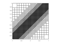
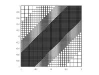
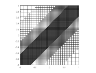
Figure 4: The hierarchical meshes with 5 levels used in the approximation of $f_{1}$ by $Q_{\cal H}$ with (a) $(d_{1},d_{2})=(2,2)$, (b) $(d_{1},d_{2})=(3,3)$ and (c) $(d_{1},d_{2})=(4,4)$.

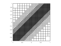
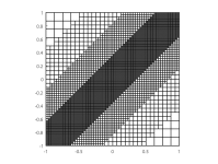
Figure 5: The hierarchical meshes with 5 levels used in the approximation of $f_{1}$ by $\hat{Q}_{\cal H}$ with (a) $(d_{1},d_{2})=(2,2)$, (b) $(d_{1},d_{2})=(3,3)$ and (c) $(d_{1},d_{2})=(4,4)$.

$(d_{1},d_{2})=(2,2)$ $M$ ${h}_{M-1}$ $\dim(V^{M-1}$) $\|e\|_{\Omega}$ $\dim(S_{\cal H})$ $\|e_{\cal H}\|_{\Omega}$ $1$ 1/4 100 3.050e-2 100 3.050e-2 $2$ 1/8 324 9.982e-3 310 9.982e-3 $3$ 1/16 1156 1.526e-3 862 1.526e-3 $4$ 1/32 4356 1.312e-4 2368 1.312e-4 $5$ 1/64 16900 1.250e-5 5902 1.250e-5 $(d_{1},d_{2})=(3,3)$ $M$ ${h}_{M-1}$ $\dim(V^{M-1}$) $\|e\|_{\Omega}$ $\dim(S_{\cal H})$ $\|e_{\cal H}\|_{\Omega}$ $1$ 1/4 121 4.581e-2 121 4.581e-2 $2$ 1/8 361 8.168e-3 361 8.168e-3 $3$ 1/16 1225 5.951e-4 1117 5.951e-4 $4$ 1/32 4489 2.414e-5 3139 2.414e-5 $5$ 1/64 17161 1.115e-6 7873 1.115e-6 $(d_{1},d_{2})=(4,4)$ $M$ ${h}_{M-1}$ $\dim(V^{M-1}$) $\|e\|_{\Omega}$ $\dim(S_{\cal H})$ $\|e_{\cal H}\|_{\Omega}$ $1$ 1/4 144 6.842e-2 144 6.842e-2 $2$ 1/8 400 1.034e-2 400 1.034e-2 $3$ 1/16 1296 3.980e-4 1172 3.980e-4 $4$ 1/32 4624 8.828e-6 3056 8.828e-6 $5$ 1/64 17424 1.512e-7 6756 1.512e-7

Table 2: Numerical results for $Q_{\cal H}$ tested on $f_{1}$ and compared with $Q$.

$(d_{1},d_{2})=(2,2)$ $M$ $\|e_{x}\|_{\Omega}$ $\|e_{y}\|_{\Omega}$ $\|e_{xy}\|_{\Omega}$ $\|(e_{\cal H})_{x}\|_{\Omega}$ $\|(e_{\cal H})_{y}\|_{\Omega}$ $\|(e_{\cal H})_{xy}\|_{\Omega}$ $1$ 4.933e-1 4.933e-1 6.185e-0 4.933e-1 4.933e-1 6.185e-0 $2$ 2.218e-1 2.218e-1 4.133e-0 2.218e-1 2.218e-1 4.133e-0 $3$ 5.266e-2 5.266e-2 1.537e-0 5.266e-2 5.266e-2 1.537e-0 $4$ 1.017e-2 1.017e-2 3.019e-1 1.017e-2 1.017e-2 3.019e-1 $5$ 3.088e-3 3.088e-3 1.113e-1 3.088e-3 3.088e-3 1.113e-1 $(d_{1},d_{2})=(3,3)$ $M$ $\|e_{x}\|_{\Omega}$ $\|e_{y}\|_{\Omega}$ $\|e_{xy}\|_{\Omega}$ $\|(e_{\cal H})_{x}\|_{\Omega}$ $\|(e_{\cal H})_{y}\|_{\Omega}$ $\|(e_{\cal H})_{xy}\|_{\Omega}$ $1$ 6.339e-1 6.339e-1 6.600e-0 6.339e-1 6.339e-1 6.600e-0 $2$ 1.812e-1 1.812e-1 3.741e-0 1.812e-1 1.812e-1 3.741e-0 $3$ 1.835e-2 1.835e-2 7.533e-1 1.835e-2 1.835e-2 7.533e-1 $4$ 1.263e-3 1.263e-3 7.065e-2 1.263e-3 1.263e-3 7.065e-2 $5$ 9.971e-5 9.971e-5 6.179e-3 9.972e-5 9.972e-5 6.179e-3 $(d_{1},d_{2})=(4,4)$ $M$ $\|e_{x}\|_{\Omega}$ $\|e_{y}\|_{\Omega}$ $\|e_{xy}\|_{\Omega}$ $\|(e_{\cal H})_{x}\|_{\Omega}$ $\|(e_{\cal H})_{y}\|_{\Omega}$ $\|(e_{\cal H})_{xy}\|_{\Omega}$ $1$ 8.318e-1 8.318e-1 7.401e-0 8.318e-1 8.318e-1 7.401e-0 $2$ 2.212e-1 2.212e-1 4.012e-0 2.212e-1 2.212e-1 4.012e-0 $3$ 1.457e-2 1.457e-2 5.285e-1 1.457e-2 1.457e-2 5.285e-1 $4$ 4.846e-4 4.846e-4 2.389e-2 4.846e-4 4.846e-4 2.389e-2 $5$ 1.401e-5 1.401e-5 6.941e-4 1.401e-5 1.401e-5 6.941e-4

Table 3: Errors with respect to the derivatives for $Q_{\cal H}$ tested on $f_{1}$ and compared with $Q$.

$(d_{1},d_{2})=(2,2)$ $M$ ${h}_{M-1}$ $\dim(V^{M-1}$) $\|\hat{e}\|_{\Omega}$ $\dim(S_{\cal H})$ $\|\hat{e}_{\cal H}\|_{\Omega}$ $1$ 1/4 100 4.165e-2 100 4.165e-2 $2$ 1/8 324 1.007e-2 310 1.007e-2 $3$ 1/16 1156 1.292e-3 862 1.292e-3 $4$ 1/32 4356 1.160e-4 2368 1.160e-4 $5$ 1/64 16900 1.109e-5 5902 1.109e-5 $(d_{1},d_{2})=(3,3)$ $M$ ${h}_{M-1}$ $\dim(V^{M-1}$) $\|\hat{e}\|_{\Omega}$ $\dim(S_{\cal H})$ $\|\hat{e}_{\cal H}\|_{\Omega}$ $1$ 1/4 121 7.646e-2 121 7.646e-2 $2$ 1/8 361 1.290e-2 361 1.290e-2 $3$ 1/16 1225 4.584e-4 1075 4.584e-4 $4$ 1/32 4489 1.123e-5 2971 1.123e-5 $5$ 1/64 17161 9.183e-7 7393 9.183e-7 $(d_{1},d_{2})=(4,4)$ $M$ ${h}_{M-1}$ $\dim(V^{M-1}$) $\|\hat{e}\|_{\Omega}$ $\dim(S_{\cal H})$ $\|\hat{e}_{\cal H}\|_{\Omega}$ $1$ 1/4 144 1.015e-1 144 1.015e-1 $2$ 1/8 400 2.945e-2 400 2.945e-2 $3$ 1/16 1296 4.799e-4 1172 4.799e-4 $4$ 1/32 4624 1.061e-5 3186 1.061e-5 $5$ 1/64 17424 1.980e-7 6886 1.980e-7

Table 4: Numerical results for $\hat{Q}_{\cal H}$ tested on $f_{1}$ and compared with $\hat{Q}$.

$(d_{1},d_{2})=(2,2)$ $M$ $\|\hat{e}_{x}\|_{\Omega}$ $\|\hat{e}_{y}\|_{\Omega}$ $\|\hat{e}_{xy}\|_{\Omega}$ $\|(\hat{e}_{\cal H})_{x}\|_{\Omega}$ $\|(\hat{e}_{\cal H})_{y}\|_{\Omega}$ $\|(\hat{e}_{\cal H})_{xy}\|_{\Omega}$ $1$ 5.988e-1 5.988e-1 6.451e-0 5.988e-1 5.988e-1 6.451e-0 $2$ 2.229e-1 2.229e-1 4.127e-0 2.229e-1 2.229e-1 4.127e-0 $3$ 4.645e-2 4.645e-2 1.425e-0 4.645e-2 4.645e-2 1.425e-0 $4$ 1.101e-2 1.101e-2 3.193e-1 1.101e-2 1.101e-2 3.193e-1 $5$ 3.152e-3 3.152e-3 1.150e-1 3.152e-3 3.152e-3 1.150e-1 $(d_{1},d_{2})=(3,3)$ $M$ $\|\hat{e}_{x}\|_{\Omega}$ $\|\hat{e}_{y}\|_{\Omega}$ $\|\hat{e}_{xy}\|_{\Omega}$ $\|(\hat{e}_{\cal H})_{x}\|_{\Omega}$ $\|(\hat{e}_{\cal H})_{y}\|_{\Omega}$ $\|(\hat{e}_{\cal H})_{xy}\|_{\Omega}$ $1$ 8.666e-1 8.666e-1 7.183e-0 8.666e-1 8.666e-1 7.183e-0 $2$ 2.525e-1 2.525e-1 4.271e-0 2.525e-1 2.525e-1 4.271e-0 $3$ 1.709e-2 1.709e-2 6.800e-1 1.709e-2 1.709e-2 6.800e-1 $4$ 9.541e-4 9.541e-4 6.068e-2 9.541e-4 9.541e-4 6.068e-2 $5$ 1.001e-4 1.001e-4 6.504e-3 1.001e-4 1.001e-4 6.504e-3 $(d_{1},d_{2})=(4,4)$ $M$ $\|\hat{e}_{x}\|_{\Omega}$ $\|\hat{e}_{y}\|_{\Omega}$ $\|\hat{e}_{xy}\|_{\Omega}$ $\|(\hat{e}_{\cal H})_{x}\|_{\Omega}$ $\|(\hat{e}_{\cal H})_{y}\|_{\Omega}$ $\|(\hat{e}_{\cal H})_{xy}\|_{\Omega}$ $1$ 5.247e-1 5.247e-1 5.096e-0 5.247e-1 5.247e-1 5.096e-0 $2$ 4.704e-1 4.704e-1 5.823e-0 4.704e-1 4.704e-1 5.823e-0 $3$ 1.687e-2 1.687e-2 5.774e-1 1.687e-2 1.687e-2 5.774e-1 $4$ 5.538e-4 5.538e-4 2.597e-2 5.538e-4 5.538e-4 2.597e-2 $5$ 1.623e-5 1.623e-5 7.786e-4 1.623e-5 1.623e-5 7.786e-4

Table 5: Errors with respect to the derivatives for $\hat{Q}_{\cal H}$ tested on $f_{1}$ and compared with $\hat{Q}$.

We further compared $Q_{\cal H}$ and $\hat{Q}_{\cal H}$ by examining the functional evaluations needed in the two cases: as shown in Table 6, while for $(d_{1},d_{2})=(2,2)$ the number of required evaluations is smaller for $\hat{Q}_{\cal H}$, when $(d_{1},d_{2})=(3,3),(4,4)$ $\hat{Q}_{\cal H}$ requires significantly more evaluations than $Q_{\cal H}$, in spite of using, in some cases, slightly less refined hierarchical meshes (which lead to spline spaces with smaller dimension). Note that for the corresponding tensor–product versions, the number of evaluations is $4(N_{1}+2d_{1}-1)(N_{2}+2d_{2}-1)$ for $Q$ and $(d_{1}(N_{1}+d_{1})+1)(d_{2}(N_{2}+d_{2})+1)$ for $\hat{Q}$, which is the reason behind the increasing difference between the evaluations needed by $Q_{\cal H}$ and $\hat{Q}_{\cal H}$ as $d_{1}$ and $d_{2}$ grow.

Tables 7-8 and 9-10 report, respectively, the results for $Q_{\cal H}$ and for $\hat{Q}_{\cal H}$ applied to $f_{2}$ with $(d_{1},d_{2})=(3,3)$. In this case, we can observe that at the coarsest levels $Q_{\cal H}$ and $\hat{Q}_{\cal H}$ behave differently, with $Q_{\cal H}$ showing a better accuracy. Note that such differences are not related to the hierarchical nature of the QIs, since the same behaviour can be observed in their tensor–product versions (as in the previous case, the choice of the hierarchical meshes allows to obtain essentially the same maximum error as in the tensor–product case).

$(d_{1},d_{2})=(2,2)$ $M$ 1 2 3 4 5 $Q$ 484 1444 4900 17956 68644 $\hat{Q}$ 441 1369 4761 17689 68121 $Q_{\cal H}$ 484 1404 3756 10052 24716 $\hat{Q}_{\cal H}$ 441 1299 3501 9471 23433 $(d_{1},d_{2})=(3,3)$ $M$ 1 2 3 4 5 $Q$ 676 1764 5476 19044 70756 $\hat{Q}$ 1156 3364 11236 40804 155236 $Q_{\cal H}$ 676 1764 5076 13708 33700 $\hat{Q}_{\cal H}$ 1156 3364 9732 26498 65446 $(d_{1},d_{2})=(4,4)$ $M$ 1 2 3 4 5 $Q$ 900 2116 6084 20166 72900 $\hat{Q}$ 2401 6561 21025 74529 279841 $Q_{\cal H}$ 900 2116 5684 14084 30516 $\hat{Q}_{\cal H}$ 2401 6561 18641 49825 106065

Table 6: Number of functional evaluations needed by $Q$, $\hat{Q}$, $Q_{\cal H}$ and $\hat{Q}_{\cal H}$ in the test on $f_{1}$.

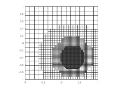
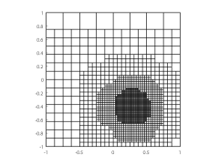
Figure 6: The hierarchical meshes with 5 levels used to approximate $f_{2}$ by $Q_{\cal H}$ (right) and by $\hat{Q}_{\cal H}$ (left) with $(d_{1},d_{2})=(3,3)$.

$M$ ${h}_{M-1}$ $\dim(V^{M-1}$) $\|e\|_{\Omega}$ $\dim(S_{\cal H})$ $\|e_{\cal H}\|_{\Omega}$ $1$ 1/4 121 5.763e-1 121 5.763e-1 $2$ 1/8 361 1.974e-1 361 1.974e-1 $3$ 1/16 1225 1.662e-2 787 1.662e-2 $4$ 1/32 4489 6.559e-4 1471 6.559e-4 $5$ 1/64 17161 2.760e-5 2440 2.760e-5

Table 7: Numerical results for $Q_{\cal H}$ tested on $f_{2}$ with $(d_{1},d_{2})=(3,3)$ and compared with $Q$.

$M$ $\|e_{x}\|_{\Omega}$ $\|e_{y}\|_{\Omega}$ $\|e_{xy}\|_{\Omega}$ $\|(e_{\cal H})_{x}\|_{\Omega}$ $\|(e_{\cal H})_{y}\|_{\Omega}$ $\|(e_{\cal H})_{xy}\|_{\Omega}$ $1$ 5.732e-0 6.403e-0 5.385e+1 5.732e-0 6.403e-0 5.385e+1 $2$ 3.504e-0 2.585e-0 3.181e+1 3.504e-0 2.585e-0 3.181e+1 $3$ 4.127e-1 4.067e-1 4.762e-0 4.127e-1 4.067e-1 4.762e-0 $4$ 2.581e-2 2.620e-2 2.736e-1 2.581e-2 2.620e-2 2.736e-1 $5$ 2.531e-3 2.537e-3 2.414e-2 2.531e-3 2.537e-3 2.414e-2

Table 8: Errors with respect to the derivatives for $Q_{\cal H}$ tested on $f_{2}$ with $(d_{1},d_{2})=(3,3)$ and compared with $Q$.

$M$ ${h}_{M-1}$ $\dim(V^{M-1}$) $\|\hat{e}\|_{\Omega}$ $\dim(S_{\cal H})$ $\|\hat{e}_{\cal H}\|_{\Omega}$ $1$ 1/4 121 3.087e-0 121 3.087e-0 $2$ 1/8 361 2.285e-1 310 2.285e-1 $3$ 1/16 1225 1.311e-2 667 1.311e-2 $4$ 1/32 4489 6.365e-4 1210 6.365e-4 $5$ 1/64 17161 3.154e-5 1846 3.154e-5

Table 9: Numerical results for $\hat{Q}_{\cal H}$ tested on $f_{2}$ with $(d_{1},d_{2})=(3,3)$ and compared with $\hat{Q}$.

$M$ $\|\hat{e}_{x}\|_{\Omega}$ $\|\hat{e}_{y}\|_{\Omega}$ $\|\hat{e}_{xy}\|_{\Omega}$ $\|(\hat{e}_{\cal H})_{x}\|_{\Omega}$ $\|(\hat{e}_{\cal H})_{y}\|_{\Omega}$ $\|(\hat{e}_{\cal H})_{xy}\|_{\Omega}$ $1$ 1.203e+1 1.300e+1 7.423e+1 1.203e+1 1.300e+1 7.423e+1 $2$ 4.189e-0 2.944e-0 3.652e+1 4.189e-0 2.944e-0 3.652e+1 $3$ 4.064e-1 4.744e-1 5.057e-0 4.064e-1 4.744e-1 5.057e-0 $4$ 3.313e-2 3.374e-2 3.442e-1 3.313e-2 3.374e-2 3.442e-1 $5$ 2.961e-3 2.714e-3 2.918e-2 2.961e-3 2.714e-3 5.931e-2

Table 10: Errors with respect to the derivatives for $\hat{Q}_{\cal H}$ tested on $f_{2}$ with $(d_{1},d_{2})=(3,3)$ and compared with $\hat{Q}$.

Finally, we present two test where we approximated $f_{1}$ and $f_{2}$ with a modified version of the operator $Q_{\cal H}$, denoted by $Q^{a}_{\cal H}$, which does not require the derivative values. In this case the computation of each functional coefficient $\lambda_{J}^{\ell}(f)$ defining in (18) the hierarchical quasi–interpolant is done by replacing the derivative values with their suitable finite-differences approximations which are locally defined just in terms of function values at the vertices of the uniform grid of level $\ell,\,G^{\ell}\,.$ The only constraint needed to maintain the approximation order of the original QI is to use finite differences approximations of order $(k_{1},k_{2})$ such that $k_{1}\geq d_{1}$ and $k_{2}\geq d_{2}$ (see [16] for some details on these approximations and [9, 10] for their extensions to the tensor–product case). In our tests with $(d_{1},d_{2})=(3,3)$ we used a finite-difference scheme of order $(k_{1},k_{2})=(3,3)$ and, in order to simplify the implementation, we have used the same formulas for the inner points in the whole domains, so taking the necessary gridded function values from a suitably further enlarged domain. The results obtained show that the performances of $Q^{a}_{\cal H}$ are essentially the same as the ones of $Q_{\cal H}$ – see Tables 11-14, which also report the results obtained with the tensor–product version of $Q^{a}_{\cal H}$, denoted by $Q^{a}$. It is worth noting that, in order to obtain with $Q^{a}_{\cal H}$ essentially the same error as with $Q^{a}$, we had to consider meshes with refined areas larger than the ones used with $Q_{\cal H}$. This is in accordance with Theorem 1, since replacing the derivatives with finite-differences schemes enlarges the support of the functionals $\lambda_{J}^{\ell}$ and, as a consequence, the diameter of the set $C$ defined in (20).

For brevity, in the tables we use the following notation,

$$e^{a}:=f-Q^{a}(f),\qquad e^{a}_{\cal H}:=f-Q^{a}_{\cal H}(f).$$

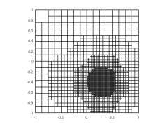
Figure 7: The hierarchical meshes with 5 levels used in the approximation of (a) $f_{1}$ and (b) $f_{2}$ with $Q^{a}_{\cal H}$, $(d_{1},d_{2})=(3,3)$ and $(k_{1},k_{2})=(3,3)$.

$M$ ${h}_{M-1}$ $\dim(V^{M-1}$) $\|e^{a}\|_{\Omega}$ $\dim(S_{\cal H})$ $\|e^{a}_{\cal H}\|_{\Omega}$ $1$ 1/4 121 2.538e-2 121 2.538e-2 $2$ 1/8 361 4.324e-3 361 4.324e-3 $3$ 1/16 1225 4.660e-4 1153 4.660e-4 $4$ 1/32 4489 2.429e-5 3175 2.429e-5 $5$ 1/64 17161 6.323e-7 7597 6.323e-7

Table 11: Numerical results for the modified $Q^{a}_{\cal H}$ (derivatives approximated with order 3 finite-differences scheme) tested on $f_{1}$ with bi-degree $(3,3)$.

$M$ $\|(e_{a})_{x}\|_{\Omega}$ $\|(e_{a})_{y}\|_{\Omega}$ $\|(e_{a})_{xy}\|_{\Omega}$ $\|(e^{a}_{\cal H})_{x}\|_{\Omega}$ $\|(e^{a}_{\cal H})_{y}\|_{\Omega}$ $\|(e^{a}_{\cal H})_{xy}\|_{\Omega}$ $1$ 4.302e-1 4.302e-1 5.983e-0 4.302e-1 4.302e-1 5.983e-0 $2$ 1.172e-1 1.172e-1 3.057e-0 1.172e-1 1.172e-1 3.057e-0 $3$ 1.601e-2 1.601e-2 6.348e-1 1.601e-2 1.601e-2 6.348e-1 $4$ 1.191e-3 1.191e-3 6.229e-2 1.191e-3 1.191e-3 6.229e-2 $5$ 1.052e-4 1.052e-4 6.695e-3 1.052e-4 1.052e-4 6.695e-3

Table 12: Errors with respect to the derivatives for $Q^{a}_{\cal H}$ tested on $f_{1}$ with $(d_{1},d_{2})=(3,3)$ and compared with $Q_{a}$.

$M$ ${h}_{M-1}$ $\dim(V^{M-1}$) $\|e^{a}\|_{\Omega}$ $\dim(S_{\cal H})$ $\|e^{a}_{\cal H}\|_{\Omega}$ $1$ 1/4 121 5.043e-1 121 5.043e-1 $2$ 1/8 361 1.548e-1 352 1.548e-1 $3$ 1/16 1225 2.035e-2 772 2.035e-2 $4$ 1/32 4489 1.869e-3 1417 1.869e-3 $5$ 1/64 17161 8.458e-5 2155 8.458e-5

Table 13: Numerical results for the modified $Q^{a}_{\cal H}$ (derivatives approximated with order 3 finite-differences scheme) tested on $f_{2}$ with bi-degree $(3,3)$.

$M$ $\|(e_{a})_{x}\|_{\Omega}$ $\|(e_{a})_{y}\|_{\Omega}$ $\|(e_{a})_{xy}\|_{\Omega}$ $\|(e^{a}_{\cal H})_{x}\|_{\Omega}$ $\|(e^{a}_{\cal H})_{y}\|_{\Omega}$ $\|(e^{a}_{\cal H})_{xy}\|_{\Omega}$ $1$ 5.448e-0 5.804e-0 4.937e+1 5.448e-0 5.804e-0 4.937e+1 $2$ 2.893e-0 2.405e-0 2.835e+1 2.893e-0 2.405e-0 2.835e+1 $3$ 5.013e-1 5.085e-1 4.613e-0 5.013e-1 5.085e-1 4.613e-0 $4$ 5.468e-2 5.602e-2 5.841e-1 5.468e-2 5.602e-2 5.841e-1 $5$ 4.195e-3 4.124e-3 4.198e-2 4.195e-3 4.124e-3 9.306e-2

Table 14: Errors with respect to the derivatives for $Q^{a}_{\cal H}$ tested on $f_{2}$ with $(d_{1},d_{2})=(3,3)$ and compared with $Q_{a}$.

We note that also for the first and second mixed derivatives the errors produced by the hierarchical approach are essentially equal to those generated by the corresponding tensor–product QIs.

6 Conclusions

The bivariate hierarchical extension of the BS Hermite spline QI scheme has been introduced. The convergence properties of the adaptive construction have been presented together with a detailed analysis of performances and costs, also in comparison with a different hierarchical quasi–interpolation method. For the numerical experiments, we constructed and used an automatic mesh refinement algorithm producing hierarchical meshes which in the considered examples allowed to reach the same accuracy of tensor–product quasi–interpolants but considering hierarchical spline spaces with remarkably lower dimension. Furthermore, it has been verified that a variant of the scheme that does not require information on the derivatives has similar features.

References

- [1] D. Berdinsky, T. Kim, D. Cho, C. Bracco and S. Kiatpanichgij. Bases of T-meshes and the refinement of hierarchical B-splines. Comput. Methods Appl. Mech. Engrg., 283:841–855, 2014.
- [2] C. de Boor and M. G. Fix. Spline approximation by quasi–interpolants. J. Approx. Theory, 8:19–45, 1973.
- [3] A. Buffa and C. Giannelli. Adaptive isogeometric methods with hierarchical splines: error estimator and convergence. Math. Models Methods Appl. Sci., 26: 1–25, 2016.
- [4] C. Dagnino, S. Remogna, and P. Sablonniere. Error bounds on the approximation of functions and partial derivatives by quadratic spline quasi–interpolants on non–uniform criss–cross triangulations of a rectangular domain. J. Comput. Appl. Math., 239:162–178, 2013.
- [5] T. Dokken, T. Lyche, K. F. Pettersen. Polynomial splines over locally refined box–partitions. Comput. Aided Geom. Design, 30:331–356, 2013.
- [6] C. Giannelli and B. Jüttler. Bases and dimensions of bivariate hierarchical tensor–product splines. J. Comput. Appl. Math., 239:162–178, 2013.
- [7] C. Giannelli, B. Jüttler, and H. Speleers. THB–splines: the truncated basis for hierarchical splines. Comput. Aided Geom. Design, 29:485–498, 2012.
- [8] C. Giannelli, B. Jüttler, and H. Speleers. Strongly stable bases for adaptively refined multilevel spline spaces. Adv. Comp. Math., 40:459–490, 2014.
- [9] A. Iurino. BS Hermite Quasi-Interpolation Methods for Curves and Surfaces. PhD thesis, Università di Bari, 2014.
- [10] A. Iurino, F. Mazzia. The C library QIBSH for Hermite Quasi-Interpolation of Curves and Surfaces. Dipartimento di Matematica, Università degli Studi di Bari, report 11/2013, 2013.
- [11] R. Kraft. Adaptive and linearly independent multilevel B–splines. In A. Le Méhauté, C. Rabut, and L. L. Schumaker, editors, Surface Fitting and Multiresolution Methods, pages 209–218. Vanderbilt University Press, Nashville, 1997.
- [12] B. G. Lee, T. Lyche and K. Mørken. Some examples of quasi–interpolants constructed from local spline projectors. In T. Lyche and L. L. Schumaker, editors, Mathematical Methods for Curves and Surfaces: Oslo 2000, pages 243–252. Vanderbilt University Press, Nashville, 2001.
- [13] X. Li, J. Deng, F. Chen. Polynomial splines over general T-meshes. Visual Comput., 26:277–286, 2010.
- [14] T. Lyche and L. L. Schumaker,. Local spline approximation. J. Approx. Theory, 15:294–325, 1975.
- [15] F. Mazzia, A. Sestini. The BS class of Hermite spline quasi–interpolants on nonuniform knot distributions. BIT, 49:611–628, 2009.
- [16] F. Mazzia, A. Sestini. Quadrature formulas descending from BS Hermite spline quasi-interpolation. J. Comput. Appl. Math., 236: 4105–4118, 2012.
- [17] D. Mokriš, B. Jüttler and C. Giannelli. On the completeness of hierarchical tensor–product B-splines. J. Comput. Appl. Math., 271: 53–70, 2014.
- [18] H. Speleers, C. Manni. Effortless quasi-interpolation in hierarchical spaces. Numer. Math., 132: 155–184, 2016.
- [19] P. Sablonniere. Recent progress on univariate and multivariate polynomial and spline quasi–interpolants, trends and applications in constructive approximation. In M. G. de Bruin, D. H. Mache and J. Szabados, editors, International Series of Numerical Mathematics, volume 151, pages 229–245, 2005.
- [20] T. W. Sederberg, D. L. Cardon, G. T. Finnigan, N. S. North, J. Zheng, T. Lyche. T-spline Simplification and Local Refinement. ACM Trans. Graphics, 23:276–283, 2004.
- [21] L. L. Schumaker, L. Wang. Approximation power of polynomial splines on T–meshes. Comput. Aided Geom. Design, 29:599–612, 2012.
- [22] A. V. Vuong, C. Giannelli, B. Jüttler, B. Simeon. A hierarchical approach to adaptive local refinement in isogeometric analysis. Comput. Methods Appl. Mech. Engrg., 200:3554-3567, 2011.