B fields in OB stars (BOB): Detection of a magnetic field in the
He-strong star CPD $-$57^∘ 3509^,

Abstract

Aims. We report the detection of a magnetic field in the helium-strong star CPD $-57^{\circ}$ 3509 (B2 IV), a member of the Galactic open cluster NGC 3293, and characterise the star’s atmospheric and fundamental parameters.

Methods. Spectropolarimetric observations with FORS2 and HARPSpol are analysed using two independent approaches to quantify the magnetic field strength. A high-S/N FLAMES/GIRAFFE spectrum is analysed using a hybrid non-LTE model atmosphere technique. Comparison with stellar evolution models constrains the fundamental parameters of the star.

Results. We obtain a firm detection of a surface averaged longitudinal magnetic field with a maximum amplitude of about 1 kG. Assuming a dipolar configuration of the magnetic field, this implies a dipolar field strength larger than 3.3 kG. Moreover, the large amplitude and fast variation (within about 1 day) of the longitudinal magnetic field implies that CPD $-57^{\circ}$ 3509 is spinning very fast despite its apparently slow projected rotational velocity. The star should be able to support a centrifugal magnetosphere, yet the spectrum shows no sign of magnetically confined material; in particular, emission in H$\alpha$ is not observed. Apparently, the wind is either not strong enough for enough material to accumulate in the magnetosphere to become observable or, alternatively, some leakage process leads to loss of material from the magnetosphere. The quantitative spectroscopic analysis of the star yields an effective temperature and a logarithmic surface gravity of 23 750$\pm$250 K and 4.05$\pm$0.10, respectively, and a surface helium fraction of 0.28$\pm$0.02 by number. The surface abundances of C, N, O, Ne, S, and Ar are compatible with the cosmic abundance standard, whereas Mg, Al, Si, and Fe are depleted by about a factor of 2. This abundance pattern can be understood as the consequence of a fractionated stellar wind. CPD $-57^{\circ}$ 3509 is one of the most evolved He-strong stars known with an independent age constraint due to its cluster membership.

1 Introduction

Helium-strong stars (often also called He-rich stars) constitute the hottest and most massive chemically peculiar (CP) stars of the upper main sequence (e.g. Smith, 1996). They typically populate the temperature domain of $\sim$20 000 – 25 000 K, coinciding with a spectral type around B2. Their helium lines are anomalously strong for their colours, implying abundance ratios of He/H $\sim$ 0.5 by number, while their hydrogen lines are essentially normal, and the metal lines show no outstanding anomalies (Walborn, 1983). The prototype He-strong star discussed in the literature is $σ$ Ori E (Greenstein & Wallerstein, 1958), and only several tens of members of this rare class of stars are known to date. Few systematic investigations of the properties of small samples of He-strong stars are found in the literature (Zboril et al., 1997; Zboril & North, 1999; Leone et al., 1997; Cidale et al., 2007; Zboril, 2011).

Figure 1: Comparison of the FLAMES/GIRAFFE (black line) and the combined HARPSpol Stokes $I$ spectrum (grey line) of CPD $-57^{\circ}$ 3509 for several strategic lines, as indicated. The observed spectra were cross-correlated with the model spectrum computed for our final set of parameters to determine the barycentric radial velocity, and shifted to the laboratory frame for the comparison. See the text for further discussion.

The He-strong stars include some of the strongest magnetic fields detected in non-degenerate stars (e.g. Borra & Landstreet, 1979; Bohlender et al., 1987; Hubrig et al., 2015b). These magnetic fields suppress atmospheric turbulence which allows atmospheric inhomogeneities (spots, abundance stratifications) to develop. This takes place in the presence of weak, fractionated stellar winds. Springmann & Pauldrach (1992) demonstrated that the assumption of a one-component fluid can break down for low-density winds such as those in early B dwarfs. In such winds the metal ions can lose their dynamical coupling to the ions of hydrogen and helium. The metal ions move with high velocities, while hydrogen and helium are not dragged along. In the context of He-strong stars, it is particularly important that at temperatures $<$25 000 K helium is found increasingly in the neutral stage. This allows helium to effectively decouple from the radiatively driven outflow and the magnetic confinement and fall back to the surface of the star, creating the observed overabundance (Hunger & Groote, 1999; Krtička & Kubát, 2001). The lower temperature boundary for this phenomenon occurs when neutral hydrogen also decouples from the outflow. Some material may also be trapped in a centrifugal magnetosphere (see e.g. Petit et al., 2013; Hubrig et al., 2015b), giving rise to ‘double-horned’ line profiles in H$\alpha$ and some near-IR hydrogen lines that are characteristic of the $\sigma$ Ori E analogues.

The He-strong nature of CPD $-57^{\circ}$ 3509 was first noticed by Evans et al. (2005, designated as NGC 3293-034) in a systematic spectroscopic survey of the massive star content of the open cluster NGC 3293. Here we report on the first spectropolarimetric observations of the star (Sect. 2) obtained within our “B-Fields in OB Stars” (BOB) collaboration (Morel et al., 2014, 2015) and on the magnetic field detection (Sect. 3). In the second part of the paper, results from the first quantitative spectral analysis that accounts for the CP nature of the star are presented (Sect. 4). The discussion of the findings concludes the present work (Sect. 5).

2 Observations

We observed CPD $-57^{\circ}$ 3509 using the FORS2 low-resolution spectropolarimeter (Appenzeller & Rupprecht, 1992; Appenzeller et al., 1998) attached to the Cassegrain focus of the 8-m Antu telescope of the ESO Very Large Telescope of the Paranal Observatory. The observations were performed using the 2k$\times$4k MIT CCDs during the first visitor run in 2014 February and with the 2k$\times$4k EEV CCDs during runs in 2014 June and 2015 March. For all spectropolarimetric observations, we used the grism 600B, which has an average spectral dispersion of 0.75 Å/pixel. The use of the mosaic detector with a pixel size of 15 $\mu$m allowed us to cover the spectral range from 3250 to 6215 Å, which includes all Balmer lines except H$\alpha$ and a number of He lines. A slit width of $0.4\,\arcsec$ was used, resulting in a spectral resolving power of $\sim$ 1700, as measured from emission lines of the wavelength calibration lamp. The star was observed once each night on 2014 February 6 and 7, on 2014 June 1 and 2, and on 2015 March 17 with a sequence of spectra obtained alternatively rotating the quarter waveplate from $-$45^∘ to $+$45^∘ every second exposure (i.e. $-$45^∘, $+$45^∘, $+$45^∘, $-$45^∘, $-$45^∘, $+$45^∘, etc.). The adopted exposure times and obtained signal-to-noise ratio (S/N) of Stokes $I$ are listed in Table 1.

We observed CPD $-57^{\circ}$ 3509 further using the HARPSpol polarimeter (Snik et al., 2011; Piskunov et al., 2011) feeding the HARPS spectrograph (Mayor et al., 2003) attached to the ESO 3.6-m telescope in La Silla, Chile. The observations, covering the 3780–6910 Å wavelength range with a spectral resolution $R\sim$115 000 were obtained on the 23 April 2014 using the circular polarisation analyser. We observed the star with a sequence of four sub-exposures obtained rotating the quarter-wave retarder plate by 90^∘ after each exposure, i.e. 45^∘, 135^∘, 225^∘, and 315^∘. Exposure times per sub-exposure were 2700 s, leading to a Stokes $I$ S/N per pixel, calculated at $\lambda$4950 Å, of $\sim$100.

Finally, an optical spectrum covering the wavelength range 3850–4755 Å and 6380–6610 Å with S/N $\approx$ 250 (at about 4725 Å) and $R$ varying between $\sim$20 000-30 000 is at our disposal, taken on 26/02/2000 with FLAMES/GIRAFFE on the ESO VLT (Pasquini et al., 2000). See Evans et al. (2005) and Maeder et al. (2014) for details of the observations, data reduction, and post-processing of the spectra. An overcorrection for sky emission in H$\alpha$ was detected in the data and corrected here.

A comparison of the FLAMES/GIRAFFE and the HARPSpol Stokes $I$ spectrum from the coaddition of the four exposures is shown in Fig. 1 for H$\delta$, a strong He i line, and two metal lines. The two spectra were cross-correlated with the model spectrum computed for our final set of parameters (Sect. 4.2) in order to determine the respective barycentric radial velocities, and shifted to the laboratory frame for the comparison. The small line asymmetries and shifts in the central wavelengths of the lines (by $\sim$4 km s^-1) are compatible with the presence of spots on the surface, which are common in He-strong stars and cannot be taken as evidence for binarity. However, overall the line strengths in both spectra are rather similar. Therefore, the FLAMES/GIRAFFE spectrum was adopted for the model atmosphere analysis because of its higher S/N. A further comparison with the four individual HARPSpol exposures with the FLAMES/GIRAFFE spectrum is omitted here because of their low S/N.

Table 1: Average longitudinal magnetic field values obtained from the FORS2 observations.

Reduction	Date	HJD$-$	# of	Exp.	S/N	$\langle$B${}_{z}\rangle$		$\langle$N${}_{z}\rangle$		$\langle$B${}_{z}\rangle$		$\langle$N${}_{z}\rangle$
		2450000	frames	time		Hydrogen				All
Bonn	06/02/2014	6695.72851	8	344	1380	$-$356$\,\pm\,$	125	$-$361$\,\pm\,$	126	$-$143$\,\pm\,$	78	$-$39$\,\pm\,$	78
	07/02/2014	6696.77037	8	327	1828	659$\,\pm\,$	109	$-$120$\,\pm\,$	97	710$\,\pm\,$	58	68$\,\pm\,$	56
	01/06/2014	6810.48164	8	550	1943	$-$71$\,\pm\,$	71	$-$58$\,\pm\,$	77	40$\,\pm\,$	46	$-$51$\,\pm\,$	47
	02/06/2014	6811.46357	8	550	2289	1049$\,\pm\,$	69	$-$90$\,\pm\,$	61	943$\,\pm\,$	41	1$\,\pm\,$	39
	17/03/2015	7099.57011	8	562	1791	607$\,\pm\,$	98	$-$4$\,\pm\,$	89	734$\,\pm\,$	56	8$\,\pm\,$	55
Potsdam	06/02/2014	6695.72851	8	344	1381	$-$287$\,\pm\,$	126	$-$377$\,\pm\,$	139	$-$23$\,\pm\,$	60	$-$101$\,\pm\,$	64
	07/02/2014	6696.77037	8	327	1826	694$\,\pm\,$	108	$-$116$\,\pm\,$	104	539$\,\pm\,$	51	1$\,\pm\,$	48
	01/06/2014	6810.48164	8	550	2025	$-$19$\,\pm\,$	71	$-$28$\,\pm\,$	86	88$\,\pm\,$	54	$-$45$\,\pm\,$	59
	02/06/2014	6811.46357	8	550	2348	979$\,\pm\,$	68	$-$108$\,\pm\,$	77	920$\,\pm\,$	48	2$\,\pm\,$	50
	17/03/2015	7099.57011	8	562	1826	582$\,\pm\,$	99	$-$75$\,\pm\,$	101	671$\,\pm\,$	62	$-$33$\,\pm\,$	61

3 Magnetic field detection

3.1 FORS2 observations

Because of several controversies present in the literature about magnetic field detections and measurements performed with the FORS spectropolarimeters (see e.g. Bagnulo et al., 2012; Hubrig et al., 2015a), the data have been independently reduced by two different groups (one in Bonn and one in Potsdam), each using different and completely independent tools and routines. The first reduction and analysis (Bonn) was performed employing IRAF (Tody, 1993) and IDL routines based on the technique and recipes presented by Bagnulo et al. (2002, 2012). The second reduction and analysis (Potsdam) was based on the tools described in Hubrig et al. (2004a, b). Details of the data reduction and analysis procedure applied by both groups are given in a separate dedicated paper (Fossati et al., 2015b).

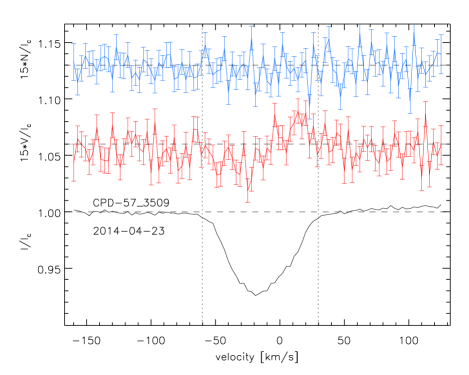
Figure 2: LSD profiles of Stokes $I$ (black solid line – bottom profile), $V$ (red solid line – middle profile), and $N$ parameter (blue solid line – top profile) obtained for CPD $-57^{\circ}$ 3509 in the Bonn reduction. The error bars of the LSD profiles are shown for both Stokes $V$ and the $N$ parameter. The vertical dotted lines indicate the velocity range adopted for the determination of the detection probability and magnetic field value. All profiles have been rigidly shifted upwards/downwards using arbitrary values and the Stokes $V$ and $N$ profiles have been expanded 15 times.

The value of the surface-averaged longitudinal magnetic field $\langle$B${}_{z}\rangle$ was calculated using either the hydrogen lines or the whole spectrum in the 3710–5870 Å spectral region. A summary of the results is shown in Table 1. The first column indicates the group, hence adopted data reduction and analysis, which obtained the results shown in the remaining columns. The heliocentric Julian date shown in Column 3 is that of the beginning of the sequence of exposures. Column 4 gives the number of frames obtained during each night of observation, while column 5 shows the exposure time, in seconds, of each frame. Column 6 gives the S/N per pixel of Stokes $I$ calculated at about 4950 Å over a wavelength range of 100 Å. Columns 7 and 8 give the $\langle$B${}_{z}\rangle$ values in Gauss, obtained using the spectral regions covered by the hydrogen lines obtained from the Stokes $V$ and $N$ parameter spectrum, respectively. The same is given in Columns 9 and 10, but using the entire spectrum.

Of the five FORS2 measurements, those obtained on the 7 February 2014, 2 June 2014, and 17 March 2015 led to a magnetic field detection, while we consistently found non-detections from the null profile (i.e. $\langle$N${}_{z}\rangle$ consistent with zero). The results from both independent data reductions and analyses are consistent within the mutual uncertainties.

3.2 HARPS observations

Like for the FORS2 data, the HARPSpol observations have been independently reduced by two different groups. The first reduction and analysis (Bonn) was performed with the reduce package (Piskunov & Valenti, 2002) and the least-squares deconvolution technique (LSD; Donati et al., 1997), while the second reduction and analysis (Potsdam) was performed with the ESO/HARPS pipeline and the LSD technique.

3.2.1 Bonn reduction and analysis

The one-dimensional spectra, obtained with reduce, were combined using the “ratio” method in the way described by Bagnulo et al. (2009). We then re-normalised all spectra to the intensity of the continuum obtaining a spectrum of Stokes $I$ ($I/I_{c}$) and $V$ ($V/I_{c}$), plus a spectrum of the diagnostic null profile ($N$ - see Bagnulo et al., 2009), with the corresponding uncertainties. The profiles of the Stokes $I$, $V$, and $N$ parameter were analysed using LSD, which combines line profiles (assumed to be identical) centred on the position of the individual lines and scaled according to the line strength and sensitivity to a magnetic field (i.e. line wavelength and Landé factor). We computed the LSD profiles of Stokes $I$, $V$ and of the null profile using the methodology and the code described in Kochukhov et al. (2010). We prepared the line mask used by the LSD code adopting the stellar parameters obtained from the spectroscopic analysis (see Sect. 4). We extracted the line parameters from the Vienna Atomic Line Database (vald; Piskunov et al., 1995; Kupka et al., 1999; Ryabchikova et al., 1999) and tuned the given line strength to the observed Stokes $I$ spectrum with the aid of synthetic spectra calculated with synth3 (Kochukhov, 2007). We used all lines deeper than 10% of the continuum, avoiding hydrogen lines, helium lines with developed wings, and lines in spectral regions affected by the presence of telluric features, 91 lines in total. We defined the magnetic field detection making use of the false alarm probability (FAP; Donati et al., 1992), considering a profile with FAP $<$ 10^-5 as a definite detection, $10^{-5}$ $<$ FAP $<$ $10^{-3}$ as a marginal detection, and FAP $>$ $10^{-3}$ as a non-detection.

The LSD profiles we obtained for CPD $-57^{\circ}$ 3509 are shown in Fig. 2, with the S/N of the LSD Stokes $V$ profile reaching 1342. The analysis of the Stokes $V$ LSD profile led to a clear, definite detection with a FAP = 9.4$\times$10^-7, while the analysis of the LSD profile of the null parameter led to a non-detection, $\left<N_{\rm z}\right>$ = 75$\pm$72 G with FAP $>$ 0.01. Integrating over a range of 90 $\mathrm{km\,s}^{-1}$ (i.e. $\pm$45 $\mathrm{km\,s}^{-1}$ from the line centre), we derived $\langle$B${}_{z}\rangle$ = $-$557$\pm$73 G. The measurements carried out with FORS2 and HARPS indicate the presence of a rather strong field with reversing polarity.

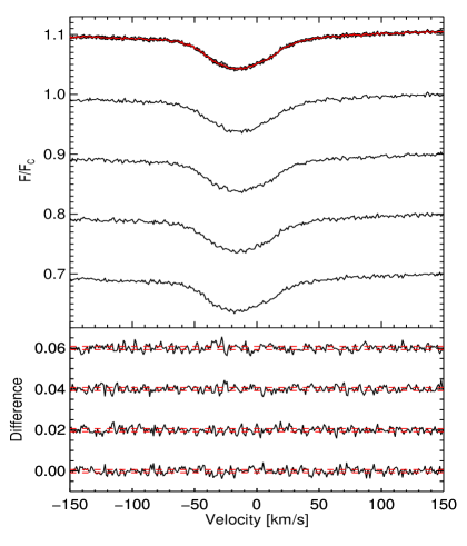
Figure 3: Testing for the presence of $\beta$ Cephei pulsations in CPD $-57^{\circ}$ 3509 on the basis of LSD Stokes $I$ profiles for the individual HARPS subexposures from the Potsdam reduction. The normalised average profile (in red, overlaid on all four sub-exposures in the topmost curve) and the individual subexposure profiles (subsequent curves) are shown in the upper panel, shifted by constant offsets. The lower panel shows the difference between the individual subexposures and the average profile, with the dashed lines indicating the $\pm$1$\sigma$-ranges.

3.2.2 Potsdam reduction and analysis

The reduction and calibration of the HARPS polarimetric spectra were performed using the HARPS data reduction software available at ESO’s 3.6 m telescope (La Silla, Chile). The normalisation of the spectra to the continuum level consisted of several steps described in detail by Hubrig et al. (2013). The Stokes $I$ and $V$ parameters were derived following Ilyin (2012), and null polarisation spectra were calculated by combining the subexposures in such a way that polarisation canceled out. These steps minimise spurious signals in the obtained data (e.g. Ilyin, 2012).

Since a number of magnetic Bp stars were reported to show $\beta$ Cephei-like pulsations (e.g. Neiner et al., 2012), and pulsations are known to have an impact on the analysis of the presence of a magnetic field and its strength (e.g. Schnerr et al., 2006; Hubrig et al., 2011a), we verified that no change in the line profile shape or radial velocity shifts are present in the obtained sub-exposures. We recall that the time elapsed between consecutive exposures is 45 minutes. On the one hand, this time scale is appropriate to detect $\beta$ Cep-like pulsations (which typically have periods of 4 hours, e.g. Stankov & Handler, 2005). On the other hand, the total time span (3 hours) is likely to be short enough to be free of the effects of the rotational modulation by spots. In Fig. 3 we present Stokes $I$ profiles computed for the individual subexposures. The line mask consisting of 163 He i and metal lines was constructed using the VALD database. The overplotted profiles are shown on the top, together with the average profile. The differences between the Stokes $I$ profiles computed for the individual sub-exposures and the average Stokes $I$ profile are presented in the lower panel. No impact of pulsations at a level higher than the spectral noise is detected, which is in line with the non-detection of photometric variations by Balona (1994) in his search for short period B-type variables in NGC 3293.

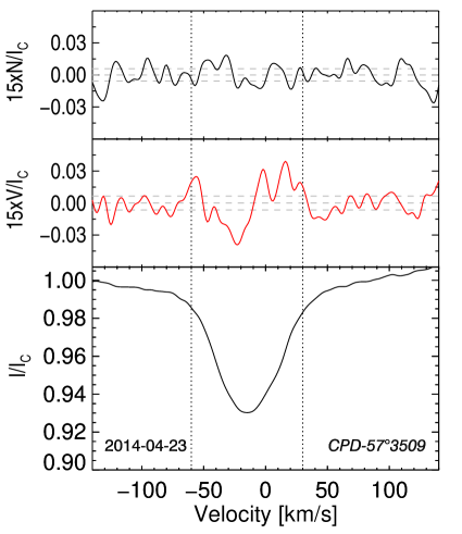
Figure 4: Same as Fig. 2, but for the Potsdam reduction. The horizontal dashed lines indicate the average values and the $\pm$1$\sigma$-ranges.

To search for the magnetic field, we employed an independent implementation of the LSD technique once more. The resulting mean LSD Stokes $I$, Stokes $V$, and diagnostic $N$ profiles obtained for the same line list as used for the search of the spectral variability are presented in Fig. 4. Using the FAP in the region of the whole Stokes $I$ line profile (velocity range from $-$60 km s^-1 to +30 km s^-1), we obtained a definite magnetic field detection $\left<B_{\rm z}\right>$ = $-$490$\pm$29 G with FAP = $1\times 10^{-10}$. The null parameter led to a non-detection, $\left<N_{\rm z}\right>$ = 34$\pm$50 G with FAP $=$ 0.024. We conclude that the two independent LSD analyses are consistent.

4 Model atmosphere analysis

4.1 Codes and analysis methodology

We employ a hybrid non-LTE approach for the model atmosphere analysis of CPD $-57^{\circ}$ 3509 (Nieva & Przybilla, 2007, 2012, henceforth abbreviated as NP12). Model atmospheres were computed with the Atlas9 code (Kurucz, 1993), which assumes plane-parallel geometry, chemical homogeneity, and hydrostatic, radiative, and local thermodynamic equilibrium (LTE). The model atmospheres were held fixed in the subsequent non-LTE line-formation calculations. Non-LTE level populations and model spectra were obtained with recent versions of Detail and Surface (Giddings, 1981; Butler & Giddings, 1985, both updated and extended by one of us (KB)). The coupled radiative transfer and statistical equilibrium equations were solved with Detail, employing the accelerated lambda iteration scheme of Rybicki & Hummer (1991). This allowed even complex ions to be treated in a realistic way. Synthetic spectra were calculated with Surface, using refined line-broadening theories. Continuous opacities due to hydrogen and helium were considered in non-LTE, and line blocking was accounted for via LTE opacity sampling, employing the method of Kurucz (1996). Microturbulence was considered in a consistent way throughout all computation steps: atmospheric structure computations, non-LTE level populations determination, and the formal solution.

The He-strong nature of CPD $-57^{\circ}$ 3509 precludes the use of existing model grids for chemically normal stars for the analysis. Instead, dedicated computations were required to constrain the atmospheric parameters and elemental abundances. Non-LTE level populations and the synthetic spectra of all elements were calculated using the suite of model atoms listed in Table 2. Updates of some of the published models were carried out by introducing improved oscillator strengths and collisional data. These model atoms were employed previously by NP12 for the analysis of a sample of normal early B-type stars in a parameter range similar to that expected for CPD $-57^{\circ}$ 3509. They were complemented by model atoms for additional trace species, which facilitated the determination of abundances for all elements detectable in the available high-resolution spectrum.

Table 2: Model atoms for non-LTE calculations.

Ion	Model atom
H	Przybilla & Butler (2004)
He i/ii	Przybilla (2005)
C ii/iii	Nieva & Przybilla (2006, 2008)
N ii	Przybilla & Butler (2001), updated
O ii	Becker & Butler (1988), updated
Ne i	Morel & Butler (2008), updated
Mg ii	Przybilla et al. (2001a)
Al iii	Przybilla (in prep.)
Si ii/iii/iv	Przybilla & Butler (in prep.)
S ii/iii	Vrancken et al. (1996), updated
Ar ii	Butler (in prep.)
Fe iii	Morel et al. (2006), corrected

In a first step, the hydrogen Balmer lines, the He i/ii lines, and additional ionization equilibria of C ii/iii, Si ii/iii/iv and S ii/iii were employed to constrain the atmospheric parameters – effective temperature $T_{\mathrm{eff}}$, (logarithmic) surface gravity $\log g$, microturbulence $\xi$, helium abundance $y$ (by number), projected rotational velocity $v\sin i$ and macroturbulent velocity $\zeta$ – in a similar approach to NP12. We use Spas (Spectrum Plotting and Analysing Suite, Hirsch, 2009) for the comparison of synthetic spectra with observations based on microgrids. Spas provides the means to interpolate between model grid points for up to three parameters simultaneously and allows instrumental, rotational, and (radial-tangential) macrobroadening functions to be applied to the resulting theoretical profiles. The program uses the downhill simplex algorithm (Nelder & Mead, 1965) to minimise $\chi^{2}$ in order to find a good fit to the observed spectrum. Once the atmospheric parameters were established, elemental abundances for the additional chemical species were determined using Spas. With the resulting abundances the entire process was iterated to account for the abundance effects on line blanketing and blocking.

Limitations.

The present approach does not account for phenomena like spots or vertical chemical stratification of the atmosphere, or for the effects of the magnetic field on the radiative transfer. Such effects are modelled occasionally using LTE techniques for spectrum synthesis on prescribed model atmospheres (e.g. Landstreet, 1988; Donati, 2001; Carroll et al., 2012), but non-LTE effects – which are important in early B-type stars (e.g. Nieva & Przybilla, 2007; Przybilla et al., 2011) – are just being considered (Yakunin et al., 2015). While the two available high-resolution spectra indicate the presence of surface spots because of the small-scale line-profile changes (see Fig. 1 for examples), the deviations from a homogeneous surface and resulting symmetric line profiles generally seem small, as implied by the good fit of the model to the FLAMES/GIRAFFE spectral snapshot (see Sect. 4.2). The issue may be revisited in greater detail once proper high-quality time series observations of the star become available.

Other effects that are not considered are the potential oblateness and gravity darkening in a fast-spinning star. Some He-strong stars are known to rotate near critical velocity (Grunhut et al., 2012; Rivinius et al., 2013), and the nightly variation in the magnetic field (Sect. 3) implies that CPD $-57^{\circ}$ 3509 is rotating at a much higher velocity than the observed rather low $v\sin i$ = 35 km s^-1 would suggest. The question is how close to critical velocity ($\sim$500 km s^-1 in this case) the star rotates, since significant effects on the atmospheric parameter and abundance determination are expected only for rotational velocities over 60% critical (Fremat et al., 2005). Assuming that CPD $-57^{\circ}$ 3509 is a magnetic oblique rotator, the observed change in polarity of the magnetic field implies that the equatorial rotational velocity should be in the range $\sim$70–250 km s^-1 assuming a one to three-day rotation period (see Sect. 5 for a discussion), so our present analysis approach seems adequate. However, a conclusive statement on this can only be given once the rotation period is firmly established.

Table 3: Parameters and elemental abundances of CPD $-57^{\circ}$ 3509.

Sp. Type	B2 IV He-strong
$v_{\mathrm{rad}}$	$-$16 … $-20$ km s-1
$d_{\mathrm{spec}}$	2630 $\pm$ 370 pc
$B_{\mathrm{d}}$	$\gtrsim$3300 G
Atmospheric parameters:
$T_{\mathrm{eff}}$	23750 $\pm$ 250 K
$\log g$ (cgs)	4.05 $\pm$ 0.10
$y$ (number fraction)	0.28 $\pm$ 0.02
$\xi$	2 $\pm$ 1 km s-1
$v\sin i$	35 $\pm$ 2 km s-1
$\zeta$	10 $\pm$ 2 km s-1
Non-LTE metal abundances:
$\log$(C/H) $+$ 12	8.37 $\pm$ 0.09 (5)
$\log$(N/H) $+$ 12	7.70 $\pm$ 0.07 (20)
$\log$(O/H) $+$ 12	8.65 $\pm$ 0.08 (36)
$\log$(Ne/H) $+$ 12	8.05 $\pm$0.15 (2)
$\log$(Mg/H) $+$ 12	7.17 (1)
$\log$(Al/H) $+$ 12	5.93 $\pm$ 0.07 (4)
$\log$(Si/H) $+$ 12	7.16 $\pm$0.05 (7)
$\log$(S/H) $+$ 12	7.17 $\pm$ 0.04 (4)
$\log$(Ar/H) $+$ 12	6.68 $\pm$ 0.04 (2)
$\log$(Fe/H) $+$ 12	7.30 $\pm$ 0.04 (6)
Photometric data:
$V$	10.68 $\pm$ 0.06 mag
$B-V$	0.10 $\pm$ 0.03 mag
$E(B-V)$	0.33 $\pm$ 0.03 mag
$M_{V}$	$-$2.47 $\pm$ 0.33 mag
$M_{\mathrm{bol}}$	$-$4.86 $\pm$ 0.33 mag
Fundamental parameters:
	Ekström et al. (2012)	Brott et al. (2011)
	tracks	tracks/Bonnsai
$M/M_{\odot}$	9.7$\pm$0.3	9.2$\pm$0.4
$R/R_{\odot}$	5.0$\pm$0.9	4.4${}^{+0.7}_{-0.5}$
$\log L/L_{\odot}$	3.85$\pm$0.13	3.76${}^{+0.12}_{-0.11}$
$\tau$	13.8${}^{+2.4}_{-3.3}$ Myr	13.0${}^{+1.7}_{-4.0}$ Myr
$\tau/\tau_{\mathrm{MS}}$	0.51${}^{+0.12}_{-0.16}$	0.47${}^{+0.13}_{-0.17}$

longtablel@ lrrlllr Spectral line analysis for CPD $-57^{\circ}$ 3509
Ion $\lambda\,$(Å) $\chi$ (eV) $\log gf$ Acc. Src. Broad. $\varepsilon_{\mathrm{NLTE}}(X)$
continued.
Ion $\lambda\,$(Å) $\chi$ (eV) $\log gf$ Acc. Src. Broad. $\varepsilon_{\mathrm{NLTE}}(X)$
C ii 3920.69 16.33 $-$0.232 B WFD C 8.32
C ii 4267.00 18.05 0.563 C+ WFD G 8.28
C ii 4267.26 18.05 0.716 C+ WFD G
C ii 4267.26 18.05 $-$0.584 C+ WFD G
C ii 6578.05 14.45 $-$0.087 C+ N02 C 8.31
C ii 6582.88 14.45 $-$0.388 C+ N02 C 8.48
C iii 4647.42 29.53 0.070 B+ WFD C 8.45
N ii 3955.85 21.15 $-$0.813 B WFD C 7.75
N ii 3995.00 18.50 0.163 B FFT C 7.60
N ii 4035.08 23.12 0.599 B BB89 C 7.79
N ii 4041.31 23.14 0.748 B MAR C 7.70
N ii 4043.53 23.13 0.440 C MAR C 7.73
N ii 4176.16 23.20 0.316 B MAR C 7.72
N ii 4179.67 23.25 $-$0.090 X KB C 7.81
N ii 4227.74 21.60 $-$0.060 B WFD G 7.71
N ii 4236.91 23.24 0.383 X KB C 7.59
N ii 4237.05 23.24 0.553 X KB C
N ii 4241.24 23.24 $-$0.337 X KB C 7.68
N ii 4241.76 23.24 0.210 X KB C
N ii 4241.79 23.25 0.713 X KB C
N ii 4242.50 23.25 $-$0.337 X KB C
N ii 4432.74 23.42 0.580 X KB C 7.63
N ii 4447.03 20.41 0.221 B FFT C 7.70
N ii 4530.41 23.47 0.604 C+ MAR C 7.65
N ii 4601.48 18.47 $-$0.452 B+ FFT C 7.75
N ii 4607.15 18.46 $-$0.522 B+ FFT C 7.69
N ii 4613.87 18.47 $-$0.622 B+ FFT C 7.80
N ii 4621.39 18.47 $-$0.538 B+ FFT C 7.67
N ii 4630.54 18.48 0.080 B+ FFT C 7.62
N ii 4643.08 18.48 $-$0.371 B+ FFT C 7.62
N ii 4694.64 23.57 0.100 X KB C 7.72
O ii 3911.96 25.66 $-$0.014 B+ FFT C 8.59
O ii 3912.12 25.66 $-$0.907 B+ FFT C
O ii 3945.04 23.42 $-$0.711 B+ FFT C 8.78
O ii 3954.36 23.42 $-$0.402 B+ FFT C 8.69
O ii 4069.62 25.63 0.144 B+ FFT C 8.57
O ii 4069.88 25.64 0.352 B+ FFT C
O ii 4072.72 25.65 0.528 B+ FFT C 8.74
O ii 4075.86 25.67 0.693 B+ FFT C 8.75
O ii 4078.84 25.64 $-$0.287 B+ FFT C 8.73
O ii 4129.32 25.84 $-$0.943 B+ FFT C 8.73
O ii 4132.80 25.83 $-$0.067 B+ FFT C 8.61
O ii 4156.53 25.85 $-$0.706 B+ FFT C 8.79
O ii 4185.45 28.36 0.604 D WFD C 8.52
O ii 4189.58 28.36 $-$0.828 D WFD C 8.54
O ii 4189.79 28.36 0.717 D WFD C
O ii 4317.14 22.97 $-$0.368 B+ FFT C 8.53
O ii 4319.63 22.98 $-$0.372 B+ FFT C 8.57
O ii 4325.76 22.97 $-$1.095 B FFT C 8.73
O ii 4349.43 23.00 0.073 B+ FFT C 8.67
O ii 4351.26 25.66 0.202 B+ FFT C 8.61
O ii 4351.46 25.66 $-$1.013 B FFT C
O ii 4366.89 23.00 $-$0.333 B+ FFT C 8.53
O ii 4369.28 26.23 $-$0.383 B+ FFT C 8.69
O ii 4414.90 23.44 0.207 B FFT C 8.62
O ii 4416.97 23.42 $-$0.043 B FFT C 8.67
O ii 4452.38 23.44 $-$0.767 B FFT C 8.63
O ii 4590.97 25.66 0.331 B+ FFT C 8.59
O ii 4595.96 25.66 $-$1.022 B FFT C 8.58
O ii 4596.18 25.66 0.180 B+ FFT C
O ii 4638.86 22.97 $-$0.324 B+ FFT C 8.68
O ii 4641.81 22.98 0.066 B+ FFT C 8.69
O ii 4649.13 23.00 0.324 B+ FFT C 8.74
O ii 4661.63 22.98 $-$0.269 B+ FFT C 8.69
O ii 4673.73 22.98 $-$1.101 B FFT C 8.71
O ii 4676.24 23.00 $-$0.410 B+ FFT C 8.69
O ii 4696.35 23.00 $-$1.377 B FFT C 8.62
O ii 4699.01 28.51 0.418 D WFD C 8.60
O ii 4699.22 26.23 0.238 B+ FFT C
O ii 4701.18 28.83 0.088 C WFD C 8.68
O ii 4703.16 28.51 0.262 D WFD C 8.69
O ii 4705.35 26.25 0.533 B+ FFT C 8.57
O ii 4710.01 26.23 $-$0.090 B+ FFT C 8.63
Ne i 6402.25 16.62 0.365 B+ FFT C 7.95
Ne i 6506.53 16.67 $-$0.002 B+ FFT C 8.16
Mg ii 4481.13 8.86 0.730 B+ FW G 7.17
Mg ii 4481.15 8.86 $-$0.570 B+ FW G
Mg ii 4481.33 8.86 0.575 B+ FW G
Al iii 4149.91 20.55 0.626 A+ FFTI C 5.99
Al iii 4149.97 20.55 $-$0.674 A+ FFTI C
Al iii 4150.17 20.56 0.471 A+ FFTI C
Al iii 4479.89 20.78 0.900 X KB C 5.93
Al iii 4479.97 20.78 1.020 X KB C
Al iii 4480.01 20.78 $-$0.530 X KB C
Al iii 4512.57 17.81 0.408 A+ FFTI C 5.96
Al iii 4528.95 17.82 $-$0.291 A+ FFTI C 5.83
Al iii 4529.19 17.82 0.663 A+ FFTI C
Si ii 3862.60 6.86 $-$0.757 C+ NIST C 7.08
Si ii 4128.05 9.84 0.359 B NIST LDA 7.15
Si iii 4552.62 19.02 0.292 B+ FFTI C 7.16
Si iii 4567.84 19.02 0.068 B+ FFTI C 7.19
Si iii 4574.76 19.02 $-$0.409 B FFTI C 7.25
Si iii 4716.65 25.33 0.491 B NIST C 7.15
Si iv 4116.10 24.05 $-$0.110 A+ FFTI D91 7.17
S ii 4162.67 15.94 0.78 D NIST C 7.19
S iii 3985.92 18.29 $-$0.79 E WSM C 7.22
S iii 4361.47 18.24 $-$0.39 D$-$ WSM C 7.14
S iii 4364.66 18.32 $-$0.71 E WSM C 7.14
Ar ii 4426.001 16.75 0.195 B+ FFTI C 6.65
Ar ii 4735.905 16.64 $-$0.096 B+ FFTI C 6.71
Fe iii 4081.01 20.63 0.372 X KB C 7.35
Fe iii 4164.73 20.63 0.923 X KB C 7.31
Fe iii 4310.36 22.87 1.156 X KB C 7.29
Fe iii 4310.36 22.87 0.189 X KB C
Fe iii 4372.04 22.91 0.585 X KB C 7.33
Fe iii 4372.10 22.91 0.029 X KB C
Fe iii 4372.13 22.91 0.727 X KB C
Fe iii 4372.31 22.91 0.865 X KB C
Fe iii 4372.31 22.91 0.193 X KB C
Fe iii 4372.50 22.91 0.200 X KB C
Fe iii 4372.54 22.91 0.993 X KB C
Fe iii 4372.78 22.91 0.040 X KB C
Fe iii 4372.82 22.91 1.112 X KB C
Fe iii 4419.60 8.24 $-$2.218 X KB C 7.25
Fe iii 4431.02 8.25 $-$2.572 X KB C 7.30

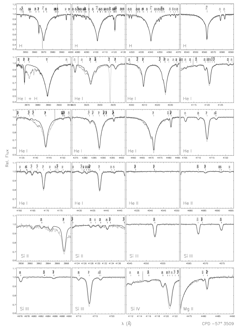
Figure 5a: Comparison of our global best-fit model (thick black line) to the normalised FLAMES/GIRAFFE spectrum of CPD $-57^{\circ}$ 3509 (grey line), concentrating here on H, He i/ii, Si ii/iii/iv and Mg ii lines. The panels are centred on analysed lines, sorted according to chemical species (as indicated in the lower left of each panel), and, within a species, sorted along increasing wavelength. Line identifications are given.

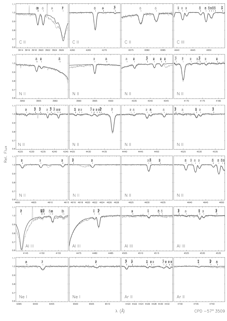
Figure 5c: Same as Fig. 5a, but for spectral lines of C ii/iii, N ii, Al iii, Ne i and Ar ii.

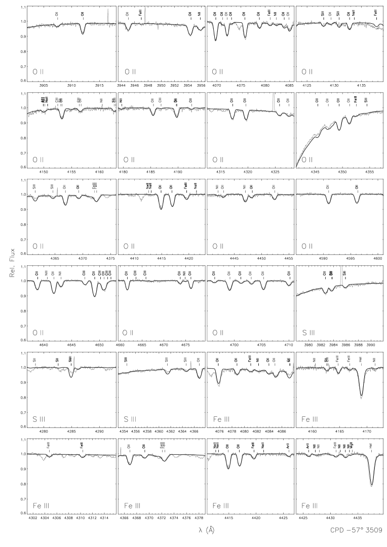
Figure 5d: Same as Fig. 5a, but for spectral lines of O ii, S ii/iii and Fe iii.

Figure 5: Elemental abundances in the atmosphere of CPD $-57^{\circ}$ 3509 relative to the cosmic abundance standard (CAS). The error bars show statistical 1$\sigma$-uncertainties from the line-to-line scatter in each element. Systematic uncertainties of the abundances amount to about 0.1 dex.

4.2 Results

Table 3 summarises the results from the comprehensive characterisation of CPD $-57^{\circ}$ 3509 as obtained in this work. A first block of entries gives the spectral type, the barycentric radial velocity $v_{\mathrm{rad}}$ (which is slightly variable among the available high-resolution spectra because of the presence of spots, and broadly consistent with the cluster $v_{\mathrm{rad}}$ of 12$\pm$5 km s^-1 as derived by Evans et al., 2005), the spectroscopic distance $d_{\mathrm{spec}}$ (following NP12), and the dipolar field strength $B_{\mathrm{d}}$ (assuming a dipolar field configuration, see Sect. 5 for a discussion). Then, the second and third blocks summarise the results of the quantitative analysis on atmospheric parameters and non-LTE metal abundances by number (the number of analysed lines is also indicated), respectively. Detailed information on the abundances derived for all diagnostic metal lines is given in Table 4.1, which is only available online. There, information on the transition wavelength $\lambda$, the excitation potential $\chi$ of the lower level of the transition, the oscillator strength $gf$, an indicator of its accuracy, the source of the $gf$-value, and a reference for the quadratic Stark broadening data employed for the computations is also summarised. The final elemental abundances were calculated giving equal weight to all lines from all ions of a chemical species, the uncertainties in Table 3 representing the 1$\sigma$ standard deviations from the line-to-line scatter. Systematic errors due to factors like uncertainties in stellar parameters, continuum setting, and atomic data on the elemental abundances are difficult to quantify accurately (see e.g. Sigut, 1999; Przybilla et al., 2001a, b). From these previous experiences, we expect them to amount to about 0.1 dex.

A comparison of the synthetic spectrum based on the parameters from Table 3 with the observed FLAMES/GIRAFFE spectrum is shown in Figs. 5a-5d (the last two available in the online version of the paper) on a line-by line basis. Figure 5a concentrates on the hydrogen Balmer lines, the unusually strong helium lines that are characteristic of the He-strong stars, and the Si ii-iv lines. Overall, a good fit between model and observation is achieved. The unmodelled narrow extra absorption close to the core of H$\epsilon$ is the interstellar Ca H line. Some slightly blueshifted excess absorption is noticeable mostly in several of the He i lines. This feature is likely due to a spot on the surface. (Similar signatures can also be seen on a much smaller scale in some metal lines.) It is not clear whether vertical chemical stratification is an issue here, because clear-cut signatures such as core-wing anomalies (e.g. Maza et al., 2014) are absent. We note that the poor fit to some of the He i lines like $\lambda\lambda$ 3926 Å and 4141/4143 Å, or even their absence from the model ($\lambda$ 3871 Å), is because of the lack of appropriate broadening data in the literature.

A proper determination of the atmospheric indicators is further indicated by the match of four ionization balances simultaneously, He i/ii, C ii/iii, Si ii-iv, and S ii/iii (Figs. 5a-5d). The strongest constraints stem from silicon, which covers both the main and the two adjacent minor ionisation stages. The presence of He ii at such a low $T_{\mathrm{eff}}$ in a main-sequence star is unusual, but results from the high helium abundance. The overall good to excellent match of the metal line profiles by theory – also for species where only lines from one ion are observed – reflects the small dispersion in abundances. To our knowledge, this represents the most comprehensive non-LTE abundance study of any He-strong star to date.

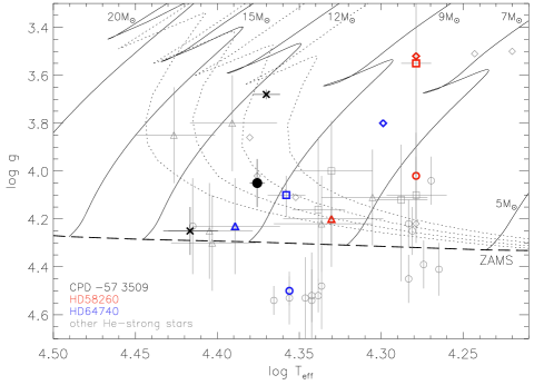
Figure 6: CPD $-57^{\circ}$ 3509 in the $\log T_{\mathrm{eff}}$-$\log g$ diagram (black dot, this work). Previous analysis results of the star obtained by use of grids assuming solar helium abundance are indicated by St. Andrew’s crosses, from the work by Hunter et al. (2009, high-gravity solution) and McSwain et al. (2009, low-gravity solution). Analysis results for other He-strong stars from the literature are also shown from Zboril et al. (1997, circles), Leone et al. (1997, diamonds), Hunger & Groote (1999, squares), and Cidale et al. (2007, triangles), marked in grey. Two stars common to all four analyses are highlighted, HD 58260 (red symbols) and HD 64740 (blue symbols). Where available, 1$\sigma$ error bars are displayed. Overlaid are Geneva evolution tracks for rotating stars, computed for metallicity $Z$ = 0.014 and an initial value of 40% of the critical rotation rate (Ekström et al., 2012, full lines). Corresponding isochrones for $\log\tau$ (Myr) = 7.0, 7.1, 7.2, and 7.3 are also displayed (dotted lines), as well as the position of the zero-age main sequence (ZAMS, long-dashed line).

The resulting abundance pattern with respect to the cosmic abundance standard (CAS), as established from early B-type stars in the solar neighbourhood (Nieva & Przybilla, 2012; Przybilla et al., 2013, preliminary values for Al, S and Ar are adopted from the latter work), is presented in Fig. 5. The common bracket notation is used: $[$El/H$]$ = $\log$ (El/H) $-$ $\log$ (El/H)_CAS. Besides the high value for helium, a bimodal behaviour is found for the metal abundances. A group of elements (C, N, O, Ne, S, Ar) shows abundances close to CAS values, while another group (Mg, Al, Si, Fe) is deficient by a factor $\sim$2. The first group of elements seems to be close to the pristine abundances of the NGC 3293 cluster, which lies at a Galactocentric distance only $\sim$300 pc smaller than that of the Sun; i.e., CAS values should be representative in the absence of azimuthal abundance variations.

The fourth block of Table 3 concentrates on photometric data for CPD $-57^{\circ}$ 3509. The observed Johnson $V$ magnitude and $B-V$ colour are adopted from Delgado et al. (2011). The colour excess $E(B-V)$ was determined by comparison with synthetic photometry from the Atlas9 flux. Correction for extinction (assuming a ratio of total-to-selective extinction $R_{V}$ = 3.1) allows the absolute visual magnitude $M_{V}$ to be derived for the spectroscopic distance, and application of the bolometric correction from the Atlas9 model allows the bolometric magnitude $M_{\mathrm{bol}}$ to be determined.

Finally, the fundamental stellar parameters mass $M$, radius $R$, luminosity $L$, evolutionary age $\tau$ and fractional main-sequence lifetime $\tau/\tau_{\mathrm{MS}}$ were derived via comparison with stellar evolution models from the Geneva group (Ekström et al., 2012), as summarised in the last block of Table 3. The location of the star in the $\log T_{\mathrm{eff}}$-$\log g$ plane (Fig. 6) with respect to the evolutionary tracks and isochrones provided the evolutionary mass, age, and fractional main-sequence age, respectively. Luminosity and radius followed, once the (spectroscopic) distance was determined. A second independent derivation of the fundamental parameters employed the Bayesian statistical tool Bonnsai (Schneider et al., 2014) on the basis of stellar evolution tracks by Brott et al. (2011). A Salpeter mass function was adopted as prior for the initial stellar masses, a Gaussian rotational velocity distribution with mean of 100 km s^-1 and FWHM of 250 km s^-1 (cf. Hunter et al., 2008) and a uniform prior in age. Furthermore, it was assumed that all rotation axes are randomly oriented in space. The offset between the two solutions – though being within the mutual uncertainties – is mostly related to the higher overshooting value adopted in the Brott et al. (2011) models. For test purposes, a bi-modal rotational velocity distribution as derived by Dufton et al. (2013) was also employed as prior in the Bonnsai modelling, resulting in practically identical fundamental stellar parameters as reported in Table 3. For further tests with Bonnsai, we also assumed the star to be an intrinsic faster rotator, adopting $v_{\mathrm{rot}}$ = 200$\pm$50 km s^-1. A slight trend is found that we would overestimate the age and underestimate the mass of the star in that case, however with the changes covered well by the uncertainties stated in Table 3.

The fundamental stellar parameters may be subject to some additional systematic error. This is because of the chemically normal interior of the star (see Sect. 5) and the chemically peculiar atmosphere, which is not reflected by the evolution models; i.e., the surface parameters predicted by the models are slightly different than those observed. However, we expect this to be a secondary effect only, which is confirmed by the rather good match of the stellar values with the NGC 3293 cluster distance and age of $\sim$2460 pc and 10.7 Myr as discussed, for example, by Lotkin & Matkin (1994).

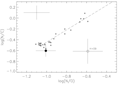
Figure 7: Position of CPD $-57^{\circ}$ 3509 in the N/O-N/C diagram (by mass): present work (black dot) and the result from Hunter et al. (2009, open circle), compared to 29 early B-type stars from Nieva & Simón-Díaz (2011) and NP12 (grey dots). An error bar typical for the latter is indicated in the upper left corner. The dashed line indicates the analytical approximation to the nuclear path for CN-cycled material using CAS values (Przybilla et al., 2010).

4.3 Comparison with previous work

The same FLAMES/GIRAFFE spectrum of CPD $-57^{\circ}$ 3509 was analysed previously by Hunter et al. (2009). Their $T_{\mathrm{eff}}$ of 26 100$\pm$1000 K and $\log g$ = 4.25$\pm$0.10 differ significantly from our solution, a result of the assumption of a solar helium abundance in their analysis. All other atmospheric parameters and the metal abundances in common (C, N, Mg, Si) are rather close to our results, which is very likely an effect of cancellation of several factors. An exception is oxygen, for which they indicate an abundance lower by more than 0.5 dex.

Confidence in our solution also comes from a better match of the position of CPD $-57^{\circ}$ 3509 in the N/C vs. N/O diagram with respect to the predicted nuclear path, which provides a powerful quality test for observational results (Przybilla et al., 2010; Maeder et al., 2014), see Fig. 7. The current position of CPD $-57^{\circ}$ 3509 in the diagram may not reflect its pristine position exactly because of the fractionated stellar wind. However, we expect systematic effects on the CNO ions to be small because of their similar atomic structures, similar atomic weights, and double-ionization energies near or above the He i edge; i.e., their relative abundances should not change much.

CPD $-57^{\circ}$ 3509 was also analysed by McSwain et al. (2009), based on lower-resolution spectra ($R$ $\approx$ 1500–4000). They found $T_{\mathrm{eff}}$ = 23 450$\pm$450 K and $\log g$ = 3.68$\pm$0.02 from interpolation of the Tlusty BSTAR2006 grid of Lanz & Hubeny (2007) aiming at minimisation of the root-mean-square difference between model and observation for a single line indicator, H$\gamma$. Their $v\sin i$ = 62$\pm$13 km s^-1 is a result of concentrating on He i lines in their analysis, which resulted in a higher $v\sin i$-value because the He-strong nature of the star was not recognised. The positions of CPD $-57^{\circ}$ 3509 for both the solutions by McSwain et al. (2009) and Hunter et al. (2009) are indicated in Fig. 6.

5 Discussion

Between the FORS2 (considering the whole spectrum) and HARPSpol observations, the highest $\langle$B${}_{z}\rangle$ value in modulus was obtained from the analysis of the FORS2 data obtained on 2 June 2014. Considering then $\langle$B${}_{z}\rangle$_max $\sim$ 1 kG and assuming a dipolar configuration of the magnetic field, we derive a lower limit on the dipolar field strength of B_d $\gtrsim$ 3.3 kG, following Aurière et al. (2007, their Sect. 2.7). In addition, the large and fast (within about 1 day) variation in the $\langle$B${}_{z}\rangle$ value shown by the analysis of the FORS2 data indicates that the star is rotating faster than implied by the low $v\sin i$-value with a likely rotation period of a few days or less. An estimate can be achieved from $v_{\mathrm{rot}}$ = $2\pi R/P$, assuming a rotation period $P$ in the range one to three days and adopting the range in radius, 4.4 to 5.0 $R_{\odot}$, obtained from considering the Geneva and Bonn models. One finds $v_{\mathrm{rot}}$ $\approx$ 70 to 250 km s^-1, so less than about 50% of the critical velocity. This may be viewed as an upper limit since the magnetic field geometry could be more complex than dipolar. An inclination angle $i$ in the range $\sim$8 to 30^∘ is implied.

From the magnetic field variations, we get values between $-$560 G and +1050 G (from the Bonn reduction). Since we do not have the fully modulated magnetic field variation curve, we do not know the real $\langle$B${}_{z}\rangle$_min and $\langle$B${}_{z}\rangle$_max. But if we use the measured values, we get $\langle$B${}_{z}\rangle$_min/$\langle$B${}_{z}\rangle$_max $=$ $-$0.53, $\beta$ = 88^∘ for $i$ = 8^∘, and $\beta$ = 80^∘ for $i$ = 30^∘, with $\beta$ being the obliquity angle, i.e. the angle between the rotation axis and the magnetic axis (see e.g. Sect. 3 of Hubrig et al. (2011b) for the formalism employed here). Of course, if the maximum/minimum values of $\langle$B${}_{z}\rangle$ differ significantly from the assumed values, $\beta$ will also change dramatically. And if we were looking equator-on, meaning that $\sin i$ = 1, it would be more difficult to make a statement about $\beta$. However, a $\beta$ close to 0^∘ is highly unlikely. To summarise here, a low inclination value combined with a high obliquity angle offers a plausible explanation for the apparent contrast between the small width of the absorption lines and the short timescale of the variation in the observed magnetic field strength.

In the context of the classification of magnetospheres of massive stars presented by Petit et al. (2013) and assuming a minimum dipolar magnetic field strength of 3.3 kG, we obtained a lower limit on the Alfvén radius of about 35 stellar radii and an upper limit on the Keplerian corotation radius of about 7 stellar radii. For the calculation of the Alfvén and Keplerian corotation radius we adopted the stellar parameters obtained from Bonnsai as presented in Table 3, a terminal velocity of 700 $\mathrm{km\,s}^{-1}$, and mass-loss rate $\dot{M}$ in the range of 10^-11 to 10^-10 $M_{\odot}$ yr^-1 typical of weak winds of magnetic B dwarfs (Oskinova et al., 2011).

The derived values indicate that the star should be able to support a centrifugal magnetosphere. The star could therefore hold a circumstellar disk or cloud formed of stellar wind material trapped within the magnetic field lines, which usually reveals itself by emission, for example in the H$\alpha$ line. The spectra collected so far do not present any signature indicative of the presence of circumstellar material. CPD $-57^{\circ}$ 3509 therefore seems to be one of the examples of He-strong stars with H$\alpha$ absorption, similar to HD 58260 (Pedersen, 1979) or HD 96446 (Neiner et al., 2012), which indicate that a centrifugal magnetosphere is a necessary but not sufficient condition for developing emission.

Apparently, the wind is either not strong enough for sufficient material to accumulate in the magnetosphere to become observable, or alternatively, some leakage process leads to loss of material from the magnetosphere (see Petit et al. (2013) for further discussion). One may speculate that the magnetic field topology, in particular deviations from a global dipole that can favour magnetic reconnection, may play a rôle in such a leakage process by weakening the magnetic confinement of the circumstellar material. Alternatively, a high obliqueness of the magnetic field with respect to the rotation axis may inhibit the formation of a circumstellar disk, since mass loss into some solid angle can occur along field lines in the equatorial plane in that case.

Once considered a small number of oddballs, it is now clear that He-strong stars compose an important second class of magnetic objects among massive stars, easily identified spectroscopically like the magnetic Of?p stars. Their quantitative analysis, like that for any chemically-peculiar object, is more demanding than for ordinary stars. That said, it seems that the atmospheric parameters of the He-strong stars are rather poorly constrained, since huge systematics between different studies of the same star are apparent (see Fig. 6). Essentially, any position from close to the zero-age main sequence (ZAMS) to near the end of core hydrogen burning, and even below the ZAMS, has been assigned to some prototype objects of this class in several previous studies. Also, differences in $T_{\mathrm{eff}}$ can be considerable. Further studies with modern non-LTE modelling techniques, as applied here, are certainly needed to improve our understanding of this class of star. In particular, it is imperative to account for the peculiar helium abundances in the modelling, because its neglect can lead to large systematic effects on the analysis, see the discussion in Sect. 4.3.

The helium abundance of $y$ = 0.28 (which corresponds to a mass fraction of 0.6) in the atmosphere of CPD $-57^{\circ}$ 3509 locates the star in the upper quartile of the helium abundance distribution for He-strong stars (Zboril et al., 1997). Given the star’s luminosity of $\log L/L_{\odot}$ $\approx$ 3.8 one can conclude that the He enrichment is indeed confined to the atmospheric layers, and the envelope has normal He composition: if the He mass fraction inside the star were as high as 0.6, then its luminosity would have to be much higher: $\log L/L_{\odot}$ = 4.2, according to the mass-luminosity-helium mass fraction relation (Gräfener et al., 2011).

Non-LTE abundances for all elements with lines in the optical spectra in early B-stars were derived here for the first time for a He-strong star. It is therefore worthwhile discussing the resulting abundance pattern for CPD $-57^{\circ}$ 3509 (Fig. 5) further. It is probably a consequence of the fractionated stellar wind that also gives rise to the peculiarity in helium abundance (Hunger & Groote, 1999; Krtička & Kubát, 2001). The weak wind prevailing at the $T_{\mathrm{eff}}$ of CPD $-57^{\circ}$ 3509 is radiatively driven by metal species with pronounced line spectra longwards of the Lyman jump, i.e. those that can efficiently absorb momentum from the radiation field near maximum flux. Good examples for these are silicon and iron. All other elements we analysed show a relatively sparse line density and typically weak lines, so they participate in the outflow by being accelerated indirectly via Coulomb collisions, like hydrogen. As they are typically ionized singly, they do not decouple from the outflow and fall back to the surface like neutral helium (part of the helium remains ionized and consequently gets dragged along with the stellar wind). More detailed investigations are required for magnesium and aluminium, but one may speculate that their observed underabundances may be the result of the stronger Coulomb coupling, because they are predominantly doubly ionized (both also show a few strong lines in the UV). This picture allows the prediction that other iron-group species that have an electron configuration with a partially filled 3$d$ valence shell similar to iron (and similar ionization energies) should also show underabundances by a factor $\sim$2 relative to cosmic values, which could be verified by UV spectroscopy.

One may assume that the abundances of helium and of the metals vary as a function of time in He-strong stars as they evolve off the ZAMS. The helium abundance would be expected to increase with time (due to fall-back), while the metal abundances should decrease (due to the fractionated, metal-rich wind). Quantifying the behaviour of $y(t)$ and $\log$(X/H) $[t]$ is not straightforward and would require computations like those of Michaud et al. (1987) to be undertaken, refined by modern input physics, but this is beyond the scope of the present paper. While observational evidence for this time-dependent behaviour is weak at best at present (see the discussion by Zboril et al., 1997) because of large observational uncertainties, applying the analysis methods presented here to a sample of He-strong stars may be worthwhile in order to investigate the question once again.

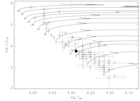
Figure 8: Massive stars with confirmed magnetic field detections in the Hertzsprung-Russell diagram (Briquet et al., 2013; Petit et al., 2013; Alecian et al., 2014; Neiner et al., 2014; Fossati et al., 2014, 2015a; Sikora et al., 2015; Castro et al., 2015, grey circles), and CPD $-57^{\circ}$ 3509 (black dot). Error bars are 1$\sigma$ uncertainties. Evolutionary tracks of Brott et al. (2011) for initial rotational velocity of $\sim$300 km s^-1 are shown (full lines), labelled by initial stellar mass. The magnetic star in the Trifid nebula and HD 345439 (Hubrig et al., 2014, 2015b) are not included here because of difficulties in establishing their properties.

Finally, we want to discuss the evolutionary status of CPD $-57^{\circ}$ 3509. Its position in the Hertzsprung-Russell diagram (HRD) is shown in Fig. 8 with respect to other currently known magnetic massive stars. Noteworthy is the good consistency of the star’s position in the HRD and the $T_{\mathrm{eff}}$-$\log g$ diagram (Fig. 6) relative to the stellar evolution tracks, despite the different sources of the tracks. It has evolved significantly away from the ZAMS, having burned about half of its core hydrogen. The star is close to the point where evolution speeds up towards the terminal-age main sequence and – given the uncertainties among previous studies – among the most evolved He-strong stars known, see Fig. 6. This is consistent with an evolutionary age (see Table 3) that compares reasonably well with the age of the parent open cluster NGC 3293, 10.7 Myr (Lotkin & Matkin, 1994). There is also reasonably good agreement between the spectroscopic distance of CPD $-57^{\circ}$ 3509 ($d_{\mathrm{spec}}$ = 2630$\pm$370 pc) and the cluster distance of $\sim$2460 pc (Lotkin & Matkin, 1994). By adopting this cluster distance and the values for reddening and bolometric correction determined here, one obtains an independent $\log L/L_{\odot}$ = 3.77, in excellent agreement with both our values derived from the Ekström et al. (2012) and Brott et al. (2011) tracks.