A study on conserving invariants of the Vlasov equation in semi-Lagrangian computer simulations

Abstract

The semi-Lagrangian discontinuous Galerkin method, coupled with a splitting approach in time, has recently been introduced for the Vlasov–Poisson equation. Since these methods are conservative, local in space, and able to limit numerical diffusion, they are considered a promising alternative to more traditional semi-Lagrangian schemes. In this paper we study the conservation of important physical invariants and the long time behavior of the semi-Lagrangian discontinuous Galerkin method. To that end we conduct a theoretical analysis and perform a number of numerical simulations. In particular, we find that the entropy is nondecreasing for the discontinuous Galerkin scheme, while unphysical oscillations in the entropy are observed for the traditional method based on cubic spline interpolation.

1 Introduction

The so-called semi-Lagrangian methods constitute a class of numerical schemes used to discretize hyperbolic partial differential equations (usually first order equations). The basic idea is to follow the characteristics backward in time. For the Vlasov–Poisson equation the characteristics corresponding to the splitting sub-steps can be determined analytically (as has been suggested in the seminal paper of Cheng & Knorr (1976)). However, since the endpoint of a characteristic curve does not necessarily coincide with the grid used, an interpolation procedure has to be employed. An obvious choice is to reconstruct the desired function by spline interpolation, which according to E. Sonnendrücker (2011) is still considered the de facto standard in Vlasov simulations. A downside of this approach is that a tridiagonal linear system of equations has to be solved to construct the spline. This algorithm has a low flop/byte ratio and significant communication overhead (both of which are unfavorable on most modern and future high performance computing systems).

On the other hand, the semi-Lagrangian discontinuous Galerkin method employs a piecewise polynomial approximation in each cell of the computational domain (Qiu & Shu, 2011; Rossmanith & Seal, 2011; Crouseilles et al., 2011b; Einkemmer & Ostermann, 2014b). In case of the advection equation the discretized function is translated and then projected back to the appropriate subspace of piecewise polynomial functions. This method, per construction, is mass conservative and only accesses two adjacent cells in order to compute the necessary projection (this is true independent of the order of the approximation). Furthermore, from the literature available it seems that the semi-Lagrangian discontinuous Galerkin method compares favorable with spline interpolation. In addition, mathematical rigorous convergence results are available (Einkemmer & Ostermann, 2014c, b).

A further method that has been widely employed in plasma simulations is the van Leer scheme (see, for example, Fijalkow (1999); Mangeney et al. (2002); Galeotti & Califano (2005); Valentini et al. (2005); Califano et al. (2006); Galeotti et al. (2006)). This case is formally similar to the discontinuous Galerkin scheme employed in this paper. What distinguishes the discontinuous Galerkin method from the van Leer scheme is that the coefficients in the corresponding basis expansion are stored directly in computer memory. In contrast, the van Leer scheme replaces these coefficients by performing an approximation using suitable differences on an equidistant grid.

The semi-Lagrangian discontinuous Galerkin scheme is fully explicit (i.e. no linear system has to be solved to advance the solution in time) and thus it is easier to implement (especially on parallel architectures) and shows a more favorable communication pattern. We should note that some measures have been taken to improve the parallel scalability of the cubic spline interpolation (Crouseilles et al., 2009a). However, even for this approach a relatively large communication overhead is incurred. This is due to the fact that the boundary condition for the local spline reconstruction requires a large stencil if the desirable properties of the global cubic spline interpolation are to be preserved (the method derived in Crouseilles et al. (2009a) requires a centered stencil of size $21$).

It is well known that the Vlasov–Poisson equation conserves a number of physically important variables. In many applications it is important that these quantities are conserved by the discretization (at least up to some tolerance; ideally up to machine precision) for long time intervals. For the cubic spline interpolation, which is employed in a number of software packages that are used to simulate the Vlasov equation, the good long time behavior is well established (even though there are no rigorous results). Furthermore, the conservation of invariants has been studied extensively for the (mostly second and third order) van Leer schemes. In Mangeney et al. (2002) the diffusive and dispersive error has been investigated and compared to spline interpolation. In Galeotti & Califano (2005) and Califano et al. (2006) particular emphasis has been placed on the diffusive behavior of the van Leer schemes and spline interpolation (which is of paramount importance for collisionless plasma simulations).

While some short time numerical results with respect to the conservation properties are available for the discontinuous Galerkin semi-Lagrangian method (Qiu & Shu, 2011; Crouseilles et al., 2011b), to the knowledge of the author no systematic study has been performed. Thus, the purpose of this paper is to investigate the performance of the semi-Lagrangian discontinuous Galerkin scheme with respect to the conservation of a number of physically important variables. We will also present long time integration results which so far have, to our knowledge, been absent from the literature. In addition, we investigate what effect the degree of the polynomial approximation has in this context. This is particular important for the discontinuous Galerkin approach as choosing a higher order approximation reduces the number of cells available in the numerical simulation.

In section 2 we introduce the Vlasov–Poisson equation, the splitting approach used for the time discretization, and both the semi-Lagrangian discontinuous Galerkin method as well as the semi-Lagrangian method based on the cubic spline interpolation. In section 3 we analyze the discontinuous Galerkin approach from a theoretical point of view and compare it to the cubic spline interpolation. This allows us to better understand the numerical results that have been obtained in section 4. In this section we provide results that compare the discontinuous Galerkin approach with the cubic spline interpolation and perform long time simulations in order to show the viability of the semi-Lagrangian discontinuous Galerkin scheme for the present application. Finally, we conclude in section 5.

2 Equations and numerical methods

In astro- and plasma physics the behavior of a collisionless plasma is modeled by the Vlasov equation

$$\partial_{t}f(t,x,v)+v\cdot\nabla f(t,x,v)+F\cdot\nabla_{v}f(t,x,v)=0,$$

which is posed in an up to $3+3$ dimensional phase space (although lower dimensional models are often employed as well). The variable $x$ denotes the position and variable $v$ denotes the velocity. The density function $f$ is the sought-after particle distribution and the (force) term $F$ describes the interaction of the plasma with the electromagnetic field. Depending on the application this force term can include the full Lorentz force or only the force due to the electric field.

In this paper we will restrict ourselves to the Vlasov–Poisson equation, i.e. the force term is given by $F=E$ and the electric field is determined by solving

$$\nabla\cdot E=\rho(x)-1,\qquad\nabla\times E=0$$

with charge density

$$\rho(x)=\int f(t,x,v)\,\mathrm{d}v.$$

In addition, in all our simulations we impose periodic boundary conditions in both the $x$- and $v$-directions.

To advance the numerical solution in time we use the splitting approach introduced in Cheng & Knorr (1976). That is, we consider (the first part of the splitting algorithm)

$$\partial_{t}f(t,x,v)+v\cdot\nabla f(t,x,v)=0,\qquad f(0,x,v)=g(x,v)$$ (1)

and denote the corresponding solution at time $\tau$ by

$$\mathrm{e}^{\tau A}g(x,v)=f(\tau,x,v).$$

For the second part of the splitting algorithm we then consider

$$\partial_{t}f(t,x,v)+E^{n}\cdot\nabla_{v}f(t,x,v)=0,\qquad f(0,x,v)=g(x,v),$$ (2)

where the electric field $E^{n}$ is determined from the density

$$\rho^{n}(x)=\int g(x,v)\,\mathrm{d}v$$

and is thus taken constant during each time step. We denote the corresponding solution by

$$\mathrm{e}^{\tau B}g(x,v)=f(\tau,x,v).$$

Note that, contrary to what the notation suggests, $B$ is a nonlinear operator as the electric field depends on the density function $f$. Using the introduced notation we can easily formulate a time step of the splitting algorithm. The Lie splitting

$$f^{n+1}(x,v)=\mathrm{e}^{\tau B}\mathrm{e}^{\tau A}f^{n}(x,v),$$

where $f^{n}$ is an approximation of $f(t_{n},x,v)$ and $\tau=t_{n+1}-t_{n}$ is the time step size, is a first order method. In all our simulation we will use the Strang splitting scheme

$$f^{n+1}(x,v)=\mathrm{e}^{\frac{\tau}{2}A}\mathrm{e}^{\tau B}\mathrm{e}^{\frac{\tau}{2}A}f^{n}(x,v)$$

which is a second order method and has roughly the same computational cost as the Lie splitting scheme. Let us also note that high order splitting methods have been constructed (Crouseilles et al., 2011a).

The main computational advantage of the splitting scheme is that the resulting sub-steps, given by (1) and (2), are in the form of an advection equation, where the advection speed is independent of the variable in the direction of the advection. Thus, we can immediately solve (1) to obtain

$$\mathrm{e}^{\tau A}g(x,v)=g(x-\tau v,v)$$ (3)

and (2) to obtain

$$\mathrm{e}^{\tau B}g(x,v)=g(x,v-\tau E(x)),$$ (4)

where $E$ is the electric field determined from the charge density corresponding to $g(x,v)$. Thus, by using the splitting approach outlined above we have reduced the task of computing a numerical approximation to the Vlasov–Poisson equation to computing two translations in phase space.

Now, up to this point phase space is still continuous. However, in order to implement the numerical scheme on a computer, we have to perform a space discretization that represents the numerical solution, at a fixed time step, using a finite number of degrees of freedom. The most straightforward approach is to choose a uniform grid. However, for any grid $(x_{i},v_{j})$ the translations $x_{i}-\tau v_{j}$ and $v_{j}-\tau E(x_{i})$, in general, do not coincide with a grid point. Thus, we have to use an interpolation scheme in order to evaluate $g(x_{i}-\tau v_{j})$ and $g(v_{j}-\tau E(x_{i}))$. In the Vlasov community interpolation based on cubic splines is very popular. This method is illustrated in figure 1 and proceeds in two steps:

1. construct a cubic spline using the known value of the function on the grid points (this involves the solution of a tridiagonal system of equations);

2. translate each grid point according to (3) or (4) and use the cubic spline to obtain the new value at that grid point.

Since we follow the characteristics backward in time (i.e. track particles along their trajectories) but use an Eulerian grid for the space discretization, these methods are usually referred to as semi-Lagrangian and are free of a Courant–Friedrichs–Lewy (CFL) condition. In addition, they do not exhibit the numerical noise that is prevalent in particle methods (such as the popular particle in cell scheme).

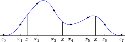
Figure 1: An illustration of the semi-Lagrangian method based on a quadratic spline interpolation is shown. In this case a continuous piecewise polynomial interpolant is constructed that is used for all evaluations. We illustrate three evaluations of the interpolant (denoted by the variable $x$).

For the Vlasov–Poisson equation it is vital that charge (or mass; the two quantities are equivalent as all particles in the physical model carry the same amount of electrical charge) is conserved. It is, a priori, not clear that the a semi-Lagrangian scheme based on spline interpolation satisfies this constraint. In order to show this, we reformulate the numerical method as a forward semi-Lagrangian scheme (as is done in Crouseilles et al. (2009b)). Since our interpolant is a cubic spline, we can expand $f^{n}(x,v)$ in the B-spline basis (for simplicity we restrict ourselves to the 1+1 dimensional case here)

$$f^{n}(x,v)=\sum_{kl}\omega_{kl}^{n}S(x-x_{k})S(v-v_{l}),$$

where $S$ is given by

$$6S(x)=\begin{cases}4-6(x/h)^{2}+3|x/h|^{3}&0\leq|x|\leq h\\ (2-|x/h|)^{3}&h\leq|x|\leq 2h\\ 0&\text{otherwise}\end{cases}$$

and $h$ is the grid spacing. The coefficients $\omega_{kl}^{n}$ are determined uniquely by the function values at the grid points but in order to obtain them we have to solve a linear system of equations. The forward semi-Lagrangian method based on cubic spline interpolation for (3) is then given by

$$f^{n+1}(x_{i},v_{j})=\sum_{kl}\omega_{kl}^{n}S(x_{i}-\tau v_{j}-x_{k})S(v_{j}-v_{l}).$$

For the constant advection case considered here this is merely a reformulation of the previously introduced (backward) semi-Lagrangian method. However, the interpretation is different (translating the basis function vs following the characteristics backward in time). That the forward semi-Lagrangian scheme is mass conservative can be easily deduced from the present formulation. First, we note that the B-splines form a partition of unity. That is, for all $x$ we have

$$\sum_{k}S(x-x_{k})=1.$$

Therefore, we can write the integral over a spline $u$ as follows

$$\int u(x)\,\mathrm{d}x=\sum_{k}\omega_{k}\int S(x-x_{k})\,\mathrm{d}x=h\sum_{k}\omega_{k}=h\sum_{i}\sum_{k}\omega_{k}S(x_{i}-x_{k})=h\sum_{i}u(x_{i}),$$

which shows that the discrete charge is in fact equal to the continuous charge given by the cubic spline interpolation. Finally, we have

$$\sum_{i}u(x_{i}-\tau v)=\sum_{i}\sum_{k}\omega_{k}S(x_{i}-\tau v-x_{k})=\sum_{k}\omega_{k}\sum_{i}S(x_{i}-\tau v-x_{k})=\sum_{k}\omega_{k}=\sum_{i}u(x_{i})$$

which shows that the semi-Lagrangian scheme based on the cubic spline interpolation is charge conservative (up to machine precision). We further remark that, assuming a sufficient regular solution, this method is fourth order accurate in space.

We now turn our attention to the semi-Lagrangian discontinuous Galerkin scheme. To that end we divide our domain into cells $C_{i}=I_{i}^{(1)}\times\dots\times I_{i}^{(d)}$, where the $I_{i}$ are one-dimensional intervals of length $h$, and assume that a function $u$ is given such that $u|_{C_{i}}$, i.e. the restriction of $u$ to the $i$th cell, is a polynomial of degree $k$. Then the function $u$ lies in the approximation space (note that we do not enforce a continuity constraint across cell interfaces). However, in general, this is not true for the translated function

$$T_{\tau}u(x)=u(x-\tau v),$$

where we have introduced the translation operator $T_{\tau}$. Thus, we perform an approximation by applying a projection operator $P$ to obtain

$$u^{n+1}=PT_{t}u^{n}.$$

Note that except for this projection no approximation has been made so far. The function $u^{n+1}$ constitutes the sought-after approximation of $u^{n}(x-\tau v)$. The operator $P$ is the $L^{2}$ projection on the (finite dimensional) subspace of cell-wise polynomials of degree $\ell$. This approach is illustrated in figure 2.

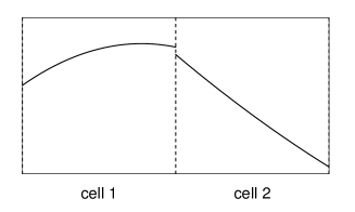
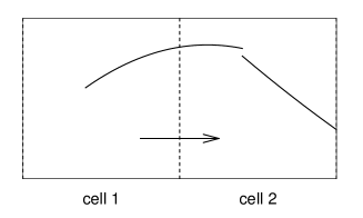
Figure 2: Illustration of the semi-Lagrangian discontinuous Galerkin approximation in a single space dimension. The discontinuous piecewise polynomial approximation is translated in space and then projected back to the finite dimensional subspace of piecewise polynomial functions.

In order to implement the numerical scheme, we still have to choose a basis for the space of cell-wise polynomials of degree $\ell$. This then also determines the degrees of freedom stored in computer memory. Our implementation is based on the Lagrange basis at the Gauss–Legendre quadrature nodes. Thus, the degrees of freedom correspond to the value of the function at the Gauss–Legendre nodes in each cell. However, in certain situations, it is more convenient to express the piecewise polynomial function in the Legendre basis. Thus, we can write (for an $L^{2}$ function $u$)

$$u(x)\approx Pu(x)=\sum_{i=0}^{N-1}\sum_{j=0}^{\ell}u_{ij}p_{ij}(x),$$

where $p_{ij}$ is the (appropriately scaled) $j$th Legendre polynomials in the $i$th cell and $N$ is the number of cells. The coefficients in the expansion are then given by

$$u_{ij}=\int u(x)p_{ij}(x)\,\mathrm{d}x.$$

Since the Legendre polynomials form an orthogonal basis, we have

$$\int u(x)\,\mathrm{d}x=\sum_{i}u_{i0}=\int Pu(x)\,\mathrm{d}x$$

and thus we follow that the numerical scheme is charge conservative.

Before proceeding, let us make two remarks. First, the semi-Lagrangian discontinuous Galerkin method is fully explicit. That is, no linear system of equations has to be solved. Second, the order of the space discretization is $p+1$ and thus we can easily construct numerical schemes of arbitrary order. Note, however, that the degrees of freedom are directly proportional to the order of the method. We will revisit this issue in some detail in section 4.

Up to this point we have described the numerical schemes used to solve the Vlasov equation. However, what we have not discussed so far is how to solve Poisson’s equation in order to determine the electric field from the charge density. Since the electric field is usually a smooth function, we can use the fast Fourier transformation (FFT). This is straightforward for the cubic spline interpolation as the degrees of freedom already reside on an equidistant grid. However, for the discontinuous Galerkin approach the degrees of freedom are located at the Gauss–Legendre quadrature nodes and thus have to be transferred to an equidistant grid before an FFT algorithm can be applied. In our implementation we simply evaluate the piecewise polynomial in order to obtain an equidistant grid. For example, for a piecewise linear approximation and the cell $[x_{i-1/2},x_{i-1/2}+h]$ we evaluate the approximant at $x_{i-1/2}+\tfrac{1}{3}h$ and $x_{i-1/2}+\tfrac{2}{3}h$ which yields an equidistant grid. In addition, once the electric field has been computed it has to be transferred back from an equidistant grid to the Gauss–Legendre quadrature nodes. In our implementation we use a polynomial interpolation that is of the same order as the discontinuous Galerkin scheme. Since this part of the algorithm takes place in a lower dimensional space, we could, in principle, use a more elaborate interpolation scheme without significantly increasing the computational cost. In sections 3 and 4 we will further investigate the effect of this interpolation on the conservation properties of the numerical scheme.

3 Conservation

The purpose of this section is to analyze the conservation properties from a theoretical point of view. The conserved variables (for the continuous system) which we will consider here are: charge, $L^{1}$ norm of the density function, current, energy, entropy, and the $L^{2}$ norm of the density function. We will first consider the error that is made due to the time discretization (the splitting approach outlined in the introduction) and then consider the error made due to the discontinuous Galerkin or the cubic spline interpolation that are used to discretize space. An overview of the properties of each scheme is given in table 1.

conserved var.	splitting	dG	spline	remarks
charge	yes	yes	yes
current	yes	$\text{yes}^{\dagger}$	$\text{yes}^{\dagger}$	additional error term for $\ell=0$
energy	no	no	no	additional error term for $\ell=0$, $\ell=1$
entropy	yes	no	no
$L^{1}$	yes	$\text{no}^{\ast}$	no
$L^{2}$	yes	no	no

Table 1: This table provides an overview of the conserved quantities for the splitting approach in time and the two space discretization strategies. The superscript $\dagger$ means the the conservation is only true up to an error made in the computation of the electric field. The superscript $\ast$ emphasizes that positivity preserving semi-Lagrangian discontinuous Galerkin schemes have been developed that do preserve the $L^{1}$ norm as well as the mass. The degree of the polynomial in each cell (for the sldg scheme) is denoted by $\ell$ and the corresponding numerical method is consistent of order $\ell+1$ in space.

3.1 Time discretization

Charge and $L^{p}$ norms

Since we can write both parts of the splitting as a translation along a coordinate axis in phase space, we immediately conclude that the splitting conserves the mass as well as all $L^{p}$ norms.

Current

More interesting is the conservation of the (total) current. The current is defined by the following relation

$$j=\int vg(x,v)\,\mathrm{d}(x,v).$$

For the first part of the splitting (see (3)) we immediately have

$$\int vg(x-vt,v)\,\mathrm{d}(x,v)=\int vg(x,v)\,\mathrm{d}(x,v)$$

which is the desired conservation of the current. For the second part of the splitting (see (4)) we get

$$\int vg(x,v-E(x)t)\,\mathrm{d}(x,v) =\int(v+E(x)t)g(x,v)\,\mathrm{d}(x,v)$$

$$=\int vg(x,v)\,\mathrm{d}(x,v)+t\int E(x)\rho(x)\,\mathrm{d}x.$$

Then from

$$\int E\rho\,\mathrm{d}x =\int E(\nabla\cdot E)\,\mathrm{d}x$$

$$=\int E(\nabla\cdot E)+\tfrac{1}{2}\nabla E^{2}\,\mathrm{d}x$$

$$=-\int(\nabla\times E)\times E\,\mathrm{d}x$$

$$=0$$

the conservation of the current follows immediately. Note that we have assumed here that the electric field is computed exactly and that it is curl free. Both of these assumptions are obviously satisfied if we neglect the space discretization. However, we will have to consider these assumptions in more detail in the next section.

Energy

The total energy is given by

$$E=\int\tfrac{1}{2}v^{2}g(x,v)\,\mathrm{d}(x,v)+\int\tfrac{1}{2}E^{2}(x)\,\mathrm{d}x,$$

where the first term represents the kinetic energy and the second term represents the energy stored in the electric field. The first part of the splitting conserves the kinetic energy

$$\int v^{2}g(x-tv,v)\,\mathrm{d}(x,v)=\int v^{2}g(x,v)\,\mathrm{d}(x,v)$$

and the second part of the splitting conserves the electric energy (since the charge density is not changed). However, in both cases the reverse statement is not true. Thus, the second part of the splitting does not conserve the electric energy and the first part of the splitting does not conserve the kinetic energy. Most importantly, the complete splitting procedure does not conserve the total energy.

This is to be expected. The splitting scheme considered here is a Hamiltonian splitting (see, for example, Casas et al. (2015)). Such numerical methods have been studied extensively in the case of ordinary differential equations (see, for example, Hairer et al. (2006)). While these numerical methods do not conserve energy, they show excellent long time properties with respect to energy conservation. The results for ordinary differential equations can not be directly transferred to the present case. The hope is, however, that similar long time properties can also be observed for the Vlasov–Poisson equation.

Entropy

The entropy is defined as

$$S=-\int g\log g\,\mathrm{d}(x,v).$$ (5)

For physically reasonable initial values (i.e. $g\geq 0$) the entropy is well defined and conserved by the continuous system. Entropy is maximized for a density function which has equal probability for each point in phase space. Since diffusive systems naturally tend to this limit, we use entropy as a measure of the amount of diffusion that is introduced by the numerical scheme.

To analyze the splitting scheme, we define $f(t,x,v)=g(x-tv,v)$. Then, for the first part of the splitting algorithm, we have

$$\partial_{t}\int f\log f\,\mathrm{d}(x,v) =-\int(\log f)\nabla\cdot(vf)\,\mathrm{d}(x,v)-\int\nabla\cdot(vf)\,\mathrm{d}(x,v).$$

Integration by parts yields

$$\int(\log f)\nabla\cdot(vf)\,\mathrm{d}(x,v)=-\int fv\cdot\nabla\log f\,\mathrm{d}(x,v)=-\int\nabla\cdot(vf)\,\mathrm{d}(x,v)=0$$

and thus entropy is conserved for the first part of the splitting algorithm.

Now, for the second step in the splitting algorithm we define $f(t,x,v)=g(x,v-tE(x))$ and get

$$\partial_{t}\int f\log f\,\mathrm{d}(x,v)=-\int(\log f)\nabla_{v}\cdot(Ef)\,\mathrm{d}(x,v)-\int\nabla_{v}\cdot(Ef)\,\mathrm{d}(x,v)=0$$

which shows that entropy is conserved for the splitting scheme.

3.2 Space discretization

Charge and $L^{1}$ norm

The discontinuous Galerkin method is charge conservative (see section 2). The same is true for the spline interpolation. However, both numerical methods can produce negative values. This, in principle, is not an issue for the algorithm considered here. The only difficulty that might arise is the physical interpretation of the resulting particle density function. Note, however, that as long as the magnitude of the negative values are smaller than the accuracy required, this issue is essentially void. However, an interesting aspect is that with respect to conservation of the $L^{1}$ norm we can formulate the following result.

Theorem 1

A numerical algorithm that produces negative values and is mass conservative can not conserve the $L^{1}$ norm.

Proof 3.2.

We assume that the initial value $f(0,x,v)$ is non-negative. Then

$$\int|f(0,x,v)|\,\mathrm{d}(x,v)=\int f(0,x,v)\,\mathrm{d}(x,v)=\int f(t,x,v)\,\mathrm{d}(x,v)\leq\int|f(t,x,v)|\,\mathrm{d}(x,v).$$

The inequality becomes strict if the particle density function $f(t,x,v)$ is negative. In this case the $L^{1}$ norm is not conserved which is the desired result.

The above result shows that conservation of $L^{1}$ norm can be used as a measure of positivity preservation. Both the discontinuous Galerkin scheme and the method based on cubic splines, at least in their most basic formulation, can yield negative values. Thus, they do not preserve the $L^{1}$ norm. For the discontinuous Galerkin scheme (mass conservative) limiters are available that restrict the density function in such a manner that negative values are avoided (Rossmanith & Seal, 2011; Qiu & Shu, 2011). The resulting schemes are then both mass and $L^{1}$ conservative. One should note, however, that while the proposed positivity limiters can be applied locally, associated to them is a certain computational cost. What is even more important is that these procedure might degrade the performance of the scheme with respect to the other conserved quantities. For example, the limiters suggested in Rossmanith & Seal (2011) and Qiu & Shu (2011) operate by shifting and scaling the output from the translation in order to avoid negative values. However, in order to conserve mass, a positive shift must result in a compression of the polynomial function which in turn introduces additional diffusion into the numerical scheme.

On the other hand, for the cubic spline interpolation implementing a positivity limiter is significantly more complicated. Nevertheless, a number of limiters have been suggested in the literature (Zerroukat et al., 2005, 2006; Crouseilles et al., 2010). It has been well established in this case that adding positivity limiters to the numerical scheme degrades the conservation of the other invariants.

We will not focus on positivity limiters in this paper. However, we will investigate the appearance of negative values in some detail in section 4. In fact, the numerical results obtained seem to suggest that even without such modifications we observe good long time behavior for the semi-Lagrangian discontinuous Galerkin scheme.

Current

In the following, we will use $g(x,v)=(Pf(\cdot-vt,v))(x)$. From section 2 we know that both the discontinuous Galerkin and the cubic spline based scheme are mass conservative and thus

$$\int g(x,v)\,\mathrm{d}x=\int f(x-vt,v)\,\mathrm{d}x.$$

For the first part of the splitting algorithm we thus have

$$\int vg(x,v)\,\mathrm{d}(x,v)=\int v\left(\int g(x,v)\,\mathrm{d}x\right)\mathrm{d}v=\int v\left(\int f(x-vt,v)\,\mathrm{d}x\right)\mathrm{d}v=\int vf(x,v)\mathrm{\,d}(x,y),$$

which implies that the current is conserved for that step of the algorithm.

The situation is more involved for the second part of the splitting algorithm. This is due to the fact that the translation is now in the velocity direction. We will thus consider the two numerical schemes separately, starting with the discontinuous Galerkin method. To simplify the notation let us define $g(x,v)=(Pf(x,\cdot-tE(x)))(v)$. Expanding $v$ in the Legendre basis (in a given cell) yields

$$v=v_{0}p_{0}+v_{1}p_{1}(v),$$

where $p_{k}$ is the $k$th Legendre polynomial in the corresponding cell. Thus, we get

$$\int vg(x,v)\,\mathrm{d}(x,v) =\int\left(\int(v_{0}p_{0}+v_{1}p_{1}(v))g(x,v)\,\mathrm{d}v\right)\mathrm{d}x$$

$$=\int\left[v_{0}p_{0}\int f(x,v-tE(x))\,\mathrm{d}v+v_{1}\int p_{1}(v)g(x,v)\,\mathrm{d}v\right]\,\mathrm{d}x.$$

Now, since we can expand the function $v\mapsto g(x,v)$ into

$$g(x,v)=\sum_{k=0}^{\ell}g_{k}(x)p_{k}(v)$$ (6)

we have (for $\ell\geq 1$)

$$\int p_{1}(v)g(x,v)\,\mathrm{d}v=g_{1}(x)=\int p_{1}(v)f(x,v-tE(x))\,\mathrm{d}x$$

and thus

$$\int vg(x,v)\,\mathrm{d}(x,v)=\int vf(x,v-tE(x))\,\mathrm{d}(x,v).$$

The only remaining issue is that we do not use the exact electric field in our computation but replace it by a numerical approximation. In principle, we can use an FFT based approach to compute the electric field up to machine precision. However, the discontinuous Galerkin approach requires an interpolation procedure in order to transfer the data from and to the equidistant grid required to compute the FFT. This transformation is not exact up to machine precision and does introduce an error in the total current. We will investigate this issue in section 4.

Now, let us consider the semi Lagrangian method based on the cubic spline interpolation. That the first part of the splitting algorithm conserves the current is an immediate consequence of the fact that that scheme is mass conservative. For the second part of the splitting algorithm we have

$$\sum_{j}v_{j}(Pf(x,\cdot-tE(x)))(v_{j})=\sum_{j}v_{j}f(x,v_{j}-tE(x))$$

since the projection does not change the value of the spline at the grid points. Thus, we follow that the cubic spline interpolation preserves the current under the assumption that the electric field is determined up to machine precision. Note that satisfying this assumption is easier in the case of the spline based semi-Lagrangian scheme, as the degrees of freedom already reside on an uniform grid and can thus be directly fed into an FFT based Poisson solver.

Energy

We have seen in the previous section that the splitting scheme does not conserve the total energy. Thus, the question posed in this section is if the space discretization introduces an additional error source.

First, let us consider the discontinuous Galerkin scheme. For the first part of the splitting we define $g(x,v)=(Pf(\cdot-vt,x))(x)$ and obtain (using conservation of mass)

$$\int v^{2}g(x,v)\,\mathrm{d}(x,v)=\int v^{2}\left(\int g(x,v)\,\mathrm{d}x\right)\,\mathrm{d}v=\int v^{2}\left(\int f(x-vt,v)\,\mathrm{d}x\right)\,\mathrm{d}v.$$

Now, we can rewrite the integrals on the right-hand side as follows

$$\int v^{2}\left(\int f(x-vt,v)\,\mathrm{d}x\right)\,\mathrm{d}v=\int v^{2}f(x-vt,v)\,\mathrm{d}(x,v)$$

which shows that the kinetic energy is preserved. On the other hand, the first splitting step does not conserve the electric energy. Thus, we consider here only if the space discretization modifies the electric energy that we obtain from the time integrator. This is indeed the case as in general

$$\int f(x-vt,v)\,\mathrm{d}v\neq\int g(x,v)\,\mathrm{d}v$$

which shows that the space discretization modifies the charge density and thus the electric field. Therefore, the space discretization introduces an additional error source in the electric energy.

For the second part of the splitting we define $g(x,v)=(Pf(x,\cdot-tE(x)))(v)$ and obtain in each cell (by using (6))

$$\int v^{2}g(x,v)\,\mathrm{d}(x,v) =\int\left(\sum_{k=0}^{2}\sum_{j=0}^{\ell}v_{k}g_{j}(x)\int p_{k}(v)p_{j}(v)\,\mathrm{d}v\right)\,\mathrm{d}x$$

$$=\int\sum_{k=0}^{\min(2,\ell)}v_{k}g_{k}\,\mathrm{d}x$$

$$=\int\left(\sum_{k=0}^{\min(2,\ell)}v_{k}\int p_{k}(v)f(x,v-tE(x))\,\mathrm{d}v\right)\,\mathrm{d}x$$

$$=\int v^{2}f(x,v-tE(x))\,\mathrm{d}(x,v).$$

The last equality only holds for $\ell\geq 2$ and shows that in this case no additional error in the kinetic energy is introduced by the space discretization. Now, the second part of the splitting does not change the charge density and thus the electric energy remains invariant. Since

$$\rho(x)=\int f(x,v-tE(x))\,\mathrm{d}v=\int g(x,v)\,\mathrm{d}v,$$

the same property holds true for the discontinuous Galerkin approximation and thus the electric energy is conserved during that step (i.e. no additional error is introduced by the space discretization).

Most of the results obtained for the semi-Lagrangian discontinuous Galerkin scheme can be transferred immediately to the case of spline interpolation. Since the projection on the spline subspace does not change the value of the approximant at the grid points, we have

$$\sum_{j}v_{j}^{2}g(x,v_{j})=\sum_{j}v_{j}^{2}f(x,v_{j}-tE(x))$$

and thus the second part of the splitting does not introduce an additional source of error (independent of the order of the underlying polynomials).

Entropy and $L^{2}$ norm

For both the semi-Lagrangian discontinuous Galerkin scheme and the cubic spline based scheme the entropy and the $L^{2}$ norm are not conserved; even though both are conserved by the splitting algorithm. We will evaluate the relative error made in the conservation of these quantities in the next section. However, for now, we will discuss one additional issue not directly related to conservation.

In the Vlasov–Poisson equations no diffusion mechanism is included. Thus, the $L^{2}$ norm and the entropy are conserved for the continuous model. However, once diffusion is added, the $L^{2}$ norm will decrease in time. This is due to the fact that diffusion decreases the variance of the density function $f$ and we can write $\|f\|_{2}^{2}=1+\text{Var}(f)$. In addition, diffusion increases the entropy (which is a measure of the disorder of a system). The latter property is, of course, just a statement of the second law of thermodynamics. Thus, the decrease in the $L^{2}$ norm and the increase in entropy can be considered as a measure of the amount of diffusion in a given physical system. In our case they are used to quantify the amount of diffusion that a numerical scheme (wrongly) introduces. This point is interesting because in the numerical simulations conducted in the next section we observe that the semi-Lagrangian discontinuous Galerkin scheme always decreases/increases the $L^{2}$ norm/entropy while the spline based approach shows an oscillating behavior for some problems. Thus, the spline based semi-Lagrangian method cannot be considered as the exact solution of a perturbed physical system (as no such system would be allowed to decrease the entropy; a consequence of the second law of thermodynamics).

Analytically, we can show that the $L^{2}$ norm decreases in time for the semi-Lagrangian discontinuous Galerkin scheme.

Theorem 3.3.

The $L^{2}$ norm is a decreasing function of time for the semi-Lagrangian discontinuous Galerkin scheme.

Proof 3.4.

Due to the structure of the Vlasov–Poisson equation it is sufficient to consider a one-dimensional advection problems. Thus, we consider a translated function $g(x)$ which is piecewise polynomial and thus lies in $L^{2}$. We can then find a Legendre series

$$\sum_{k=0}^{\infty}g_{k}p_{k}(x)$$

which converges in the $L^{2}$ norm to $g$ (Pollard, 1972). Now, we have

$$\|Pg\|_{2}^{2}-\|g\|_{2}^{2}=\sum_{k=0}^{\ell}g_{k}^{2}-\sum_{k=0}^{\infty}g_{k}^{2}\leq 0$$

which implies that the $L^{2}$ norm decreases in each time step.

Based on an extensive numerical investigation, we conjecture that a similar result holds true for the entropy. In fact, for piecewise constant polynomials this immediately follows from the convexity of the logarithm and for piecewise linear polynomials a similar (although more tedious) argument can be given. However, we were not able to prove the corresponding result for piecewise polynomials of arbitrary degree.

There is one additional complication in case of the entropy. As the numerical scheme can generate negative values, the entropy as given by (5) is not even defined. Since we interpret negative values as zero particle density, we use

$$S=-\int\max(g,0)\log g\,\mathrm{d}(x,v)$$

instead. Of course, using this formula can still result in a decrease of entropy. However, we will see in the next section that this issue only plays a negligible role in the numerical simulations.

4 Numerical results

Before we discuss the results of the medium and long time simulations, which are the main focus of this paper, let us start by establishing some baseline results for relatively small final times in case of the linear Landau damping (see section 4.4 for more details on the parameters used). In this case we have computed the error for both the electric field $E$ and the particle distribution $f$ at final time $T=12.5$ and $T=100$. The corresponding results are shown in Figure 3.

For final time $T=12.5$ we observe convergence of the discontinuous Galerkin schemes with the expected order. In addition, the sixth order scheme is always superior to the fourth order scheme which in turn is superior to the second order scheme. The comparison with the cubic spline interpolation is a bit more nuanced. In particular, we see a clear advantage of the fourth and sixth order discontinuous Galerkin methods for the error in the electric field. On the other hand, with respect to the error in the distribution function the cubic spline interpolation performs best (except for very stringent accuracy requirements).

For the final time $T=100$ the analytic solution is almost identical to zero. However, numerical methods have significant difficulties due to the recurrence effect (see section 4.4 for more details). We can see this in the numerical results very clearly as initially no convergence is observed (up to $128$ degrees of freedom). Since the recurrence effect depends mostly on the grid spacing, the spline interpolation performs best in this case (this is due to the fact that an equidistant grid minimizes the grid spacing). We also note that for low tolerances the second order dG method performs better than the higher order variants if one is only interested in resolving the error in the electric field. Some of this conclusions have been pointed our in earlier work. For example, it was observed in Crouseilles et al. (2011b); Einkemmer & Ostermann (2014b) that higher order discontinuous Galerkin methods only have a weak influence on the recurrence effect.

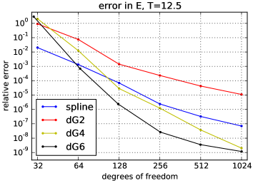
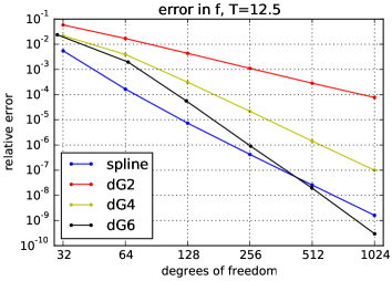
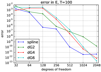
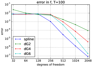
Figure 3: The error for linear Landau damping in the electric field $E$ and the particle distribution $f$ is shown as a function of the degrees of freedom (per dimension) for the second, fourth, and sixth order discontinuous Galerkin method and the cubic spline interpolation. The results for final time $T=12.5$ are shown in the top row and the results for final time $T=100$ are shown in the bottom row.

The remainder of this section is divided into two parts. In the first part we mainly discuss the properties of the semi-Lagrangian discontinuous Galerkin scheme and compare its efficiency to the cubic spline interpolation. We will consider both classic test problems (linear and nonlinear Landau damping, bump-on-tail instability) and a somewhat less well known test problem (expansion of a plasma blob, plasma echo). In the second part we will consider the long time behavior of the semi-Lagrangian discontinuous Galerkin scheme. These simulations are conducted with the highly parallel implementation described in Einkemmer (2016b).

Since one of our goals is to compare the discontinuous Galerkin scheme with the cubic spline interpolation, a measure of the cost of a given numerical scheme has to be established. In a sequential implementation both computational efficiency as well as memory consumption is a possible choice. However, comparing arithmetic operations on a modern (vectorized and multi-core) CPU requires a very delicate analysis that depends on both algorithmic and implementation details (for example, taking into account how the linear system is solved in the cubic spline interpolation or whether such a scheme could be vectorized). In addition, on a distributed memory system (i.e. on a cluster), especially for the cubic spline interpolation, further problems occur due to the all-to-all communication required in solving the linear system. Some remedies have been proposed in Crouseilles et al. (2009a). However, these usually change the numerical scheme in a non-trivial way (which might also have a detrimental effect on the conserved quantities). In fact, this problem is one of the major motivations why we consider the discontinuous Galerkin approach.

In the present study we will exclusively use the number of degrees of freedom, i.e. the memory consumed, as the measure of efficiency. This is reasonable because for higher dimensional simulations the amount of memory consumed is often the most important criterium for Vlasov simulations. But perhaps even more important is the fact that such algorithms are bandwidth limited on all modern architectures. Consequently, how many bytes have to be transferred to and from the CPU determines the run time of the algorithm. We have implemented our discontinuous Galerkin approach on a dual socket Intel Xeon E5-2630 v3 workstation with a (theoretical) memory bandwidth of 59 GB/s. For the second order implementation (dG2)/fourth order (dG4) implementation we achieve approximately $94$%/ $89$% of the theoretically possible performance on that machine. That means that for the advection step with contiguous memory access we require approximately $0.3$ ns per degree of freedom. Let us also note that this means, in particular, that no spline implementation is able to outperform our algorithm by more than $10$% (in all likelihood, even an optimized spline implementation will probably be significantly slower; due to the fact that extra data structures are required to store the spline coefficients). We further note that the discontinuous Galerkin method has been implemented on graphic processing units (GPUs) and the Intel Xeon Phi. The corresponding performance measurements, which show a significant speedup on both of these architectures, are given in Einkemmer (2016a).

In the remainder of this section we will conduct two-dimensional simulations of the Vlasov–Poisson equations using $128$ degrees of freedom in each dimension (the coarse problem) and $512$ degrees of freedom in each dimension (the fine problem).

4.1 Nonlinear Landau damping

We begin with the classic problem of nonlinear Landau damping. The initial value

$$f(0,x,v)=\frac{1}{\sqrt{2\pi}}\mathrm{e}^{-v^{2}/2}(1+\alpha\cos kx)$$

is posed on the domain $[0,4\pi]\times[-6,6]$ with $k=\tfrac{1}{2}$ and $\alpha=\tfrac{1}{2}$. Periodic boundary conditions are imposed in both the $x$- and the $v$-direction. A large body of physics literature has been devoted to this problem and a number of numerical simulations have been conducted (see, for example, Brunetti et al. (2000) and Manfredi (1997)). As such the behavior, at least for moderate times, is fairly well understood. Initially we observe a decay in the electric energy (the Landau damping phenomenon) that after some time stabilizes and gives way to oscillations of the electric energy. The nonlinear Landau damping is numerically challenging because even though the initial value is perfectly smooth, small scale structures (so-called filaments) develop in the two-dimensional phase space as the system evolves in time. Thus, in order to integrate the system up to a given precision an extremely high resolution in velocity space is needed. However, what we are interested in is to what extend a relatively coarse discretization can give qualitatively correct results.

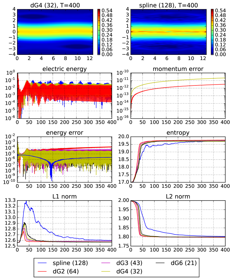
Figure 4: This figure shows the particle density $f$ at $T=400$ and the time evolution of the electric energy for the nonlinear Landau damping problem. In addition, the error in the current, energy, entropy, $L^{1}$ norm, and $L^{2}$ norm are shown. For all numerical schemes $128$ degrees of freedom are employed per space dimension. The order of the discontinuous Galerkin (dG) method is indicated and the number of cells are given in parenthesis.

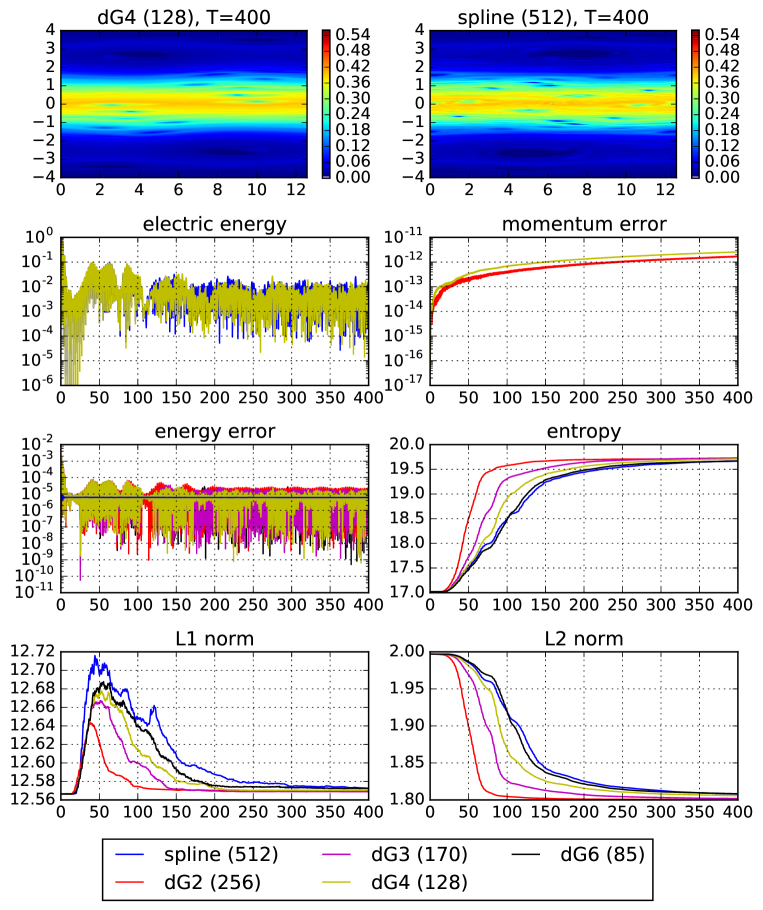
Figure 5: This figure shows the particle density $f$ at $T=400$ and the time evolution of the electric energy for the nonlinear Landau damping problem. In addition, the error in the current, energy, entropy $L^{1}$, and $L^{2}$ norm are shown. For all numerical schemes $512$ degrees of freedom are employed per space dimension. The order of the discontinuous Galerkin (dG) method is indicated and the number of cells are given in parenthesis.

The numerical simulations for the cubic spline and the discontinuous Galerkin approach are given in figure 4 (for the coarse discretization) and in figure 5 (for the fine discretization). We observe that for the discontinuous Galerkin method the error in the current is close to machine precision (even though this quantity is not exactly conserved). The cubic spline interpolation has an advantage with respect to the energy error (which, however, is quite accurately conserved for this test problem). We also observe a distinct difference between the second order method ($p=1$) and the higher order methods with respect to energy conservation (as predicted by the results derived in section 3).

On the other hand, the discontinuous Galerkin scheme has an advantage with respect to the $L^{1}$ norm (an error of 5% vs 1-2% for the coarse problem). Thus, the discontinuous Galerkin scheme produces fewer negative values. If we consider the qualitative features of the numerical solution we might be tempted to conclude that the spline interpolation reproduces more clearly the features of the exact solution. However, upon closer inspection of the results for the fine discretization (where the maximal amplitude is significantly reduced for the spline interpolation) and taking into account the error in the $L^{1}$ norm, we conclude that in fact the spline interpolation produces significant overshoot into the numerical simulation.

Let us also discuss the effect of the order of the discontinuous Galerkin approximation. For the coarse problem the order does only play a minor role (although energy conservation is better once we consider a numerical scheme with piecewise polynomials of degree $2$ or above). Other than that the performance of the numerical scheme is almost independent of the order.

4.2 Bump-on-tail instability

The second problem we consider is the so-called bump-on-tail instability. In this case we prescribe the initial value

$$f(0,x,v)=\frac{1}{\sqrt{2\pi}}\left(\alpha\mathrm{e}^{-v^{2}/2}+\beta\mathrm{e}^{-4(v-2.5)^{2}}(1+\gamma\cos x)\right)$$

on the domain $[0,4\pi]\times[-6,6]$ and with $\alpha=0.8$, $\beta=0.2$ and $\gamma=0.1$. Periodic boundary conditions in both the $x$- and the $v$-direction are imposed. Thus, we have a stationary thermal plasma in which $80$% of the mass is concentrated. In addition, a smaller beam with average velocity $v=2.5$ penetrates the stationary plasma. This configuration is an equilibrium of the Vlasov–Poisson equation. However, due to the perturbation that is added, a traveling vortex appears in phase space. The bump-on-tail instability shows a quiet phase that is succeeded by the relative rapid development of the vortex which then remains stable for a long time. Since the bump-on-tail instability exhibits chaotic behavior the onset of the vortex might be different for different numerical schemes (even for relatively fine discretizations).

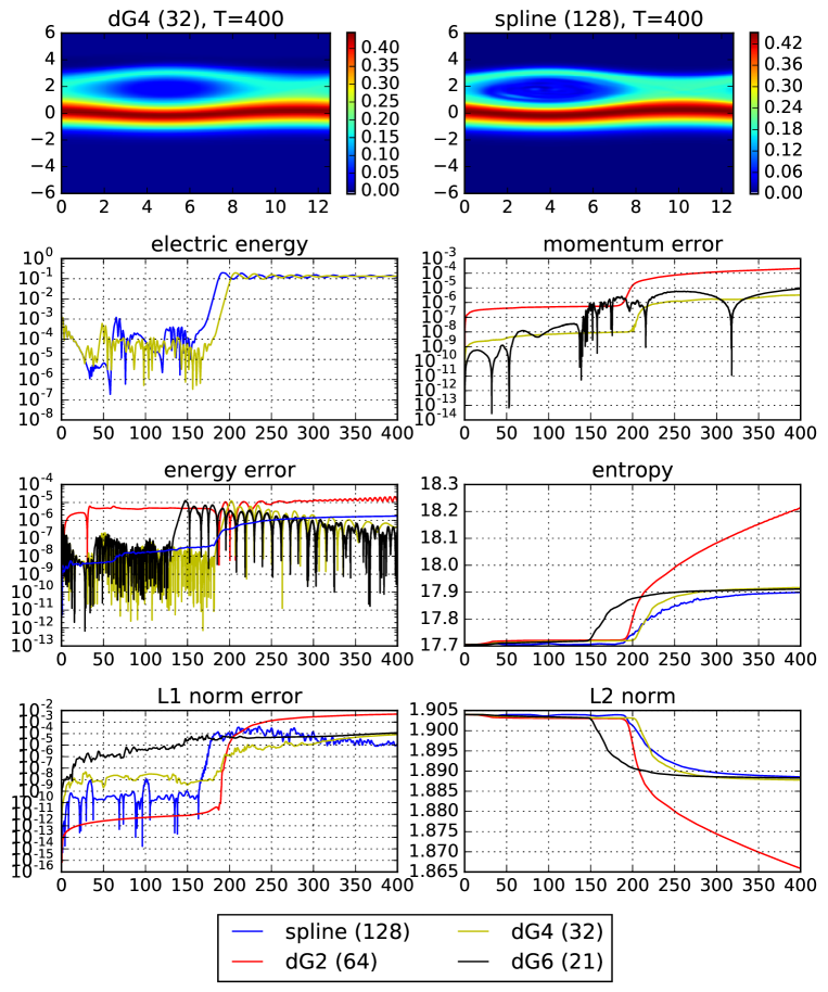
Figure 6: This figure shows the particle density $f$ at $T=400$ and the time evolution of the electric energy for the bump-on-tail instability. In addition, the error in the current, energy, entropy, $L^{1}$ norm, and $L^{2}$ norm are shown. For all numerical schemes $128$ degrees of freedom are employed per space dimension. The order of the discontinuous Galerkin (dG) method is indicated and the number of cells are given in parenthesis.

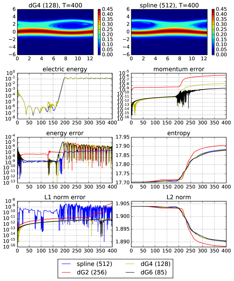
Figure 7: This figure shows the particle density $f$ at $T=400$ and the time evolution of the electric energy for the bump-on-tail instability. In addition, the error in the current, energy, entropy $L^{1}$, and $L^{2}$ norm are shown. For all numerical schemes $512$ degrees of freedom are employed per space dimension. The order of the discontinuous Galerkin (dG) method is indicated and the number of cells are given in parenthesis.

The numerical simulations for the cubic spline and the discontinuous Galerkin approach are given in figure 6 (for the coarse discretization) and in figure 7 (for the fine discretization). The current in case of the discontinuous Galerkin scheme is only conserved up to $10^{-5}$ which clearly confirms the behavior discussed in section 3. However, this fact does not seem to diminish the overall performance of the numerical scheme. For the higher order discontinuous Galerkin scheme and for the cubic spline interpolation all the remaining conserved quantities show a similar behavior. The exception being the second order discontinuous Galerkin scheme which exhibits significantly worse performance across the board (contrary to the results obtained in the previous section for the nonlinear Landau damping).

Let us remark that for both schemes the time evolution of the electric energy is almost indistinguishable from the finer space discretization once the instability has been saturated.

4.3 Expansion into a uniform ion background

In this section we consider the following initial value

$$f(0,x,v)=\frac{1}{2\pi}\mathrm{e}^{-v^{2}/2}\mathrm{e}^{-(x-2\pi)^{2}/2}$$

on the domain $[0,4\pi]\times[-6,6]$. As before, we impose periodic boundary conditions in both directions. This is the only test problem where the initial value is localized in space as well as in velocity. This problem can be interpreted as the expansion of an electron blob (in thermodynamic equilibrium) into a region of uniform ion density. This is a challenging problem because there is no physical mechanism that would hold the initial blob in place. Thus, each particle with a given velocity expands at its own speed which due to the periodicity of the problem yields a very irregular phase space distribution (similar to the nonlinear Landau damping). What sets this problem apart from the nonlinear Landau damping, however, is that the filamentation is driven by the free streaming part of the Vlasov equation and is not merely superimposed on top of a Maxwellian distribution in velocity space.

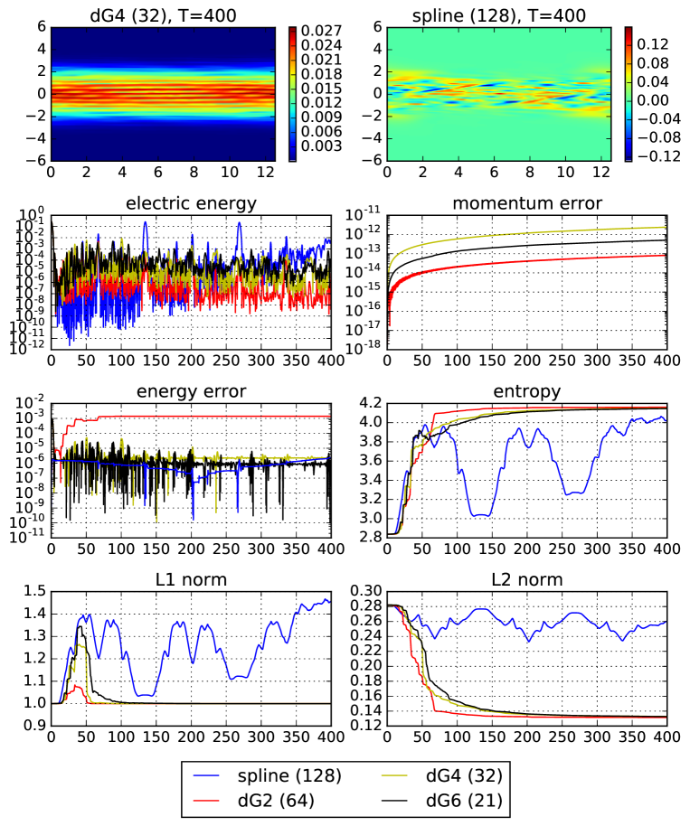
Figure 8: This figure shows the particle density $f$ at $T=400$ and the time evolution of the electric energy for the expansion into a uniform ion background. In addition, the error in the current, energy, entropy, $L^{1}$ norm, and $L^{2}$ norm are shown. For all numerical schemes $128$ degrees of freedom are employed per space dimension. The order of the discontinuous Galerkin (dG) method is indicated and the number of cells are given in parenthesis.

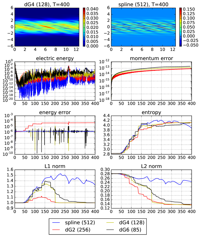
Figure 9: This figure shows the particle density $f$ at $T=400$ and the time evolution of the electric energy for the expansion into a uniform ion background. In addition, the error in the current, energy, entropy, $L^{1}$ norm, and $L^{2}$ norm are shown. For all numerical schemes $512$ degrees of freedom are employed per space dimension. The order of the discontinuous Galerkin (dG) method is indicated and the number of cells are given in parenthesis.

The numerical simulations for the cubic spline and the discontinuous Galerkin approach are given in figure 8 (for the coarse discretization) and in figure 9 (for the fine discretization). This problem seems to be especially challenging for the cubic spline interpolation. For the coarse discretization we observe an error of almost 50% in the $L^{1}$ norm, which renders any interpretation of the particle density function impossible. In addition, we observe two unphysical peaks in the electric energy.

On the other hand, none of these difficulties appear for the semi-Lagrangian discontinuous Galerkin scheme. With respect to the $L^{1}$ norm the second order dG method is most favorable although that method only conserves energy up to an accuracy of $10^{-3}$ (compared to $10^{-5}$ for the higher order methods). This favorable behavior is despite the fact that entropy conservation is somewhat better for the cubic spline approximation and the $L^{2}$ norm conservation is significantly better.

Let us continue to discuss the cubic spline interpolation. For this method the entropy and the $L^{2}$ norm show an oscillating behavior in time. Clearly this is a numerical artifact as has been discussed in section 3. None of these artifacts are present for the discontinuous Galerkin approach (as is expected based on the theoretical considerations in section 3).

4.4 Linear Landau damping

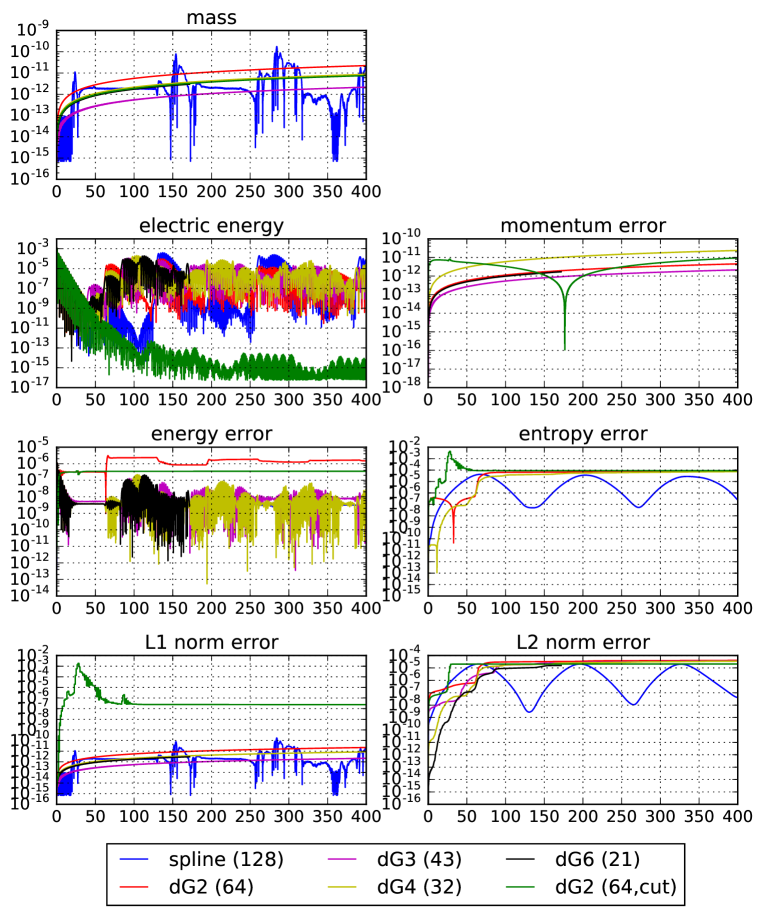
Figure 10: This figure shows the time evolution of the electric energy for the linear Landau damping. In addition, the error in the current, energy, entropy, $L^{1}$ norm, and $L^{2}$ norm are shown. For all numerical schemes $128$ degrees of freedom are employed per space dimension. The order of the discontinuous Galerkin (dG) method is indicated and the number of cells are given in parenthesis.

The linear Landau damping problem is just the strong Landau damping introduced earlier but with $\alpha$ chosen sufficiently small such that nonlinear effects are small. In this section we consider $\alpha=10^{-2}$. We have postponed this classic problem until now because in some sense the problem is very easy while in another sense it is very difficult. The numerical results for the coarse grid are shown in figure 10. All of the conserved quantities look very reasonable. In fact, $L^{1}$ is conserved up to machine precision and the $L^{2}$ norm and the entropy are conserved up to approximately an error of $10^{-5}$ (by far the lowest error among the problems considered so far). Nevertheless, the result of the numerical simulation is completely wrong (even considering a qualitative analysis). From analytical results it is well known that the electric energy decays exponentially as a function in time. What we observe for the numerical simulation, however, is that it oscillates. This is the so-called recurrence effect; a numerical artifact which implies that the number of grid points have to be chosen proportional to the final time in order to obtain reasonable results. This was already recognized in Cheng & Knorr (1976) and is the reason why despite the favorable conservation properties the linear Landau damping problem is difficult for any numerical scheme.

Unfortunately, a number of interesting problems in plasma physics (such as plasma echos; see Hou et al. (2011) or Galeotti & Califano (2005) for a good exposition) suffer from the recurrence effect. The problem can be overcome to some extend by filtering high frequencies in phase space (a technique referred to as filamentation filtration). In fact, a significant body of literature has been developed on this topic (Klimas & Farrell, 1994; Eliasson, 2002; Einkemmer & Ostermann, 2014a). However, even though, such methods can alleviate the problem to some extend, in many situations a fine velocity discretization is still required in order to resolve the interesting dynamics of the system. However, for such a fine discretization the conservation behavior is even better than for the relative coarse discretization used here.

At this point one might rightfully object that there is no guarantee that filamentation filtration will respect the invariants (even if they are conserved by the basic numerical scheme). Thus it seems prudent to investigate the effect of such a modification to the algorithm outlined in section 2. The results for the method introduced in Einkemmer & Ostermann (2014a) are shown in figure 10. There is some effect on the entropy and the $L^{1}$ norm which, however, are still conserved up to a accuracy of $10^{-2}$. However, despite the fact that we essentially remove high frequencies neither the mass nor any of the conserved quantities, except for the $L^{1}$ norm and the entropy, are adversely affected. This behavior is due to the fact that the magnitude of the high frequencies is very small and thus negative values appear. Since we cut off a couple of frequencies this averages out and leaves the mass intact (while affecting the $L^{1}$ norm).

Before proceeding, let us return to the question of how coarse a space discretization is sufficient in order to obtain reasonable results. To do this we consider a model of the plasma echo phenomenon. That is, we prescribe the initial value

$$f(0,x,v)=\frac{1}{\sqrt{2\pi}}\mathrm{e}^{-v^{2}/2}(1+\alpha\cos k_{1}x)$$

with $\alpha=10^{-3}$ and $k_{1}=12\pi/100$. This initial perturbation is damped away by Landau damping. Then at time $t=200$ we excite a second perturbation by adding

$$\frac{\alpha}{\sqrt{2\pi}}\mathrm{e}^{-v^{2}/2}\cos k_{2}x,$$

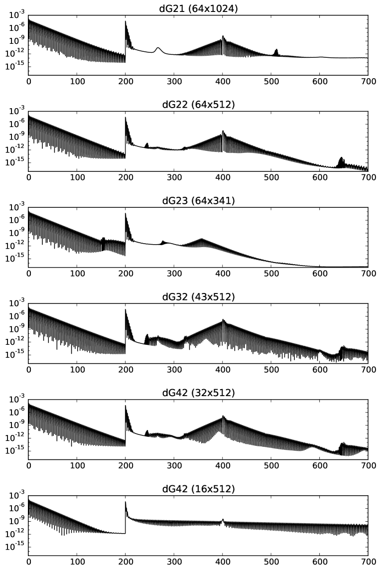
Figure 11: This figure shows the evolution of the electric energy for the plasma echo problem. The order of the discontinuous Galerkin (dG) method is indicated (dGab denotes a method with order a in the $x$-direction and order b in the $v$-direction) and the number of cells are given in parenthesis.

where $k_{2}=25\pi/100$, to the particle density function. This perturbation is also damped away by Landau damping. However, all the information is still stored in the particle density function and due to constructive interference an echo appears at $t=400$. In fact, multiple echoes can be observed. We will investigate how well the first echo is resolved by the semi-Lagrangian discontinuous Galerkin method. The numerical results are shown in figure 11. We note that in this situation increasing the order in the velocity direction, while keeping the number of degrees of freedom constant, significantly degrades the numerical solution. This is particular prominent for approximations of order three and higher, where the plasma echo is barely recognizable. In the spatial direction the results are comparable no matter what order is chosen. Note, however, that decreasing the number of degrees of freedom rapidly diminishes the numerical solution and the wave echo disappears. Thus, there is no point in studying the conservation properties at low resolution in the spatial direction as a certain number of cells are required even if one is only interested in resolving the first echo accurately.

4.5 Long time behavior (Nonlinear Landau)

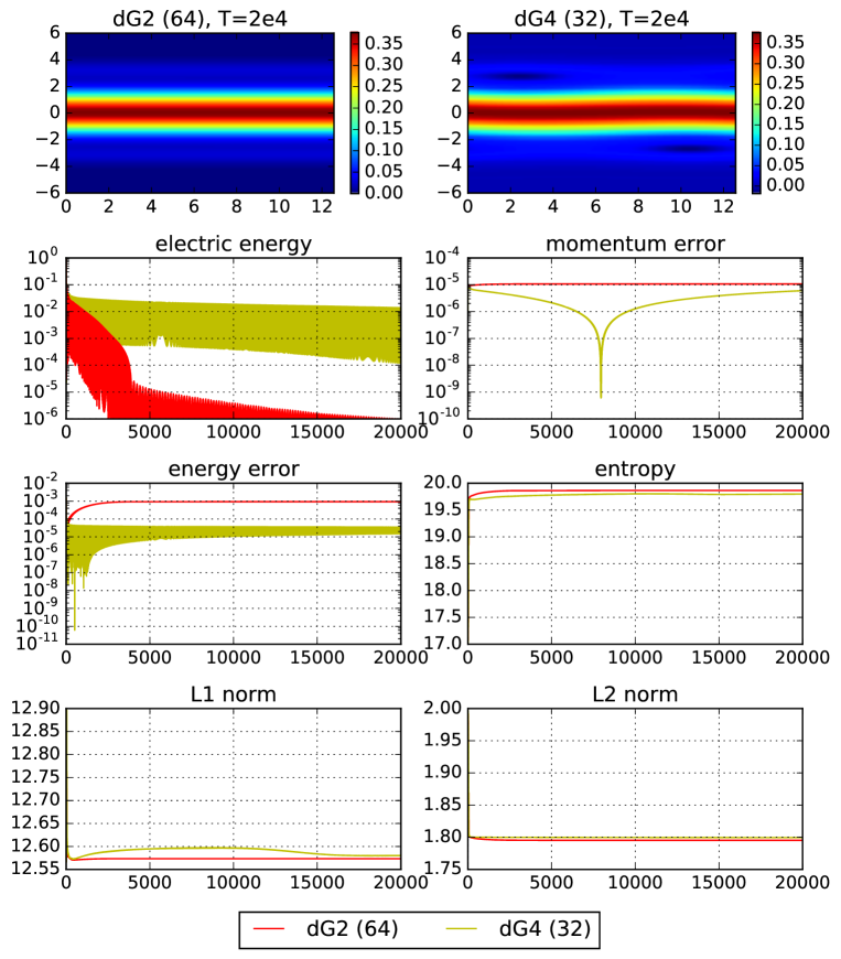
Figure 12: This figure shows the particle density $f$ at $T=2\cdot 10^{4}$ and the time evolution of the electric energy for the nonlinear Landau damping. In addition, the error in the current, energy, entropy, $L^{1}$ norm, and $L^{2}$ norm are shown. For all numerical schemes $128$ degrees of freedom are employed per space dimension. The order of the discontinuous Galerkin (dG) method is indicated and the number of cells are given in parenthesis.

We will now investigate the long time behavior for the semi-Lagrangian discontinuous Galerkin approach. To that end we integrate the Vlasov–Poisson equations until $T=2\cdot 10^{4}$ for the classic nonlinear Landau damping problem (as stated in section 4.1). The results are shown in figure 12 and compare the second order method with the fourth order method. Note that even though the conservation properties are quite similar (especially with respect to the $L^{2}$ norm and the entropy) the second order method produces qualitatively wrong results (the electric energy decays exponentially in time). Note that this rather different behavior is not expected based on the numerical results that were obtained up to final time $T=400$ (see section 4.1). On the other hand, the error in all the conserved quantities is stable over this time interval.

4.6 Long time behavior (bump-on-tail instability)

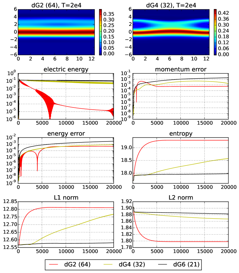
Figure 13: This figure shows the particle density $f$ at $T=2\cdot 10^{4}$ and the time evolution of the electric energy for the bump-on-tail instability. In addition, the error in the current, energy, entropy, $L^{1}$ norm, and $L^{2}$ norm are shown. For all numerical schemes $128$ degrees of freedom are employed per space dimension. The order of the discontinuous Galerkin (dG) method is indicated and the number of cells are given in parenthesis.

In this section we investigate the long time behavior of the semi-Lagrangian discontinuous Galerkin approach for the bump-on-tail instability by integrating the Vlasov–Poisson equation until $T=2\cdot 10^{4}$. The numerical results are shown in figure 13. Also in this case the second order method produces qualitatively wrong results. However, the conservation properties are also markedly worse for the second order method as compared to the fourth and sixth order methods. This is especially true for the entropy and $L^{2}$ norm (which measures diffusion) and we are thus not surprised that the second order method washes out the vortex in phase space. We also observe that the error in the current is quite large (conserved only up to approximately $10^{-2}$). This is true independent of the order of the method. However, this behavior is not detrimental to the other conserved quantities nor is it detrimental to the qualitative properties of the numerical solution.

4.7 Vortex merging in the bump-on-tail instability

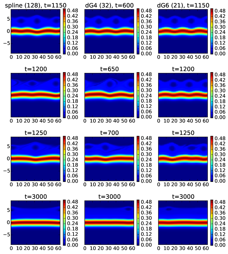
Figure 14: This figure shows the particle density $f$ at different times for the three vortex bump-on-tail instability. For all numerical schemes $128$ degrees of freedom are employed per space dimension. The order of the discontinuous Galerkin (dG) method is indicated and the number of cells are given in parenthesis.

In the previous section only one vortex appears in the bump-on-tail instability. However, for a certain regime of parameters multiple vortices can be observed in phase space. The difficulty for a numerical scheme is then to preserve these vortices as long as possible. However, most numerical schemes eventually lead to a secondary instability that results in the three vortices merging into a single one. In the following we will consider the problem from Crouseilles et al. (2011b) for which three vortices are observed in phase space. The numerical results are shown in figure 14. We note that vortex merging starts at approximately $t=650$ for the fourth order discontinuous Galerkin method and at approximately $t=1200$ for the spline interpolation. The sixth order discontinuous Galerkin schemes performs best in this test (vortex merging starts at approximately $t=1250$).

5 Conclusion

We conclude that the semi-Lagrangian discontinuous Galerkin scheme is certainly competitive compared to the cubic spline interpolation with respect to the invariants considered in this work. The latter seems to have a slight edge with respect to energy conservation (which, however, is always preserved up to an accuracy of $10^{-4}$ or better). On the other hand, the discontinuous Galerkin scheme outperforms the cubic spline interpolation with respect to the conservation of the $L^{1}$ norm (i.e.  positivity preservation) in all tests. This is particularly apparent in one test (the expansion into a uniform ion background) where the cubic spline interpolation results in over and undershoots that renders a physical interpretation of the particle density function impossible.

The second order variant of the discontinuous Galerkin scheme is usually quite diffusive. However, using the fourth or a higher order variant remedies this deficiency. Based on the conservation of the invariants the fourth order method is sufficient for most problems. However, for the bump-on-tail instability we observed a significant improvement, both in conservation as well as in long time behavior (onset of vortex merging), for the sixth order scheme. In general, the numerical results obtained emphasize the efficiency of high order methods (even though those methods reduce the number of cells present in the numerical simulation and this behavior is not expected based on the regularity of the solution). The exception to this rule is the plasma echo phenomenon (where increasing the order actually degrades the numerical solution).

In addition, we have seen that transferring the semi-Lagrangian scheme to an equidistant grid (in order to solve Poisson’s equation) does not result in any issues with respect to conservation of the invariants and long time behavior. The same is true for the filamentation filtration approach considered in this paper.

References

- Brunetti et al. (2000) Brunetti, M., Califano, F. & Pegoraro, F. 2000 Asymptotic evolution of nonlinear Landau damping. Phys. Rev. E 62 (3), 4109.
- Califano et al. (2006) Califano, F., Galeotti, L. & Mangeney, A. 2006 The Vlasov-Poisson model and the validity of a numerical approach. Phys. Plasmas 13 (8), 082102.
- Casas et al. (2015) Casas, F., Crouseilles, N., Faou, E. & Mehrenberger, M. 2015 High-order Hamiltonian splitting for Vlasov-Poisson equations. arXiv preprint, arXiv:1510.01841 .
- Cheng & Knorr (1976) Cheng, C. & Knorr, G. 1976 The integration of the Vlasov equation in configuration space. J. Comput. Phys. 22 (3), 330–351.
- Crouseilles et al. (2011a) Crouseilles, N., Faou, E. & Mehrenberger, M. 2011a High order Runge-Kutta-Nyström splitting methods for the Vlasov-Poisson equation. URL http://hal. inria. fr/inria-00633934 .
- Crouseilles et al. (2009a) Crouseilles, N., Latu, G. & Sonnendrücker, E. 2009a A parallel Vlasov solver based on local cubic spline interpolation on patches. J. Comput. Phys. 228 (5), 1429–1446.
- Crouseilles et al. (2010) Crouseilles, N., Mehrenberger, M. & Sonnendrücker, E. 2010 Conservative semi-Lagrangian schemes for Vlasov equations. J. Comput. Phys. 229 (6), 1927–1953.
- Crouseilles et al. (2011b) Crouseilles, N., Mehrenberger, M. & Vecil, F. 2011b Discontinuous Galerkin semi-Lagrangian method for Vlasov-Poisson. In ESAIM: Proceedings, , vol. 32, pp. 211–230. EDP Sciences.
- Crouseilles et al. (2009b) Crouseilles, N., Respaud, T. & Sonnendrücker, E. 2009b A forward semi-Lagrangian method for the numerical solution of the Vlasov equation. Comput. Phys. Commun. 180 (10), 1730–1745.
- E. Sonnendrücker (2011) E. Sonnendrücker 2011 Numerical methods for the Vlasov equation. http://icerm.brown.edu/html/programs/sp_f11/schedules/slides_workshop_1_tutorial/LectureNumericalVlasov.pdf.
- Einkemmer (2016a) Einkemmer, L. 2016a A mixed precision semi-Lagrangian algorithm and its performance on accelerators. In High Performance Computing and Simulation (HPCS), International Conference on.
- Einkemmer (2016b) Einkemmer, L. 2016b High performance computing aspects of a dimension independent semi-Lagrangian discontinuous Galerkin code. Comput. Phys. Commun. 202, 326–336.
- Einkemmer & Ostermann (2014a) Einkemmer, L. & Ostermann, A. 2014a A strategy to suppress recurrence in grid-based Vlasov solvers. EPJ B 68 (7), 1–7.
- Einkemmer & Ostermann (2014b) Einkemmer, L. & Ostermann, A. 2014b Convergence analysis of a discontinuous Galerkin/Strang splitting approximation for the Vlasov–Poisson equations. SIAM J. Numer. Anal. 52 (2), 757–778.
- Einkemmer & Ostermann (2014c) Einkemmer, L. & Ostermann, A. 2014c Convergence analysis of Strang splitting for Vlasov-type equations. SIAM J. Numer. Anal. 52 (1), 140–155.
- Eliasson (2002) Eliasson, B. 2002 Outflow boundary conditions for the Fourier transformed two-dimensional Vlasov equation. J. Comput. Phys. 181 (1), 98–125.
- Fijalkow (1999) Fijalkow, E. 1999 Numerical solution to the Vlasov equation: The 1D code. Comput. Phys. Commun. 116 (2), 329 – 335.
- Galeotti & Califano (2005) Galeotti, L. & Califano, F. 2005 Asymptotic Evolution of Weakly Collisional Vlasov-Poisson Plasmas. Phys. Rev. Lett. 95, 015002.
- Galeotti et al. (2006) Galeotti, L., Califano, F. & Pegoraro, F. 2006 Echography” of Vlasov codes. Phys. Lett. A 355 (4–5), 381–385.
- Hairer et al. (2006) Hairer, E., Lubich, C. & Wanner, G. 2006 Geometric numerical integration: structure-preserving algorithms for ordinary differential equations, 2nd edn. Springer.
- Hou et al. (2011) Hou, Y.W., Ma, Z.W. & Yu, M.Y. 2011 The plasma wave echo revisited. Phys. Plasmas 18 (1), 012108.
- Klimas & Farrell (1994) Klimas, A.J. & Farrell, W.M. 1994 A splitting algorithm for Vlasov simulation with filamentation filtration. J. Comput. Phys. 110 (1), 150–163.
- Manfredi (1997) Manfredi, G. 1997 Long-time behavior of nonlinear Landau damping. Phys. Rev. Lett. 79 (15), 2815.
- Mangeney et al. (2002) Mangeney, A., Califano, F., Cavazzoni, C. & Travnicek, P. 2002 A numerical scheme for the integration of the Vlasov–Maxwell system of equations. J. Comput. Phys. 179 (2), 495–538.
- Pollard (1972) Pollard, H. 1972 The convergence almost everywhere of Legendre series. Proc. Amer. Math. Soc. 35 (2), 442–444.
- Qiu & Shu (2011) Qiu, J.M. & Shu, C.W. 2011 Positivity preserving semi-Lagrangian discontinuous Galerkin formulation: theoretical analysis and application to the Vlasov–Poisson system. J. Comput. Phys. 230 (23), 8386–8409.
- Rossmanith & Seal (2011) Rossmanith, J.A. & Seal, D.C. 2011 A positivity-preserving high-order semi-Lagrangian discontinuous Galerkin scheme for the Vlasov–Poisson equations. J. Comput. Phys. 230 (16), 6203–6232.
- Valentini et al. (2005) Valentini, F., Veltri, P. & Mangeney, A. 2005 A numerical scheme for the integration of the Vlasov–Poisson system of equations, in the magnetized case. J. Comput. Phys. 210 (2), 730 – 751.
- Zerroukat et al. (2005) Zerroukat, M., Wood, N. & Staniforth, A. 2005 A monotonic and positive-definite filter for a semi-Lagrangian inherently conserving and efficient (SLICE) scheme. Q.J.R. Meteorol. Soc. 131 (611), 2923–2936.
- Zerroukat et al. (2006) Zerroukat, M., Wood, N. & Staniforth, A. 2006 The parabolic spline method (PSM) for conservative transport problems. Int. J. Numer. Meth. Fluids 51 (11), 1297–1318.