Semiclassical quantization of spinning quasiparticles in ballistic Josephson junctions

Abstract

A Josephson junction made of a generic magnetic material sandwiched between two conventional superconductors is studied in the ballistic semi-classic limit. The spectrum of Andreev bound states is obtained from the single-valuedness of a particle-hole spinor over closed orbits generated by electron-hole reflections at the interfaces between superconducting and normal materials. The semiclassical quantization condition is shown to depend only on the angle mismatch between initial and final spin directions along such closed trajectories. For the demonstration, an Andreev-Wilson loop in the composite position/particle-hole/spin space is constructed, and shown to depend on only two parameters, namely a magnetic phase shift and a local precession axis for the spin. The details of the Andreev-Wilson loop can be extracted via measuring the spin-resolved density of states. A Josephson junction can thus be viewed as an analog computer of closed-path-ordered exponentials.

In the last years the spin-orbit and spin-splitting effects in superconducting heterostructures Buzdin (2005); Bergeret et al. (2005) are receiving a great deal of attention in the context of an emerging superconducting spintronics Eschrig (2011); Linder and Robinson (2015) and in connection with possible realizations of Majorana bound states in nanowires Franz (2013). A Josephson junction with a magneto-active normal bridge exemplify a prototype structure hosting such kind of spin interactions. The physics of superconductor/normal metal/superconductor (S/N/S) ballistic Josephson junctions is mainly determined by the so called Andreev bound states (ABS) localized in the N-region. These states, which carry a significant fraction of the Josephson supercurrent Beenakker (1997); Furusaki and Tsukada (1991), have been extensively studied in ballistic superconducting point contacts Della Rocca et al. (2007); Bretheau et al. (2013); Janvier et al. (2015).

Figure 1: a) Sketch of the Josephson junction, with $\phi$ the Fermi angle and $\varphi$ the phase-difference. b) Sketch of the energy of the Andreev bound states, versus $\varphi$, spin-split by $\Phi$. c) The spin structure of the Andreev-Wilson loop that starts at point $x$. The local $\boldsymbol{\mathfrak{n}}_{e}$ (blue) vector evolves from the left to the right interfaces, where it is equal to $\boldsymbol{\mathfrak{n}}_{h}$ (red) which propagates in the opposite direction ($\boldsymbol{\mathfrak{n}}_{e}\left(x_{L,R}\right)=\boldsymbol{\mathfrak{n}}_{h}\left(x_{L,R}\right)$). The spin direction (black dotted arrows) precess around the local vectors $\boldsymbol{\mathfrak{n}}_{e,h}$ at a constant latitude (red and blue dotted projective circles). After completing the loop, the spin rotates an angle $\Phi$ between the initial and final states. This angle determines the phase shift between the two spin-split Andreev bound states (see b).

Theoretically the quantization of states trapped in some classically allowed region can be understood from the Bohr-Sommerfeld quantization rule Abrikosov (1988); Messiah (1995) which requires the phase accumulated along a closed classical trajectory to be a multiple of $2\pi$. In a ballistic S/N/S junction the trapping in the N-region occurs due to Andreev reflections with conversion of the incident electron to the reflected hole and vice versa at the S/N interfaces Andreev (1964). Each Andreev reflection brings a phase shift $\theta\left(E\right)=\arccos\left(E/\Delta\right)$, where $E<\Delta$ is the energy measured with respect to the Fermi level . The classical loop trajectory is now defined in the space composed of the position and particle-hole subspaces. In the position subspace the electron and the reflected hole accumulate the phase equal to $2EL/v$, where $L$ is the distance between the S electrodes and $v$ is the component of the velocity perpendicular to the junction plane. From the two Andreev reflections (shifts in the particle-hole subspace) the phase acquires the contribution $2\theta\left(E\right)\pm\varphi$, depending on the propagating direction, where $\varphi$ is the phase difference between the two S-electrodes (see Fig.1), Beenakker and van Houten (1991). Hence the quantization condition for ABS reads: $2E_{n}L/|v|-2\theta\left(E_{n}\right)+{\rm sgn}(v)\varphi=2n\pi$. The spin-orbit coupling (SOC) and spin-splitting (exchange or Zeeman), possibly textured fields in a magnetic material, generate precession of the electron and hole spins, which should modify the properties of ABS. How the semiclassical condition is modified in the presence of generic spin-dependent fields is an open question we address in this letter.

We identify an additional phase shift $\Phi$ originating from the spin precession generated by an effective magnetic field in the N-region, see Eq. (8). This precession preserves, as in the non-superconducting case Keppeler (2002, 2003), the latitude with respect to the local spin quantization axis ${\bf\mathfrak{n}}$, which obeys a classical equation [Eq. (7)]. We first derive the modified quantization condition, determine the subgap spectrum of a ballistic S/N/S junction and finally demonstrate by solving the quasiclassical Eilenberger equation how $\Phi$ and ${\bf\mathfrak{n}}$ enter the expressions of other physical quantities like the Josephson current or the spin resolved local density of states. Our results generalize the quasiclasical theory of spinning electrons described by Dirac and/or Pauli equations Keppeler (2002, 2003) to the case of quasiclassical motion of Bogoliubov quasiparticles in superconducting structures. In the normal state a non-adiabatic spin precession of electrons moving along cyclotron orbits is revealed experimentally in anomalous Shubnikov – de Haas oscillations of magnetoresistance Keppeler and Winkler (2002). Here we demonstrate that all details of highly nontrivial spin dynamics of bogolons forming ABS can be extracted from the observable properties of Josephson junctions.

We consider the semiclassical Bogoliubov-deGennes (BdG) bispinor wave function $(u,v)=e^{\mathbf{i}\mathbf{k}\cdot{\bf r}}(\psi,\text{$\chi$})$, where $\left|{\bf k}\right|=k_{F}$ is the Fermi momentum, and the electron $\psi$ and hole $\chi$ spinors are slowly varying on the scale of $k_{F}^{-1}$ . The behavior of the wave function in the presence of an effective, coordinate- and velocity-dependent, magnetic field $\boldsymbol{B}(\bm{v},x)$, which couples to the electron and hole spins and describes generic SOC and exchange/Zeeman spin splitting, is governed by the following BdG equations,

$$-\mathbf{i}\boldsymbol{v\cdot\nabla}\psi+\boldsymbol{B}\left(\boldsymbol{v},x\right)\boldsymbol{\cdot\sigma}\psi+\Delta\chi =E\psi$$

$$\mathbf{i}\boldsymbol{v\cdot\nabla}\chi+\boldsymbol{B}\left(-\boldsymbol{v},x\right)\boldsymbol{\cdot\sigma}\chi+\Delta^{\ast}\psi =E\chi\;.$$ (1)

We do not impose any restriction on the $\bm{v}$- or $x$- dependence of $\boldsymbol{B}$ that in principle may correspond to any magnetic texture and any type of SOC.

After being transported over a closed Andreev trajectory that starts at $x$ within the N region ($x_{L}<x<x_{R}$, $\Delta=0$), the BdG bispinor should return to itself:

$$\left(\begin{array}[]{c}\psi\left(x\right)\\ \chi\left(x\right)\end{array}\right)=e^{\mathbf{i}\left[2EL/v-2{\rm sgn}(v)\theta\left(E\right)+\varphi\right]}\left(\begin{array}[]{c}W_{e}\psi\left(x\right)\\ W_{h}\chi\left(x\right)\end{array}\right)\;,$$ (2)

where $v=v_{F}\cos\phi$, and $\phi$ is the angle between the semiclassical trajectory and the junction axis $x$. In Eq. (2), the effect of spin-dependent fields is encoded in the electron and hole spin rotation operators

$$W_{e}\left(x\right) =U\left(x,x_{L}\right)\bar{U}\left(x_{L},x_{R}\right)U\left(x_{R},x\right)\quad,$$ (3)

$$W_{h}(x) =\bar{U}\left(x,x_{R}\right)U\left(x_{R},x_{L}\right)\bar{U}\left(x_{L},x\right)$$ (4)

which are defined via the path-ordered spin propagator

$$U\left(x_{2},x_{1}\right)=\operatorname{Pexp}\left\{-\dfrac{\mathbf{i}}{v}\int_{x_{1}}^{x_{2}}\boldsymbol{B}\left(v,x\right)\boldsymbol{\cdot\sigma}dx\right\}\;,$$ (5)

and its time-reversal conjugate $\bar{U}$ .

The $W_{e,h}$ operators, which transport spinors over a closed trajectory, are reminiscent of the Wilson loop operators in the SU(2) gauge theory. They take into account the electron-hole conversions at the S/N interfaces and they are thus defined along the Andreev loop. For this reason we call $W_{e,h}$ the Andreev-Wilson (AW) loop operators, which describe transport along a loop in the composite position $\otimes$ particle-hole space .

Several properties of $W_{e,h}$ are discussed in the supplemental material . The most remarkable is that for any $\boldsymbol{B}(v,x)$ the trace of $W_{e,h}\left(x\right)$ is $x$-independent, i.e. it does not depend on the initial point of the loop. Hence $W_{e,h}\left(x\right)$ can be parametrized by local unit vectors $\boldsymbol{\mathfrak{n}}_{e,h}\left(x\right)$ and a coordinate independent angle $\Phi$:

$$W_{e,h}\left(x\right)=\exp\left[\mathbf{i}\left(\boldsymbol{\mathfrak{n}}_{e,h}\left(x\right)\boldsymbol{\cdot\sigma}\right)\Phi\right]\;.$$ (6)

The vectors $\boldsymbol{\mathfrak{n}}_{e,h}(x)$ satisfy the classical equation of a magnetic moment precessing in a magnetic field (see SM):

$$\pm v\partial_{x}\boldsymbol{\mathfrak{n}}_{e,h}=2\boldsymbol{B}\left(\pm v,x\right)\times\boldsymbol{\mathfrak{n}}_{e,h}\;.$$ (7)

Since Andreev reflections preserve the spin, one has the boundary condition $\boldsymbol{\mathfrak{n}}_{e}\left(x_{R,L}\right)=\boldsymbol{\mathfrak{n}}_{h}\left(x_{R,L}\right)$ [see (3-4)] uniquely defining $\boldsymbol{\mathfrak{n}}_{e,h}(x)$. One can easily see that expectation values of the electron and hole spins, $\mathbf{s}_{e}(x)=\psi^{\dagger}\boldsymbol{\sigma}\psi$ and $\mathbf{s}_{h}(x)=\chi^{\dagger}\boldsymbol{\sigma}\chi$, have $x$-independent projections on the local directions $\boldsymbol{\mathfrak{n}}_{e}(x)$ and $\boldsymbol{\mathfrak{n}}_{h}(x)$, respectively, see SM. Notice that $\boldsymbol{\mathfrak{n}}_{e,h}$ and $\Phi$ depends on $v$. From Eqs. (3-4) one can easily check that $\boldsymbol{\mathfrak{n}}_{e}.\Phi|_{v}=-\boldsymbol{\mathfrak{n}}_{h}.\Phi|_{-v}$. Based on the electron-hole symmetry we impose that $\boldsymbol{\mathfrak{n}}_{e}(v)=\boldsymbol{\mathfrak{n}}_{h}(-v)$. From this follows that $\Phi(v)=-\Phi(-v)$.

It is now possible to give a semiclassical interpretation of the AW-loops (see Fig.1) inspired by the picture of quantization for spinning particles proposed in Refs. Keppeler (2002, 2003). When transported along the loop the “classical spins” $\mathbf{s}_{e,h}(x)$ of electrons and holes precess around local axes, $\boldsymbol{\mathfrak{n}}_{e}(x)$ for the electrons and $\boldsymbol{\mathfrak{n}}_{h}(x)$ for the holes, in such a way that latitude with respect to those axes is always preserved. If, for example, one starts the AW-loop with a right moving electron at position $x$, the electron spin will precess around the local $\boldsymbol{\mathfrak{n}}_{e}$ until it reaches the right electrode. At this point the electron is reflected as a hole. The resulting hole propagates from the right to the left interface with spin precessing around the local hole-like axis $\boldsymbol{\mathfrak{n}}_{h}$. At the left interface the inverse process takes place, and the AW-loop ends up with an electron precessing around $\boldsymbol{\mathfrak{n}}_{e}(x)$ axis again. While the rotation axis $\boldsymbol{\mathfrak{n}}_{e,h}$ after completing the loop is preserved, the spin itself does not return to its original direction. There is an angle mismatch $\Phi$, at fixed latitude with respect to $\boldsymbol{\mathfrak{n}}_{e}(x)$, between the initial and final spin. Being position independent (since $2\cos\Phi=\operatorname{Tr}\left\{W_{e,h}\right\}$, see (3-6)) this angle mismatch has a global meaning: it corresponds to the phase acquired by the wave-function after one turn. The single-valuedness of the wave function after a complete period, expressed by Eq.(2), leads to the generalized semiclassical quantization condition,

$$\dfrac{2E_{n,s}L}{\left|v\right|}-2\arccos\dfrac{E_{n,s}}{\Delta}+{\rm sgn}\left(v\right)\left[\varphi+s\Phi\right]=2n\pi$$ (8)

which determines the spectrum of ABS, with $s=\pm 1$ being the spin projection. The appearance of finite $\Phi$ lifts the spin degeneracy of the ABS. From Eqs. (3)-(5) one can verify that the spin splitting occurs only if the effective magnetic field $\boldsymbol{B}$ breaks the time-reversal symmetry, otherwise the AW-loop operators are trivial.

As an example we consider the widely studied S/F/S junction (F is a ferromagnet) Buzdin (2005); Bergeret et al. (2005). When the exchange field points along the $z$-axis, $\boldsymbol{\mathfrak{n}}_{e}=\boldsymbol{\mathfrak{n}}_{h}=\hat{\boldsymbol{z}}$ are constant in space and $\Phi=2\int_{x_{L}}^{x_{R}}h_{z}\left(x\right)dx/v$. In particular, this reduces to the usual $\Phi=2hL/v$ for a monodomain S/F/S Bulaevskii et al. (1982); Buzdin et al. (1982), and zero $\Phi$ for oscillating exchange field with opposite domains of equal length Blanter and Hekking (2004). In fact, the previously known results for various specific S/F/S junctions follow immediately from our general formulation that is valid for arbitrary exchange field and SOC. The main message here is that all the spin related features are encoded in the phase $\Phi$ and local unit vectors $\boldsymbol{\mathfrak{n}}_{e,h}(x)$.

Clearly, the knowledge of the subgap spectral properties is not sufficient to fully characterize the physics of the S/N/S junction. To understand, for example, how the Josephson current is affected by the spin-dependent interactions and finite temperature, or whether a finite magnetic moment can be created in the junction one needs to extend the formalism and take into account all energies in the spectrum and the electronic distribution functions. For this we introduce the quasiclassical Green’s function, solve Eilenberger equation for the S/N/S junction and explore how the vectors $\boldsymbol{\mathfrak{n}}_{e,h}$ and the phase $\Phi$, associated with the AW-loop, manifest in physical observables.

For a clean S/N/S junction in the presence of an effective magnetic field $\boldsymbol{B}=\boldsymbol{h}+\boldsymbol{b}(v)$, where $\boldsymbol{h}$ is the spin-splitting/Zeeman field and $\boldsymbol{b}(-v)=-\boldsymbol{b}(v)$ describes SOC, the Eilenberger equation reads Bergeret and Tokatly (2014); Konschelle (2014)

$$\mathbf{i}v\partial_{x}\check{g}=\left[\tau_{3}E+\left(\tau_{3}\boldsymbol{h}+\boldsymbol{b}\right)\boldsymbol{\cdot\sigma}+\check{\Delta},\check{g}\left(x\right)\right]\;.$$ (9)

Here $\check{g}$ is the matrix Green’s function in the Nambu and spin space, and $\check{\Delta}=\Delta e^{\mathbf{i}\tau_{3}\varphi/2}\mathbf{i}\tau_{2}e^{-\mathbf{i}\tau_{3}\varphi/2}$ is a 4$\times$4 matrix proportional to the identity matrix in spin space and the Pauli matrices $\tau_{i}$ spanning the Nambu space. We assume that $\Delta$ is constant and non-zero in S-electrodes only, whereas $\boldsymbol{B}$ is present in the N-region. In Eq. (9) we only keep terms in the lowest order in $(\xi p_{F})^{-1}$, where $\xi$ is any characteristic length scale $\xi$ involved in the problem. Higher order terms are responsible for the appearance of an anomalous phase in SFS structures and an additional source for singlet-triplet conversion Konschelle et al. (2015); Reeg and Maslov (2015).

By assuming continuity of the Green’s functions across the interfaces we obtain for the electron component $g$ of the Green’s function in N (the $(1,1)$ component of $\check{g}$ in Nambu space) :

$$g\left(x,E\right)=-\mathbf{i}\sum_{s=\pm}\frac{1}{2}\left(1+s\boldsymbol{\mathfrak{n}}_{e}\left(x\right)\boldsymbol{\cdot\sigma}\right)T_{s}\left(E\right)\;,$$ (10)

with $s$ the spin-projection and

$$T_{s}\left(E\right)=\tan\left(\dfrac{EL}{\left|v\right|}+\arcsin\dfrac{E}{\Delta}+{\rm sgn}(v)\left[\dfrac{\varphi}{2}+s\dfrac{\Phi}{2}\right]\right)$$ (11)

The poles of $T_{s}$ for energies $E\leq\Delta$ represent the ABS, and we thus recover Eq.(8) explicitly. It is remarkable that the precession angle mismatch $\Phi$ and the local spin precession axis $\boldsymbol{\mathfrak{n}}_{e}(x)$ obtained from our previous semiclassical consideration enter explicitly the Green’s function. We also note that factors $\frac{1}{2}\left(1\pm\boldsymbol{\mathfrak{n}}_{e}\left(x\right)\boldsymbol{\cdot\sigma}\right)=|\psi_{\pm}(x)\rangle\langle\psi_{\pm}(x)|$ in Eq.(10) are exactly the projectors on the states with spin up/down with respect to the local direction $\boldsymbol{\mathfrak{n}}_{e}\left(x\right)$.

The quasiclassical Green’s function (10) determines physical observables like the density of states, given by

$$\dfrac{N\left(E\right)}{N_{0}}=\frac{1}{\pi}\lim_{\epsilon\rightarrow 0}\Re{\displaystyle\sum_{s=\pm}}\left\langle T_{s}\left(E+\mathbf{i}\epsilon\right)\right\rangle$$ (12)

and the charge current through the junction $j=\left(1/4\right)\mathbf{i}\pi eN_{0}k_{B}T\sum_{\omega_{n}}\operatorname{Tr}\left\langle vg\right\rangle$, where $\langle\dots\rangle$ denotes averaging over the Fermi surface and the sum is over the Matsubara frequencies $\omega_{n}=2\pi k_{B}T\left(n+1/2\right)$. After substitution of Eq.(10) the charge current has the form:

$$j=e\dfrac{\pi}{4}N_{0}k_{B}T\sum_{\omega_{n}}\sum_{s=\pm}\langle vT_{s}\left(\mathbf{i}\omega_{n}\right)\rangle\;.$$ (13)

This expression is valid for any Fermi surface, length of the junction, magnetic interaction and the temperature. In that respect it generalizes previous results obtained in ballistic S/F/S systems Golubov et al. (2004); Buzdin (2005); Bergeret et al. (2005); Konschelle et al. (2008) to an arbitrary spin texture. Eq. (13) shows that the current phase relation depends only on the parameter $\Phi$ irrespective of its origin. For example, when $T$ is close to the critical temperature $T_{c}$ the above expression simplifies to

$$\lim_{T\approx T_{c}}j=\dfrac{2eN_{0}\Delta^{2}}{\pi^{2}T_{c}}\left\langle\left|v\right|e^{-2\pi LT_{c}/\left|v\right|}\cos\Phi\right\rangle\sin\varphi$$ (14)

which contains only the global magnetic phase shift $\Phi$, appearing as a modulation of the Josephson current-phase relation.

It is clear from Eqs. ((12),(13)) that spin-independent observables, such as the total density of states or the charge current, do not depend on $\boldsymbol{\mathfrak{n}}_{e}$ and hence are constant in the N-region. In order to obtain information about the vector $\boldsymbol{\mathfrak{n}}_{e}$, one needs to measure spin-dependent observables. We introduce the spectral spin-density polarized in $a$-direction (spin-resolved density of states) defined by:

$$\dfrac{N^{a}\left(E\right)}{N_{0}}=\lim_{\epsilon\rightarrow 0}\dfrac{\Re\left\langle\operatorname{Tr}\left\{\sigma^{a}g\right\}\right\rangle}{\pi}=\frac{1}{\pi}\Re{\displaystyle\sum_{s=\pm}}\left\langle s\boldsymbol{\mathfrak{n}}_{e}^{a}T_{s}\right\rangle\;,$$ (15)

that can be determined by means of tunneling spectroscopy similar to the ABS spectroscopy done in carbon nanotubes connected to superconductors Pillet et al. (2010). If instead of nanotubes one uses semiconducting wires with strong enough intrinsic SOC, a Zeeman field will induce a finite $\Phi$ lifting the degeneracy of the ABS. The phase $\Phi$ will also manifest itself through the Josephson current according to Eq.(14). In a similar experimental setup, one can have access to the spectral spin density $N^{a}$ (15). Suppose the detector is fully-polarized (i.e. in a half-metallic limit) and magnetized along the $a$-direction, by performing two measurements of the differential conductance for opposite magnetizations of the tunneling probe, $G_{a}$ and $G_{-a}$ one determines $G_{a}\left(V\right)-G_{-a}\left(V\right)\propto\mathfrak{n}^{a}\sum_{s=\pm 1}sT_{s}(V)$. Thus, by measuring the total and spin-dependent density of states, one can have an access to the parameters $\Phi$ and $\boldsymbol{\mathfrak{n}}_{e}$ which determine the full AW loop operator (3).

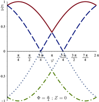
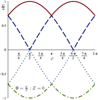
Figure 2: The spin-splitted ABS energy $E/\Delta$ in a S/N/S junction with a finite interface transparency versus the phase-difference $\varphi$, in the limit $\Phi\gg 2EL/v_{F}$ from Eq.(16). Left column: the strength of the interface $\delta$-barrier $Z=0$, right column: $Z=0.5$.

Previous results have been obtained assuming a perfect contact between the S electrodes and the N link. One can however generalize the Bohr-Sommerfeld quantization condition when adding scattering interfaces between the S and N materials Tinkham et al. (1982). Assuming the left (L) and right (R) interfaces with transmission probabilities $T_{L,R}=1-R_{L,R}$ and reflection coefficients $r_{L,R}$ with $\left|r_{L,R}\right|^{2}=R_{L,R}$ one obtains for a single channel junction (see SM):

$$\cos\left(\dfrac{2EL}{v_{F}}+s\Phi+2\theta\right)-\left(R_{R}+R_{L}\right)\cos\left(\dfrac{2EL}{v_{F}}+s\Phi\right)+\\ +R_{R}R_{L}\cos\left(\dfrac{2EL}{v_{F}}+s\Phi-2\theta\right)=\\ T_{L}T_{R}\cos\varphi-2\left(r_{L}r_{R}+r_{L}^{\ast}r_{R}^{\ast}\right)\sin^{2}\theta$$ (16)

for the condition of existence of ABS. Eq.(16) generalizes results known for the case of S/N/S systems without magnetic interactions; the case $\Phi=0$, $r_{L}=0$ has been obtained in Bagwell (1992). Supposing a strong enough magnetic texture, such that $\Phi\gg 2EL/v_{F}$, one can plot the ABS of a short Josephson junction for different junction transparency. As an example we consider a symmetric junction with $\delta$-barriers at the interfaces: $r_{L}=r_{R}=-\mathbf{i}Z/\left(1+\mathbf{i}Z\right)$, see Fig.2. In contrast to the case $\Phi=0$, where any finite barrier strength ($Z\neq 0)$ opens a gap, a finite $\Phi$ leads to a critical value of $Z$ below which zero-energy states exists. As one can infer by comparing the upper and lower rows of Fig. 2, this critical value of $Z$ increases by increasing $\Phi$.

In conclusion we have derived the semiclassical quantization condition for a S/N/S Josephson junction when the normal region exhibits generic SOC and exchange/Zeeman field. We obtained the spectrum of ABS Eq.(8), the quasiclassical Green’s function Eq.(10), and analyzed several physical observables in the presence of such generic spin-dependent field. We demonstrated that all the properties of the junction are expressed in terms of two fundamental parameters: $\Phi$ and $\boldsymbol{\mathfrak{n}}(x)$, see Fig.1. These two parameters have a clear semiclassical meaning. The unit vector $\boldsymbol{\mathfrak{n}}(x)$ describes the local spin quantization axis about which a classical spin precess at a constant latitude while propagating through the junction. The magnetic phase $\Phi$ corresponds to the mismatch of the precession angles after a quasiparticle completes the closed Andreev orbit. $\Phi$ enters explicitly the expression for the Josephson current, while $\boldsymbol{\mathfrak{n}}$ can be accessed experimentally by measuring the spin-resolved density of states. A magnetic Josephson junction can thus be used as an analog computer of path-ordered loop operators (3)-(6).

Appendix A Convention

The Green-Gor’kov functions read

$$\check{G}\left(x_{1},x_{2};t_{1},t_{2}\right)=\dfrac{1}{\mathbf{i}\hbar}\left\langle\hat{T}\left[\left(\begin{array}[]{c}\Psi\left(x_{1},t_{1}\right)\\ \left[\mathbf{i}\sigma_{2}\Psi\left(x_{1},t_{1}\right)\right]^{\dagger T}\end{array}\right)\right.\right.\\ \left.\left.\otimes\left(\begin{array}[]{cc}\Psi^{\dagger}\left(x_{2},t_{2}\right)&\left[\mathbf{i}\sigma_{2}\Psi\left(x_{2},t_{2}\right)\right]^{T}\end{array}\right)\right]\right\rangle$$ (17)

in the Nambu space, with

$$\Psi\left(x,t\right)=\left(\begin{array}[]{c}\Psi_{\uparrow}\\ \Psi_{\downarrow}\end{array}\right)$$ (18)

a spinor or annihilation operators of fermion with spin $\uparrow$ or $\downarrow$, respectively. $\Psi^{\dagger}$ is the creation spinor associated to $\Psi$ and ^T represent the transpose. $\hat{T}$ is the time-ordering operator, see Abrikosov et al. (1963).

The quasi-classic Green’s functions are defined as Langenberg and Larkin (1986)

$$\check{g}\left(x,t_{1},t_{2}\right)=\dfrac{\mathbf{i}}{\pi}\int d\xi\left[\check{G}\left(p,x,t_{1},t_{2}\right)\right]$$ (19)

where $\xi=v_{F}\left(p-p_{F}\right)$ is the linearised increment at the Fermi level, and $\check{G}\left(p,x\right)$ is obtained from $\check{G}\left(x_{1},x_{2}\right)$ by the usual semi-classic expansion, also known as Wigner transform or mixed coordinate Fourier transform Langenberg and Larkin (1986). Here we used a gauge-covariant generalisation of it, the details of which can be found in Bergeret and Tokatly (2014); Konschelle (2014), see also Gorini et al. (2010). One then defines

$$\check{g}=\left(\begin{array}[]{cc}g&f\\ \bar{f}&-\overline{g}\end{array}\right)$$ (20)

in the Nambu space, with

$$g=\left(\begin{array}[]{cc}g_{\uparrow\uparrow}&g_{\uparrow\downarrow}\\ g_{\downarrow\uparrow}&g_{\downarrow\downarrow}\end{array}\right)\;;\;f=\left(\begin{array}[]{cc}f_{\uparrow\downarrow}&f_{\uparrow\uparrow}\\ f_{\downarrow\downarrow}&f_{\downarrow\uparrow}\end{array}\right)$$ (21)

and so on for $\bar{f}=\mathcal{T}f\mathcal{T}^{-1}$ and $\bar{g}=\mathcal{T}g\mathcal{T}^{-1}$, with $\mathcal{T}$ the time reversal operation. The components $g_{\alpha\beta}$, $\alpha\in\left\{\uparrow,\downarrow\right\}$ are correlation functions, whereas $g$ and $f$ are matrices in the spin space (span by the $\sigma$’s Pauli matrices), and $\check{g}$ is a matrix in the Nambu space (span by the $\tau$’s Pauli matrices). In the main text we calculate the matrix $g$ in the spin space, see Eq.(9).

Appendix B Andreev-Wilson loop

Here we discuss basic properties of the Andreev-Wilson loop operators defined by Eqs. (2)-(3) of the main text. The goal of this part is to clarify the details of the semiclassical construction schematically drawn on Fig.1 in the article.

Our starting point is the semiclassical Bogoliubov-deGennes (BdG) equations (also known as Andreev approximation of the BdG equations)

$$-\mathbf{i}\boldsymbol{v\cdot\nabla}\psi+\boldsymbol{B}\left(\boldsymbol{v},x\right)\boldsymbol{\cdot\sigma}\psi+\Delta\chi =E\psi$$

$$\mathbf{i}\boldsymbol{v\cdot\nabla}\chi+\boldsymbol{B}\left(-\boldsymbol{v},x\right)\boldsymbol{\cdot\sigma}\chi+\Delta^{\ast}\psi =E\chi$$ (22)

for the spinor $\psi$ of the electron-like excitation and the spinor $\chi$ for a hole-like excitation, with $\Delta$ being the superconducting gap (assumed to be zero in the normal region), $\boldsymbol{B}$ a magnetic texture which depends on the Fermi velocity $\boldsymbol{v}$ and position $x$, and $E$ the excitation energy. Here, we assume that the system is translational invariant in the transversal direction and therefore $\boldsymbol{v\cdot\nabla}\equiv v\partial_{x}$, where the velocity $v=v_{F}\cos\phi,$ is parametrized by the angle between the semiclassical trajectory and the $x$-axis perpendicular to the S/N interfaces.

Note that the equations (22) correspond to the leading order of the semi-classic expansion of the BdG equations in the presence of any spin texture (spin splitting field plus spin-orbit coupling).

The operator $U\left(x_{2},x_{1}\right)$ defined in the main text is the spin propagator that connects the values of the electron-like spinor at two different points: $\psi\left(x_{2}\right)=e^{\mathbf{i}E\left(x_{2}-x_{1}\right)/v}U\left(x_{2},x_{1}\right)\psi\left(x_{1}\right)$. From the BdG equations we find that $U\left(x_{2},x_{1}\right)$ satisfies the following equations (in the N-region)

$$\mathbf{i}v\dfrac{\partial}{\partial x_{1}}U\left(x_{1},x_{2}\right) =\boldsymbol{B}\left(v,x_{1}\right)\boldsymbol{\cdot\sigma}U\left(x_{1},x_{2}\right)$$

$$\mathbf{i}v\dfrac{\partial}{\partial x_{2}}U\left(x_{1},x_{2}\right) =-U\left(x_{1},x_{2}\right)\boldsymbol{B}\left(v,x_{1}\right)\boldsymbol{\cdot\sigma}$$ (23)

with the boundary condition $U(x_{1},x_{1})=1$, and verifies the group property $U\left(x_{1},x_{3}\right)U\left(x_{3},x_{2}\right)=U\left(x_{1},x_{2}\right)$. The solution to these equations is given by the path-ordered exponential

$$U\left(x_{2},x_{1}\right)=\operatorname{Pexp}\left\{-\dfrac{\mathbf{i}}{v}\int_{x_{1}}^{x_{2}}\boldsymbol{B}\left(v,x\right)\boldsymbol{\cdot\sigma}dx\right\}$$ (24)

which is the Eq.(4) of the main text.

The spin propagator for the hole-like spinor is defined similarly as $\chi\left(x_{2}\right)=e^{-\mathbf{i}E\left(x_{2}-x_{1}\right)/v}\bar{U}\left(x_{2},x_{1}\right)\chi\left(x_{1}\right)$. It follows from the BdG equations (22) that operators $U$ and $\bar{U}$ are related via the time-reversal operation: $\bar{U}\left(v\right)=\sigma^{y}U^{\ast}\left(-v\right)\sigma^{y}$. Explicitly the path-ordered exponential representation for $\bar{U}\left(x_{2},x_{1}\right)$ reads

$$\bar{U}\left(x_{2},x_{1}\right)=\operatorname{Pexp}\left\{\dfrac{\mathbf{i}}{v}\int_{x_{1}}^{x_{2}}\boldsymbol{B}\left(-v,x\right)\boldsymbol{\cdot\sigma}dx\right\}.$$ (25)

Note that $U$ can be also obtained from $\bar{U}$ by simply reversing the velocity $\bar{U}(v)=U(-v)$, which reflects the electron-hole symmetry.

From the spin propagators $U$ and $\bar{U}$ we construct the Andreev-Wilson loop operators [Eqs.(2) and (3) of the main text]

$$W_{e}\left(x\right) =U\left(x,x_{L}\right)\bar{U}\left(x_{L},x_{R}\right)U\left(x_{R},x\right)$$ (26)

$$W_{h}(x) =\bar{U}\left(x,x_{R}\right)U\left(x_{R},x_{L}\right)\bar{U}\left(x_{L},x\right)\>.$$ (27)

These operators propagate electron-like and hole-like spinors in the particle-hole $\otimes$ position space along an Andreev loop between the two superconducting electrodes at locations $x_{L}$ and $x_{R}$ [see Fig.1, main text]. For example the operator $W_{e}(x)$ propagates the electron spinor from a point $x$ to the right interface at $x_{R}$, then the hole spinor from $x_{R}$ to the left interface at $x_{L}$, and finally it transfers the electron spinor from $x_{L}$ back to the original point $x$.

Since the above defined Andreev-Wilson loop operators are $\text{SU}\left(2\right)$ rotation matrices we can represent them in the following form

$$W_{e,h}\left(x\right) =\exp\left[\mathbf{i}\left(\boldsymbol{\mathfrak{n}}_{e,h}\left(x\right)\boldsymbol{\cdot\sigma}\right)\Phi\right]$$ (28)

$$=\cos\Phi+\mathbf{i}\left(\boldsymbol{\mathfrak{n}}_{e,h}\left(x\right)\boldsymbol{\cdot\sigma}\right)\sin\Phi\,,$$ (29)

where $\boldsymbol{\mathfrak{n}}_{e}\left(x\right)$ and $\boldsymbol{\mathfrak{n}}_{h}\left(x\right)$ are unit vectors. Using the group property of the propagators $U(x_{1},x_{2})$ and $\bar{U}(x_{1},x_{2})$ we find the relation

$$\operatorname{Tr}\left\{W_{e,h}\right\}=\operatorname{Tr}\left\{U\left(x_{R},x_{L}\right)\bar{U}\left(x_{L},x_{R}\right)\right\}=2\cos\Phi$$ (30)

which shows that the parameter $\Phi$ is $x$-independent and the same for the electron- and hole-like loop operators. In contrast to that the vectors $\boldsymbol{\mathfrak{n}}_{e}\left(x\right)$ and $\boldsymbol{\mathfrak{n}}_{h}\left(x\right)$ are in general different and $x$-dependent. The physical significance of the parametrization (28) is the following. When the expectation values of the electron $\mathbf{s}_{e}\left(x\right)=\psi^{\dagger}\left(x\right)\boldsymbol{\sigma}\psi\left(x\right)$ and hole $\mathbf{s}_{h}\left(x\right)=\chi^{\dagger}\left(x\right)\boldsymbol{\sigma}\chi\left(x\right)$ spin vectors are propagated around the Andreev-Wilson loops based at the point $x$, they rotate by the angle $\Phi$ about the directions of $\boldsymbol{\mathfrak{n}}_{e}\left(x\right)$ and $\boldsymbol{\mathfrak{n}}_{h}\left(x\right)$, respectively.

Using (23) and the definitions (26)-(27) we find the equations of motion for the Andreev-Wilson loop operators,

$$\mathbf{i}v\dfrac{\partial}{\partial x}W_{e}\left(x\right)=\mathbf{i}v\dfrac{\partial U\left(x,x_{L}\right)}{\partial x}\bar{U}\left(x_{L},x_{R}\right)U\left(x_{R},x\right)\\ +\mathbf{i}vU\left(x,x_{L}\right)\bar{U}\left(x_{L},x_{R}\right)\dfrac{\partial U\left(x_{R},x\right)}{\partial x}\\ =\left[\boldsymbol{B}\left(v,x\right)\boldsymbol{\cdot\sigma},W_{e}\left(x\right)\right]$$ (31)

and similarly for $W_{h}(x)$:

$$-\mathbf{i}v\partial_{x}W_{h}\left(x\right)=\left[\boldsymbol{B}\left(-v,x\right)\boldsymbol{\cdot\sigma},W_{h}\left(x\right)\right]\,.$$ (32)

By substituting the representation (29) into the relation (31) and recalling the property (30), one gets

$$\pm\mathbf{i}v\partial_{x}\left(\boldsymbol{\mathfrak{n}}_{e,h}\left(x\right)\boldsymbol{\cdot\sigma}\right)=\left[\boldsymbol{B}\left(\pm v,x\right)\boldsymbol{\cdot\sigma},\boldsymbol{\mathfrak{n}}_{e,h}\left(x\right)\boldsymbol{\cdot\sigma}\right]$$ (33)

Next, using the identity $\left(\boldsymbol{A\cdot\sigma}\right)\left(\boldsymbol{B\cdot\sigma}\right)=\boldsymbol{A\cdot B}+\mathbf{i}\left(\boldsymbol{A\times B}\right)\boldsymbol{\cdot\sigma}$ for $\boldsymbol{A}$ and $\boldsymbol{B}$ in $\mathbb{R}^{3}$ to evaluate the commutator, we eventually arrive at the following classical equations of precession of the vectors $\boldsymbol{\mathfrak{n}}_{e,h}$ around the effective magnetic field $\boldsymbol{B}$:

$$v\partial_{x}\boldsymbol{\mathfrak{n}}_{e} =2\boldsymbol{B}\left(v,x\right)\times\boldsymbol{\mathfrak{n}}_{e}$$

$$v\partial_{x}\boldsymbol{\mathfrak{n}}_{h} =-2\boldsymbol{B}\left(-v,x\right)\times\boldsymbol{\mathfrak{n}}_{h}$$ (34)

This corresponds to Eq.(6) of the main text.

To establish the boundary conditions for Eqs.(34) we evaluate the loop operators (26)-(27) at the interface points

$$W_{e}\left(x_{L}\right)=\bar{U}\left(x_{L},x_{R}\right)U\left(x_{R},x_{L}\right)=W_{h}\left(x_{L}\right)$$ (35)

$$W_{h}\left(x_{R}\right)=U\left(x_{R},x_{L}\right)\bar{U}\left(x_{L},x_{R}\right)=W_{e}\left(x_{R}\right)$$ (36)

These relations imply that $\boldsymbol{\mathfrak{n}}_{e}\left(x_{L,R}\right)=\boldsymbol{\mathfrak{n}}_{h}\left(x_{L,R}\right)$ at the interfaces with the superconducting electrodes, since $\Phi$ is position independent, see (30). Therefore, despite the Bogoliubov quasiparticles bouncing back at the S/N interfaces, $x=x_{L,R}$ and transmuting there (electron-like excitation becomes a hole-like excitation and vice-versa by the Andreev reflection), the local precession vectors $\boldsymbol{\mathfrak{n}}_{e}$ and $\boldsymbol{\mathfrak{n}}_{h}$ are equal at the interfaces, hence the propagation of the spinors $\psi$ and $\chi$ can be defined continuously along an Andreev loop.

Obviously the electron $\mathbf{s}_{e}\left(x\right)=\psi^{\dagger}\left(x\right)\boldsymbol{\sigma}\psi\left(x\right)$ and hole spin vector $\mathbf{s}_{h}\left(x\right)=\chi^{\dagger}\left(x\right)\boldsymbol{\sigma}\chi\left(x\right)$, also satisfy the precession equations similar to Eqs.(34). Hence one naturally expects that the scalar product $\mathbf{s}_{e,h}(x)\boldsymbol{\cdot\mathfrak{n}}_{e,h}(x)$ should be preserved along the loop. Indeed, using the BdG equations (22) and the relation (34) one has

$$\mathbf{i}v\dfrac{\partial\mathbf{s}_{e}\boldsymbol{\cdot\mathfrak{n}}_{e}}{\partial x}=\mathbf{i}v\dfrac{\partial\psi^{\dagger}}{\partial x}\boldsymbol{\sigma\cdot\mathfrak{n}}_{e}\psi+\mathbf{i}v\psi^{\dagger}\dfrac{\partial\boldsymbol{\sigma\cdot\mathfrak{n}}_{e}}{\partial x}\psi\\ +\mathbf{i}v\psi^{\dagger}\boldsymbol{\sigma\cdot\mathfrak{n}}_{e}\dfrac{\partial\psi}{\partial x}=-\psi^{\dagger}\left(\boldsymbol{B}\left(v\right)\boldsymbol{\cdot\sigma}\right)\left(\boldsymbol{\mathfrak{n}}_{e}\boldsymbol{\cdot\sigma}\right)\psi\\ +\psi^{\dagger}2\mathbf{i}\left(\boldsymbol{B}\left(v\right)\boldsymbol{\times\mathfrak{n}}_{e}\right)\boldsymbol{\cdot\sigma}\psi+\psi^{\dagger}\left(\boldsymbol{\mathfrak{n}}_{e}\boldsymbol{\cdot\sigma}\right)\left(\boldsymbol{B}\left(v\right)\boldsymbol{\cdot\sigma}\right)\psi\\ \Rightarrow\mathbf{i}v\dfrac{\partial\mathbf{s}_{e}\boldsymbol{\cdot\mathfrak{n}}_{e}}{\partial x}=0\;.$$ (37)

Here we have used that $\left(\boldsymbol{A\cdot\sigma}\right)\left(\boldsymbol{B\cdot\sigma}\right)=\boldsymbol{A\cdot B}+\mathbf{i}\left(\boldsymbol{A\times B}\right)\boldsymbol{\cdot\sigma}$ for $\boldsymbol{A}$ and $\boldsymbol{B}$ in $\mathbb{R}^{3}$. Similarly we find that $\mathbf{s}_{h}\boldsymbol{\cdot\mathfrak{n}}_{h}$ is also space independent. Thus the projection of the expectation value $\mathbf{s}_{e,h}(x)$ of the electron/hole spin on the local axis $\boldsymbol{\mathfrak{n}}_{e,h}(x)$ remains constant in the course of propagation along the closed Andreev trajectory. In other words, the spin dynamics can be viewed as a precession at a constant latitude about a local axis that itself changes along the trajectories according to Eq.(34). All this confirms the picture illustrated in Fig.1 in the main text.

Finally we note that, mathematically speaking, the constancy of the projection of the spin vector $\mathbf{s}_{e,h}(x)$ on the local axis $\boldsymbol{\mathfrak{n}}_{e,h}(x)$ means the existence of an extra integral of motion in the classical spin dynamics. This additional integral of motion allows to reduce the SU(2) holonomy (expected in the spin-1/2 problem) to an U(1) holomony parametrized by a single scalar parameter $\Phi$. A similar property has been identified by Keppeler in the context of semilassical quantization of spinning electrons described by Pauli or Dirac equations Keppeler (2003, 2002). Our results in fact show that the closed Andreev trajectory can be interpreted as a special case of the generalized invariant torus introduced in Refs.Keppeler (2003, 2002). The important difference is however that in our case $\Phi$ is the holonomy associated to the equations (23) along the path shown in Fig.1 (main text) mixing electron and hole trajectories. The non-integrable loop so formed exists in the particle-hole $\otimes$ position space.

Appendix C Josephson junction as an analog computer of path-ordered exponential

As discussed above, the Andreev-Wilson loop operators describe the spin dependency of the BdG bispinor (22) as they move along the normal region. The loop can not be defined only in the position space since this one is purely 1D along a quasi-classic trajectory, but in the particle-hole $\otimes$ position space. It is clear that without a time-reversal breaking field in the normal region, one has trivial operators $W_{e}=W_{h}=1$ and no $\Phi$-holonomy. There is in fact no loop in this case. So the surface of the loop is described by the amplitude of the time-reversal breaking field (which gives the difference between $U$ and $\bar{U}$) and the length of the junction. To recall this subtlety, we coined $W_{e,h}$ the Andreev-Wilson loop operators. They are not Wilson loop in the usual sense.

As described in the previous section of this supplemental materials, the Andreev-Wilson loop operators follow the usual equation of motion for the quantum state, providing we replace the usual time evolution – the Schrödinger equation – by the transport equation (23) for the evolution / displacement operator $U$.

An important problem for quantum information is to understand the time evolution of the qubit state. This evolution is defined as a time-ordered Dyson series, which usually require heavy computational power to be calculated, even in a perturbative way. We have shown in the main text that a Josephson junction with magnetic interaction is an analog computer for such complicated mathematical objects. In fact, the Andreev-Wilson operator can be completely described by the two parameters $\Phi$ and $\boldsymbol{\mathfrak{n}}_{e,h}$, and one can access these two parameters by measuring the current-phase relation and/or the density of state and the spin polarized density of states, see the main text. Extracting $\Phi$ and $\boldsymbol{\mathfrak{n}}_{e,h}$ from such measurements, one can measure the result of the Dyson equations (23) in an analog fashion.

The Josephson devices might be versatile enough, since either the spin-orbit or the spin-splitting interaction could be tuned via external gates voltages, mutual inductances, etc. In addition, the quantity $L/v$ plays in the spinor propagation of the S/N/S junction the role of the time in the usual Schrödinger equation ; $L/v$ can be tuned as well (though with more difficulties than the magnetic texture itself).

Note finally that the expression for the quasiclassical Green’s function (Eqs.(9-10) of the main text) is pretty generic: if instead of a spin field, one considers any other Lie group structure associated to the generator of the Lie algebra $\mathfrak{s}$, the generator will simply appear by the replacement $\boldsymbol{\sigma}\rightarrow\boldsymbol{\mathfrak{s}}$ in the expression for the Green function, as long as this algebra will commute with the Nambu structure. In particular, a generalization to the recently proposed SU(N) cold atomic gas is straightforward Banerjee et al. (2013).

Thus, in certain sense our study is just a first step toward a possible understanding of the complete analogy between the transport of electron spin in coherent structures and the time evolution of complex quantum systems.

Appendix D Junction with barriers

In this section, we demonstrate the general expression (16) of the main text for the spectrum of the Andreev bound states when the junction has some barriers. We first consider the scattering of particles and holes with $E<\Delta$ at a single interface between a normal metal (left half space) and a superconductor (right half space). Then we discuss the case of two interfaces in order to get the spectrum of the Andreev bound states. All this analysis is done for a single-channel junction.

Notice there are other approaches to avoid discussing pure ballistic transport in Josephson junction. Perhaps the simplest one we could think of would be to adopt a diffusive equation approach Bergeret and Tokatly (2014). This is let for future study. Other ways are to add a scattering region in the normal part of the junction Beenakker and van Houten (1991), or to add a barrier in the middle of the junction Bagwell (1992). Nevertheless, these approaches are not easy to handle in our case, since one would like to preserve the Andreev-Wilson loop. So we adopt the method of adding impurities only at the S/N and N/S interfaces.

D.1 Single interface problem

Let us thus model a finite transparency interface by a potential barrier in the normal region at the distance from the interface $l\ll\xi_{0}$ smaller than the coherence length. The reason is due to the impossibility to treat a microscopic barrier in the semi-classic approximation. One has to add a normal region at the distance $l\ll\xi_{0}$ where microscopic theory should be prefered, and recover the semi-classic limit at large scale $\xi_{0}$. The BdG bispinor reads

$$\left(\begin{array}[]{c}u\left(x\right)\\ v\left(x\right)\end{array}\right)=\left(\begin{array}[]{c}\psi_{+}\left(x\right)\\ \chi_{+}\left(x\right)\end{array}\right)e^{\mathbf{i}\mathbf{k\cdot r}}+\left(\begin{array}[]{c}\psi_{-}\left(x\right)\\ \chi_{-}\left(x\right)\end{array}\right)e^{-\mathbf{i}\mathbf{k\cdot r}}$$ (38)

where the slowly varying functions $\psi_{\pm}$ and $\chi_{\pm}$ are the electron and hole spinors for two Fermi points labeled by the indexes $+$ and $-$. Note that the states $\psi_{+}$ and $\chi_{-}$ correspond to the right moving quasiparticles (positive velocity), while $\psi_{-}$ and $\chi_{+}$ describe the left movers (negative velocity). The barrier in the N-region is parametrized by the transmission $t$ and the reflection $r$ coefficients, which satisfy the following identities

$$\left|t\right|^{2}+\left|r\right|^{2} = 1$$ (39)

$$tr^{*}+t^{*}r = 0$$ (40)

It is convenient to introduce the electron and hole bispinors

$$\Psi=\left(\begin{array}[]{c}\psi_{+}\\ \psi_{-}\end{array}\right)\;\text{and}\;\Phi=\left(\begin{array}[]{c}\chi_{+}\\ \chi_{-}\end{array}\right)$$ (41)

and the transmission and reflection matrices

$$\hat{\mathbf{t}}=\left(\begin{array}[]{cc}t&0\\ 0&t^{*}\end{array}\right)\;\text{and}\;\hat{\textbf{r}}=\left(\begin{array}[]{cc}0&r\\ r^{*}&0\end{array}\right)$$ (42)

which satisfy the relations

$$\hat{\mathbf{t}}\hat{\mathbf{t}}^{\ast}=\left|t\right|^{2},\quad\hat{\textbf{r}}^{2}=\left|r\right|^{2},\quad\hat{\textbf{r}}\hat{\mathbf{t}}=-\hat{\mathbf{t}}\hat{\textbf{r}}^{\ast}$$ (43)

Importantly, the barrier scattering is the same for the electrons and holes as this is a Fermi surface property related to the fast oscillating parts of the BdG bispinors.

Then the scattering relation between the states on the right (labeled ^R) and on the left (labeled ^L) sides of the barrier can be written as follows.

$$\Psi^{R} = \hat{\textbf{r}}\Psi^{R}+\hat{\mathbf{t}}\Psi^{L}$$ (44)

$$\Phi^{R} = \hat{\textbf{r}}\Phi^{R}+\hat{\mathbf{t}}\Phi^{L}$$ (45)

From these relations we can construct the left-to-right transfer matrix defined as $\Psi^{R}=T\Psi^{L}$

$$\Psi^{R} =\left(1-\hat{\textbf{r}}\right)^{-1}\hat{\mathbf{t}}\Psi^{L}$$

$$=\left(1+\hat{\textbf{r}}\right)\frac{\hat{\mathbf{t}}}{\left|t\right|^{2}}\Psi^{L}=\frac{\hat{\mathbf{t}}}{\left|t\right|^{2}}\left(1-\hat{\textbf{r}}^{\ast}\right)\Psi^{L}$$ (46)

using the matrix identities (43). Therefore the transfer matrix is identified as

$$T=(1+\hat{\textbf{r}})\frac{\hat{\mathbf{t}}}{\left|t\right|^{2}}=\frac{\hat{\mathbf{t}}}{\left|t\right|^{2}}(1-\hat{\textbf{r}}^{\ast})$$ (47)

Using Eqs.(43) and (47) one can check that $TT^{*}=1$. Therefore the right-to-left transfer is described by $T^{*},$ that is $\Psi^{L}=T^{*}\Psi^{R}$.

The transfer matrices for the hole states are given by the same formulas.

The scattering of the states located between the barrier and the S-region (the states $\Psi^{R}$ and $\Phi^{R}$ in our case) is the pure Andreev scattering at the ideal fully transparent N/S interface

$$\Phi^{R}=S_{0}\Psi^{R},\;S_{0}=e^{-\mathbf{i}\varphi}\left(\begin{array}[]{cc}e^{-\mathbf{i}\theta}&0\\ 0&e^{\mathbf{i}\theta}\end{array}\right)$$ (48)

where $\varphi$ is the SC phase and $\theta=\arccos\frac{E}{\Delta}$, see e.g. Beenakker and van Houten (1991).

In the presence of the barrier the generalized Andreev scattering from the electrons to the holes on the left-hand-side of the barrier, $\Psi^{L}\to\Phi^{L}$, is composed from the two transfers across the barrier (forward L-to-R for electrons, and back R-to-L for holes) and a pure Andreev scattering in between: $\Psi^{L}\to\Psi^{R}\to\Phi^{R}\to\Phi^{L}$. This process is described as follows

$$\Phi^{L}=T^{*}S_{0}T\Psi^{L}\equiv A\Psi^{L}$$ (49)

Explicitly for the generalized Andreev scattering matrix we get

$$A = (1+\hat{\mathbf{r}}^{\ast})\frac{\hat{\mathbf{t}}^{\ast}}{\left|t\right|^{2}}S_{0}\frac{\hat{\mathbf{t}}}{\left|t\right|^{2}}(1-\hat{\mathbf{r}}^{\ast})=(1+\hat{\mathbf{r}}^{\ast})\frac{S_{0}}{\left|t\right|^{2}}(1-\hat{\mathbf{r}}^{\ast})$$ (52)

$$= \frac{e^{-\mathbf{i}\varphi}}{\left|t\right|^{2}}\left(\begin{array}[]{cc}e^{-\mathbf{i}\theta}-\left|r\right|^{2}e^{\mathbf{i}\theta}&r^{*}\left(e^{\mathbf{i}\theta}-e^{-\mathbf{i}\theta}\right)\\ r\left(e^{-\mathbf{i}\theta}-e^{\mathbf{i}\theta}\right)&e^{\mathbf{i}\theta}-\left|r\right|^{2}e^{-\mathbf{i}\theta}\end{array}\right)$$

The matrix $A$ connects the electron and hole states scattered by a non ideal N/S interface modeled by the barrier and an ideal N/S interface. In the following we will skip the index ^L, since the solutions are now all in the left/normal region, thus we have:

$$\left(\begin{array}[]{c}\chi_{+}\\ \chi_{-}\end{array}\right)=\\ \frac{e^{-\mathbf{i}\varphi}}{\left|t\right|^{2}}\left(\begin{array}[]{cc}e^{-\mathbf{i}\theta}-\left|r\right|^{2}e^{\mathbf{i}\theta}&r^{*}\left(e^{\mathbf{i}\theta}-e^{-\mathbf{i}\theta}\right)\\ r\left(e^{-\mathbf{i}\theta}-e^{\mathbf{i}\theta}\right)&e^{\mathbf{i}\theta}-\left|r\right|^{2}e^{-\mathbf{i}\theta}\end{array}\right)\left(\begin{array}[]{c}\psi_{+}\\ \psi_{-}\end{array}\right)$$ (53)

As the final step one can construct the interface scattering matrix $S$ which connects the right moving incident (electron and hole in the N region) states to the left moving reflected (electron and hole in the N region) states:

$$\left(\begin{array}[]{c}\psi_{-}\\ \chi_{+}\end{array}\right)=S\left(\begin{array}[]{c}\psi_{+}\\ \chi_{-}\end{array}\right)$$ (54)

The elements of the interface $S$ matrix are constructed from Eqs.(53) by expressing $\psi_{-}$ and $\chi_{+}$ in terms of $\psi_{+}$ and $\chi_{-}$. The resulting scattering matrix takes the form

$$S=\frac{1}{e^{\mathbf{i}\theta}-\left|r\right|^{2}e^{-\mathbf{i}\theta}}\left(\begin{array}[]{cc}r\left(e^{\mathbf{i}\theta}-e^{-\mathbf{i}\theta}\right)&\left|t\right|^{2}e^{\mathbf{i}\varphi}\\ \left|t\right|^{2}e^{-\mathbf{i}\varphi}&r^{*}\left(e^{\mathbf{i}\theta}-e^{-\mathbf{i}\theta}\right)\end{array}\right)\\ \equiv\left(\begin{array}[]{cc}r_{e}&r_{A}e^{\mathbf{i}\varphi}\\ r_{A}e^{-\mathbf{i}\varphi}&r_{h}\end{array}\right)$$ (55)

where we introduced the notations $r_{e}$ , $r_{h}$ for the electron and hole normal reflection coefficients and $r_{A}$ for the Andreev (electron-hole) reflection coefficient

$$r_{A} = \frac{\left|t\right|^{2}}{e^{\mathbf{i}\theta}-\left|r\right|^{2}e^{-\mathbf{i}\theta}}$$ (56)

$$r_{e} = r\frac{e^{\mathbf{i}\theta}-e^{-\mathbf{i}\theta}}{e^{\mathbf{i}\theta}-\left|r\right|^{2}e^{-\mathbf{i}\theta}}$$ (57)

$$r_{h} = r^{*}\frac{e^{\mathbf{i}\theta}-e^{-\mathbf{i}\theta}}{e^{\mathbf{i}\theta}-\left|r\right|^{2}e^{-\mathbf{i}\theta}}$$ (58)

One can verify that $\left|r_{A}\right|^{2}+\left|r_{e,h}\right|^{2}=1$, and the interface $S$-matrix is unitary $S^{\dagger}S=1.$

It seems to be quite obvious that in the case of an S/N interface (S on the left, N on the right), the same S-matrix (55) connects the left moving (incoming) states $\psi_{-}$ and $\chi_{+}$ to the right moving (reflected) states $\psi_{+}$ and $\chi_{-}$ (the incoming and outgoing are interchanged for S/N with respect to N/S).

D.2 Andreev bound states spectrum

In the Andreev bound states problem we have two interfaces (L and R) with $S$-matrices $S_{R}$ and $S_{L}$ given by Eq.(55) where the barrier transmission/reflection and the SC phases are in general different for L and R interfaces. The propagation between interfaces is diagonal in the electron-hole space (the same for either left movers and time-conjugated for right movers) and can be diagonalized locally in the spin space. As a result the single-valuedness condition (for the loop starting at the left boundary) reduces to the following simple form:

$$S_{L}S_{R}e^{\mathbf{i}\left(\frac{2E}{v}L+s\Phi\right)}\left(\begin{array}[]{c}\psi_{+}(x_{L})\\ \chi_{-}(x_{L})\end{array}\right)=\left(\begin{array}[]{c}\psi_{+}(x_{L})\\ \chi_{-}(x_{L})\end{array}\right)$$ (59)

Thus the problem reduces to a simple $2\times 2$ system (for each spin projection $s=\pm 1$) with a very clear physical meaning – the phase accumulated in the free closed loop propagation should be compensated by the combined scattering on two interfaces. The matrix in the r.h.s. is the generalization of our Andreev-Wilson loop to the case of general interfaces with finite transparency.

To obtain the spectrum of the Andreev bound states, one should thus resolve the condition

$$\det\left(1-S_{L}S_{R}e^{\mathbf{i}\left(\frac{2E}{v}L+s\Phi\right)}\right)=0$$ (60)

in order to get non-trivial solution verifying (59). After a straightforward calculation of the determinant and some algebra one obtains Eq.(16) of the main text.

Eq.(16) is quite generic since it is valid for any interface with all properties encoded in the expressions for $r$ and $t$ and any spin texture, encoded in the $\Phi$-holonomy. Eq.(16) thus generalizes many results scattered in the existing literature about single-channel Josephson junction, either for the S/N/S or the S/F/S problems.

References

- Buzdin (2005) A. I. Buzdin, Reviews of Modern Physics 77, 935 (2005).
- Bergeret et al. (2005) F. S. Bergeret, A. F. Volkov, and K. B. Efetov, Reviews of Modern Physics 77, 1321 (2005).
- Eschrig (2011) M. Eschrig, Physics Today 64, 43 (2011).
- Linder and Robinson (2015) J. Linder and J. W. A. Robinson, Nature Physics 11, 307 (2015), arXiv:1510.00713 .
- Franz (2013) M. Franz, Nature nanotechnology 8, 149 (2013).
- Beenakker (1997) C. Beenakker, Reviews of Modern Physics 69, 731 (1997), arXiv:9612179 [cond-mat] .
- Furusaki and Tsukada (1991) A. Furusaki and M. Tsukada, Solid State Communications 78, 299 (1991).
- Della Rocca et al. (2007) M. L. Della Rocca, M. Chauvin, B. Huard, H. Pothier, D. Esteve, and C. Urbina, Physical Review Letters 99, 127005 (2007).
- Bretheau et al. (2013) L. Bretheau, Ç. Ö. Girit, H. Pothier, D. Esteve, and C. Urbina, Nature 499, 312 (2013).
- Janvier et al. (2015) C. Janvier, L. Tosi, L. Bretheau, C. O. Girit, M. Stern, P. Bertet, P. Joyez, D. Vion, D. Esteve, M. F. Goffman, H. Pothier, and C. Urbina, Science 349, 1199 (2015), arXiv:1509.03961 .
- Abrikosov (1988) A. A. Abrikosov, Fundamentals of the theory of metals (North-Holland, 1988).
- Messiah (1995) A. Messiah, M’{e}canique quantique (Dunod (French reprint of the 1958 edition), 1995).
- Andreev (1964) A. F. Andreev, Sov. Phys. JETP 19, 1228 (1964).
- Note (1) In the strict semiclassical limit, i.e. , is the usual Maslov index at a turning point Duncan and Györffy (2002).
- Beenakker and van Houten (1991) C. Beenakker and H. van Houten, Physical Review Letters 66, 3056 (1991).
- Keppeler (2002) S. Keppeler, Physical Review Letters 89, 210405 (2002), arXiv:0207095 [quant-ph] .
- Keppeler (2003) S. Keppeler, Annals of Physics 304, 40 (2003), arXiv:0212082 [quant-ph] .
- Keppeler and Winkler (2002) S. Keppeler and R. Winkler, Phys. Rev. Lett. 88, 046401 (2002).
- Note (2) We assume the validity of the semiclassical approach. This means that we assume that all lengths and involved in the problem are larger than the Fermi wave length and all energies, in particular the SOC and Zeeman splitting, are smaller than the Fermi energy.
- Note (3) Time-reversal conjugation of an operator is given by .
- Note (4) In the non-Abelian gauge theory a path-ordered exponential describing a parallel transport of a spinor field over a closed loop in the real space is called a Wilson operator, and its trace is called a Wilson loop Peskin and Schroeder (1995). (3\@@italiccorr) and (4\@@italiccorr) also represent the transport along a loop, now generated by the Andreev reflections, and thus closes only in the combined position particle-hole space. To recall this subtlety, we call the Andreev-Wilson (AW) loop operators.
- Note (5) See Supplemental Material at [URL will be inserted by publisher] for a statement of the mathematical conventions followed in this study, the mathematical structure behind Fig.1, a lengthy discussion of the detection of the Andreev-Wilson loop and the derivation of Eq.(16\@@italiccorr).
- Note (6) The fact that only a non-zero Zeeman field leads to the spin splitting of the ABS is a consequence of the leading order semiclassical approximation. Beyond this approximation a lifting of the spin degenerancy can be achieved only by SOC , see e.g. Dimitrova and Feigel’man (2006) if the phase difference is non-zero. This is directly linked to the appearance of a finite magnetic moment by passing a current through weak link with SOC Konschelle et al. (2015).
- Bulaevskii et al. (1982) L. Bulaevskii, A. I. Buzdin, and S. Panjukov, Solid State Communications 44, 539 (1982).
- Buzdin et al. (1982) A. I. Buzdin, L. Bulaevskii, and S. V. Panyukov, Sov. Phys. JETP 35, 178 (1982).
- Blanter and Hekking (2004) Y. M. Blanter and F. W. J. Hekking, Physical Review B 69, 024525 (2004), arXiv:0306706 [cond-mat] .
- Bergeret and Tokatly (2014) F. S. Bergeret and I. V. Tokatly, Physical Review B 89, 134517 (2014), arXiv:1402.1025 .
- Konschelle (2014) F. Konschelle, The European Physical Journal B 87, 119 (2014), arXiv:1403.1797 .
- Konschelle et al. (2015) F. Konschelle, I. V. Tokatly, and F. S. Bergeret, Physical Review B 92, 125443 (2015), arXiv:1506.02977 .
- Reeg and Maslov (2015) C. R. Reeg and D. L. Maslov, , 26 (2015), arXiv:1508.03623 .
- Note (7) Details of the derivation will be given elsewhere, see also Konschelle et al. (2015) for similar calculations.
- Golubov et al. (2004) A. Golubov, M. Kupriyanov, and E. Il’ichev, Reviews of Modern Physics 76, 411 (2004).
- Konschelle et al. (2008) F. Konschelle, J. Cayssol, and A. I. Buzdin, Physical Review B 78, 134505 (2008), arXiv:0807.2560 .
- Pillet et al. (2010) J.-D. Pillet, C. H. L. Quay, P. Morfin, C. Bena, A. L. Yeyati, and P. Joyez, Nature Physics 6, 965 (2010).
- Tinkham et al. (1982) M. Tinkham, G. Blonder, and T. M. Klapwijk, Physical Review B 25, 4515 (1982).
- Bagwell (1992) P. Bagwell, Physical Review B 46, 12573 (1992).
- Abrikosov et al. (1963) A. A. Abrikosov, L. P. Gor’kov, and I. E. Dzyaloshinsky, Methods of quantum field theory in statistical physics (Prentice Hall, 1963).
- Langenberg and Larkin (1986) D. N. Langenberg and A. I. Larkin, Nonequilibrium superconductivity (North-Holland, Amsterdam, 1986).
- Gorini et al. (2010) C. Gorini, P. Schwab, R. Raimondi, and A. L. Shelankov, Physical Review B 82, 195316 (2010), arXiv:1003.5763 .
- Banerjee et al. (2013) D. Banerjee, M. Bögli, M. Dalmonte, E. Rico, P. Stebler, U.-J. Wiese, and P. Zoller, Physical Review Letters 110, 125303 (2013).
- Duncan and Györffy (2002) K. Duncan and B. Györffy, Annals of Physics 298, 273 (2002).
- Peskin and Schroeder (1995) M. E. Peskin and D. V. Schroeder, An introduction to quantum field theory (Westview Press, 1995).
- Dimitrova and Feigel’man (2006) O. V. Dimitrova and M. V. Feigel’man, Journal of Experimental and Theoretical Physics 102, 652 (2006).