Augmenting WFIRST Microlensing With A Ground-Based Telescope Network

1 Introduction

The proposed WFIRST mission (Spergel et al., 2015) contains a significant microlensing component, which will plausibly consist of six roughly 72-day continuous campaigns with 15 minute cadence covering about $2.8\,\rm deg^{2}$ of the Galactic Bulge. The observations will be made from L2 orbit and each campaign will be centered on quadrature, i.e., roughly March 21 and September 21. The observations will be carried out in a broad $H$-band, which is substantially less affected by dust than optical bands. In principle, this permits observations closer to the Galactic plane where the microlensing event rate is almost certainly higher than in the lowest-latitude fields accessible to ground-based $I$-band microlensing surveys.

The full power of a space-based survey at L2 can only be realized by complementing it with a deep, high-cadence, near continuous survey, as previous studies have suggested. Gould et al. (2003), Han et al. (2004), and Yee (2013) have previously discussed the possibility of microlens parallax measurements by combining observations from Earth and L2 orbit. Han et al. (2004) demonstrated that combining large format surveys from these two locations would yield microlens parallaxes and so mass measurements for low-mass objects, particularly FFPs. Yee (2013) focused on the specific challenges of conducting such parallax observations using WFIRST.

In this work, we provide a quantitative analysis of how the success of WFIRST microlensing experiment can be enhanced by complementary ground-based survey observations. The value of the so-called one-dimensional (1-D) parallax measurements is discussed. These will be substantially more plentiful than the 2-D parallaxes and, more importantly, measurable at all Einstein timescales. We also point out two additional benefits that such ground-based survey observations can provide to WFIRST.

In our calculations, we assume these ground-based observations are taken by a survey similar to the Korean Microlensing Telescope Network (KMTNet, Kim et al., 2016; Henderson et al., 2014). We recognize that adopting such an optical survey comes with a loss in event rate, as it requires that WFIRST be pointed at lower-extinction fields than is currently envisaged. Therefore, the benefits of adopting such a survey must be weighed against such a cost. Our methodology can be easily adapted for any specified microlensing surveys, either ongoing or planned.

2 Microlensing Parallaxes

The standard microlensing light curve normally only yields one single observable that is of physical interest, the event timescale $t_{\rm E}$,

$$t_{\rm E}\equiv\frac{\theta_{\rm E}}{\mu_{\rm rel}}\ .$$ (1)

Here $\mu_{\rm rel}=|\mbox{\boldmath$\mu$}_{\rm rel}|$ is the relative proper motion between the lens and the source, and $\theta_{\rm E}$ is the angular Einstein radius

$$\theta_{\rm E}\equiv\sqrt{\kappa M_{\rm L}\pi_{\rm rel}}\ ,$$ (2)

where $\kappa\equiv 4G/(c^{2}{\rm AU})$ and $\pi_{\rm rel}={\rm AU}(D_{\rm L}^{-1}-D_{\rm S}^{-1})$ is the lens-source relative parallax. Here $D_{\rm L}$ and $D_{\rm S}$ are the distances to the lens and the source, respectively.

Under certain circumstances, the microlens parallax effect can be measured, which yields the microlens parallax parameter,

$${\mbox{\boldmath$\pi$}}_{\rm E}\equiv\pi_{\rm E}\frac{{\mbox{\boldmath$\mu$}}_{\rm rel}}{\mu_{\rm rel}};\quad\pi_{\rm E}\equiv\frac{\pi_{\rm rel}}{\theta_{\rm E}}\ .$$ (3)

This can be done by using a single accelerating observatory (Gould, 1992), or by taking observations simultaneously from two separated sites (Refsdal, 1966; Gould, 1994b; Holz & Wald, 1996; Gould, 1997). In the latter case, the microlens parallax vector is given by

$${\mbox{\boldmath$\pi$}}_{\rm E}=\frac{{\rm AU}}{D_{{\rm sat},\perp}}\left(\frac{\Delta t_{0}}{t_{\rm E}},\Delta u_{0}\right)\ ,$$ (4)

where $D_{{\rm sat},\perp}$ is the projected separation between the two observatories evaluated at the peak of the event, and $\Delta t_{0}=t_{0,{\rm sat}}-t_{0,\oplus}$ and $\Delta u_{0}=u_{0,{\rm sat}}-u_{0,\oplus}$ are the differences in the peak times and impact parameters as seen from the two observatories (we have assumed Earth and one satellite), respectively.

In many cases, however, only the component of the vector ${\mbox{\boldmath$\pi$}}_{\rm E}$ parallel to the opposite direction of acceleration (i.e., away from the Sun for Earth and WFIRST) projected onto the sky can be measured with reasonable precision. This component is denoted as $\pi_{{\rm E},\parallel}$

$$\pi_{{\rm E},\parallel}\equiv{\mbox{\boldmath$\pi$}}_{\rm E}\cdot\hat{\bf n}\equiv\pi_{\rm E}\cos\phi_{\pi}\ ,$$ (5)

where $\hat{\bf n}$ is the opposite direction of acceleration projected on the sky, and $\phi_{\pi}$ is the angle between ${\mbox{\boldmath$\pi$}}_{\rm E}$ and $\hat{\bf n}$.

The parameters $\pi_{{\rm E},\parallel}$ and ${\mbox{\boldmath$\pi$}}_{\rm E}$ are often called 1-D and 2-D parallaxes, respectively.

To facilitate later discussions, we introduce the vector microlensing parameter $\Lambda$ (Dong et al., 2007)

$$\mbox{\boldmath$\Lambda$}\equiv\frac{t_{\rm E}{\mbox{\boldmath$\pi$}}_{\rm E}}{{\rm AU}}={\pi_{\rm rel}/\mu_{\rm rel}\over{\rm AU}}\,{{\mbox{\boldmath$\mu$}}_{\rm rel}\over\mu_{\rm rel}},$$ (6)

whose amplitude $\Lambda=1/\tilde{v}$ is the reciprocal of the projected transverse velocity. Because $\Lambda$ is a purely kinematic quantity, it can be used to distinguish between disk events (disk lens + Bulge source) and Bulge events (Bulge lens + Bulge source) (Gould et al., 1994). That is, its (inverse) amplitude is typically

$$\tilde{v}=\left\{\begin{array}[]{ll}280{\rm km~{}s^{-1}}&{,\ \rm Disk~{}events}\cr 1000{\rm km~{}s^{-1}}&{,\ \rm Bulge~{}events}\end{array}\right.$$ (7)

Here we have adopted $\pi_{\rm rel}=0.12~{}{\rm mas}$ and $\mu_{\rm rel}=7~{}{\rm mas}\,{\rm yr}^{-1}$ as typical values for disk events, and $\pi_{\rm rel}=0.02~{}{\rm mas}$ and $\mu_{\rm rel}=4~{}{\rm mas}\,{\rm yr}^{-1}$ for Bulge events.

In the satellite parallax method, $\Lambda$ is more directly measured than ${\mbox{\boldmath$\pi$}}_{\rm E}$ (Equation (4))

$$\mbox{\boldmath$\Lambda$}=\frac{1}{D_{{\rm sat},\perp}}\left(\Delta t_{0},t_{\rm E}\Delta u_{0}\right)\ ,$$ (8)

because $\Delta t_{0}$ is usually better measured than $t_{\rm E}$. Moreover, as we will show below, for the special case of L2 space parallaxes (as well as terrestrial parallaxes, Gould & Yee 2013) $t_{\rm E}\Delta u_{0}\rightarrow\Delta t_{\rm eff}$ where $t_{\rm eff}\equiv u_{0}t_{\rm E}$, and $t_{\rm eff}$ can be much better measured than $t_{\rm E}$. This is especially true for short timescale events, as $t_{\rm E}$ and $u_{0}$ can be severely degenerate with each other as well as other parameters such as the source flux $F_{\rm s}$.

3 WFIRST+Ground Parallaxes

Whenever there are microlens parallax measurements from comparing the light curves of two observatories, it is also possible to obtain complementary parallax information from the accelerated motion of one or both observatories separately. In the present case, WFIRST orbital parallax will play a major complementary role to the two-observatory parallaxes that are made possible by a ground-based observatory (or network of ground-based observatories). However, for clarity, we begin by analyzing the parallax information that can be derived by comparing the two light curves.

WFIRST-Earth microlensing has some features that differ substantially from those two-observatory experiments that have been carried out previously or that are being carried out. First, since WFIRST is a dedicated space-based photometry experiment, it will almost always have essentially perfect measurements relative to the ground. Therefore, the errors in the parallax measurements are very well approximated as those due to the ground observations. Second, for similar reasons, WFIRST-selected events will be quite faint as seen from Earth, and therefore the Earth-based photometry errors can be treated as “below sky”, i.e., independent of flux. Third, since WFIRST will be at L2, its projected motion relative to Earth will be extremely slow, substantially less than $1\,{\rm km~{}s^{-1}}$. This can be compared with typical lens-source projected velocities $\tilde{v}\sim{\cal O}(100\,{\rm km~{}s^{-1}})$. This means that the Einstein timescales $t_{\rm E}$ are essentially identical as seen from the two locations. In particular, it implies that the quantity entering $\Lambda_{\perp}=t_{\rm E}\Delta u_{0}/D_{\rm sat,\perp}$ can be simplified by

$$t_{\rm E}\Delta u_{0}=\Delta(u_{0}t_{\rm E})-u_{0}\Delta t_{\rm E}\rightarrow\Delta t_{\rm eff}$$ (9)

where $t_{\rm eff}\equiv u_{0}t_{\rm E}$. That is, Equation (8) becomes

$$\mbox{\boldmath$\Lambda$}\rightarrow\frac{1}{D_{{\rm sat},\perp}}\left(\Delta t_{0},\Delta t_{\rm eff}\right)\ ,$$ (10)

as we anticipated above. In addition, in most cases, $t_{\rm E}$ will in fact be measured from WFIRST even if it cannot be measured from Earth, so that we can then convert ${\mbox{\boldmath$\pi$}}_{\rm E}=({\rm AU}/t_{\rm E}){\mbox{\boldmath$\Lambda$}}$. From our standpoint, we will therefore regard measurement of $\Lambda$ as the goal, with the understanding that this itself will very often yield ${\mbox{\boldmath$\pi$}}_{\rm E}$. And even when it cannot, $\Lambda$ is the crucial parameter for distinguishing populations in any case because it is a purely kinematic variable. Finally, since WFIRST will be at L2, WFIRST-Earth parallaxes are exceptionally sensitive to short events, which is traditionally the most difficult regime, i.e., the regime of events generated by very low-mass lenses. That is, such events do not last long enough to make orbital parallax measurements, and their Einstein radii are too small to permit simultaneous observation from observatories separated by $\sim{\rm AU}$, like Spitzer and Kepler.

We analyze the WFIRST-ground parallaxes using Fisher matrices. The full point-lens equation is described by four parameters that are of physical interest, $a_{i}=(t_{0},u_{0},t_{\rm E},F_{\rm s})$, and one nuisance parameter $F_{\rm base}$

$$F(t)=F_{\rm s}(A[u(t)]-1)+F_{\rm base}\ ,$$ (11)

where

$$A(u)=\frac{u^{2}+2}{u\sqrt{u^{2}+4}}\ ;\quad u^{2}=\tau^{2}+u_{0}^{2}\ ;\quad\tau\equiv\frac{t-t_{0}}{t_{\rm E}}\ .$$ (12)

The nuisance parameter $F_{\rm base}$ is essentially uncorrelated with other parameters, so we ignore it in the following analysis. Under the assumption of uniform observations at a cadence $\Gamma$, the Fisher matrix (i.e., inverse of the covariance matrix) is then given by

$$b_{ij}=\frac{\Gamma}{\sigma_{0}^{2}}\int_{-\infty}^{+\infty}dt\frac{\partial F(t)}{\partial a_{i}}\frac{\partial F(t)}{\partial a_{j}}\ ,$$ (13)

where we have assumed that the observations are below sky so that the flux error $\sigma_{0}$ is independent of magnification. Here

$$\frac{\partial F}{\partial a_{i}}=\left(\begin{array}[]{c}-F_{\rm s}A^{\prime}\tau/(ut_{\rm E})\cr F_{\rm s}A^{\prime}u_{0}/u\cr-F_{\rm s}A^{\prime}\tau^{2}/(ut_{\rm E})\cr A-1\cr\end{array}\right)\ ,$$ (14)

and

$$A^{\prime}\equiv\frac{dA}{du}=\frac{-8}{u^{2}(u^{2}+4)^{3/2}}\ .$$ (15)

Although the Fisher matrix cannot be expressed in closed form for the general case, it can be in the high magnification regime, where $A(u)=1/u$ and $A^{\prime}(u)=-1/u^{2}$. Below we derive these closed-form expressions in this regime, and provide the analysis of the general case in Appendix A.

In the high-magnification limit, it can be seen that

$$u_{0}\frac{\partial F}{\partial u_{0}}-t_{\rm E}\frac{\partial F}{\partial t_{\rm E}}+F_{\rm s}\left(\frac{\partial F}{\partial F_{\rm s}}+1\right)=0\ .$$ (16)

That is, in this limiting regime, the parameters $(u_{0},t_{\rm E},F_{\rm s})$ are degenerate. Hence, the only way to distinguish them is from the wings of the light curve. This can be a serious problem for ground-based observations of WFIRST targets, since they may be extremely faint and noisy near baseline.

However, as stated above we are not actually interested in directly measuring $t_{\rm E}$ from the ground. We therefore rewrite Equations (11) and (12) in the high-magnification limit, which has only three parameters (Gould, 1996) $a_{i}=(t_{0},t_{\rm eff},F_{\rm peak})$

$$F(t)=F_{\rm peak}Q(t)\ ;\qquad Q(t)=\biggl{(}{(t-t_{0})^{2}\over t_{\rm eff}^{2}}+1\biggr{)}^{-1/2}\ .$$ (17)

Then

$${\partial F\over\partial a_{i}}\rightarrow\left(\matrix{F_{\rm peak}Q^{3}\tau_{\rm eff}/t_{\rm eff}\cr F_{\rm peak}Q^{3}\tau_{\rm eff}^{2}/t_{\rm eff}\cr Q}\right)\ ,$$ (18)

where $\tau_{\rm eff}\equiv(t-t_{0})/t_{\rm eff}$. We then evaluate the inverse covariance matrix,

$$b_{ij}={\pi\over 8}{\Gamma t_{\rm eff}F_{\rm peak}^{2}\over\sigma_{0}^{2}}\left(\matrix{t_{\rm eff}^{-2}&0&0\cr 0&3t_{\rm eff}^{-2}&4t_{\rm eff}^{-1}F_{\rm peak}^{-1}\cr 0&4t_{\rm eff}^{-1}F_{\rm peak}^{-1}&8F_{\rm peak}^{-2}}\right)\ ,$$ (19)

and thus the covariance matrix $c=b^{-1}$

$$c_{ij}={8\over\pi}{\sigma_{0}^{2}\over F_{\rm peak}^{2}\Gamma t_{\rm eff}}\left(\matrix{t_{\rm eff}^{2}&0&0\cr 0&t_{\rm eff}^{2}&-t_{\rm eff}F_{\rm peak}/2\cr 0&-t_{\rm eff}F_{\rm peak}/2&(3/8)F_{\rm peak}^{2}}\right)\ .$$ (20)

Thus the uncertainties on $t_{0}$ and $t_{\rm eff}$ are

$$\sigma(t_{0})=\sqrt{{8\over\pi}\,{t_{\rm E}\over\Gamma}}{\sigma_{0}\over F_{\rm s}}u_{0}^{3/2}g(u_{0})\ ,$$ (21)

$$\sigma_{i}(t_{\rm eff})=\sqrt{{8\over\pi}\,{t_{\rm E}\over\Gamma}}{\sigma_{0}\over F_{\rm s}}u_{0}^{3/2}h_{i}(u_{0})\ .$$ (22)

The correction factors $g(u_{0})$ and $h_{i}(u_{0})$ ($i=1,2$) allow us to extend these formulae to the general case, and are derived in Appendix A. We provide two different forms of $\sigma(t_{\rm eff})$: the first is derived by using purely ground-based information, while the second is derived by assuming perfect knowledge of $t_{\rm E}$ from WFIRST. These three functions, $g(u_{0})$, $h_{1}(u_{0})$, and $h_{2}(u_{0})$ are illustrated in Figure 1 for $0\leq u_{0}\leq 1$.

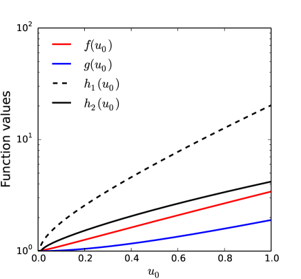
Figure 1: Functional forms of $f(u_{0})$ (defined as Equation (36)), $g(u_{0})$ (defined as Equation (53)), $h_{1}(u_{0})$ (defined as Equation (57)), and $u_{2}(u_{0})$ (defined as Equation (59)) in the range $0<u_{0}<1$.

In principle, $t_{\rm E}$ cannot be known perfectly from WFIRST for two reasons. First, WFIRST observations are not perfect, so the associated $t_{\rm E}$ measurement has a statistical uncertainty $\sigma_{\rm W}(t_{\rm E})$. Second, even if $t_{\rm E}$ from WFIRST can be constrained extremely precisely, $t_{\rm E}$ of the same event as seen from Earth is still uncertain to a limited level $\Delta t_{\rm E}$, due to the relative velocity between WFIRST and Earth. However, as we show in Appendix A, $t_{\rm E}$ for ground-based observations can be treated as “perfectly” known as long as the uncertainty in $t_{\rm E}$ inferred from WFIRST is smaller, by a certain specified factor (Equation (64)), than the uncertainty in $t_{\rm E}$ from ground-based observations. We have further proved in Appendices A and B that this condition is almost always satisfied for both the WFIRST statistical uncertainty $\sigma_{\rm W}(t_{\rm E})$ and the WFIRST-Earth systematic offset $\Delta t_{\rm E}$.

Therefore, the assumption that $t_{\rm E}$ is perfectly known from WFIRST almost always holds, so that $\sigma_{2}(t_{\rm eff})$ is mostly what we can get for the uncertainty in $t_{\rm eff}$ from ground-based observations.

Equations (21) and (22) have a number of important implications. First, the two terms entering $\Lambda$ have exactly the same errors in the high magnification limit, namely $\sqrt{8t_{\rm eff}/\pi\Gamma}\sigma_{0}/F_{\rm peak}$. Second, the errors scale strongly with magnification, $\propto u_{0}^{3/2}$ times the correction factor. This implies a strong magnification bias, so that the much more numerous faint potential sources can relatively easily enter the sample at high magnification. The magnification bias is stronger for $\sigma(t_{\rm eff})$ than for $\sigma(t_{0})$, suggesting that $\pi_{{\rm E},\parallel}$ is always better determined than $\pi_{{\rm E},\perp}$. However, comparison of $g(u_{0})$ and $h_{2}(u_{0})$ shows that this superiority is relatively modest.

Third, $t_{0}$ is not correlated with other parameters, and in particular it is not correlated with $t_{\rm eff}$. This is simply due to the fact that $\partial F/\partial t_{0}$ is an odd function of $t$, while the other derivatives are even in $t$. This is true for both Equations (14) and (18).

Fourth, $t_{\rm eff}$ is correlated with other parameters. As the first indication of why this is important, we note that even in the high-magnification limit, $t_{\rm eff}$ remains significantly correlated with $F_{\rm peak}$ (correlation coefficient $-\sqrt{2/3}$). Hence, for example, if there were independent information about the source flux, the error in $t_{\rm eff}$ could be reduced by a factor up to $\sqrt{3}$.

To make a quantitative estimate of the microlens parallax errors, we adopt parameters typical of KMTNet. We assume $\Gamma_{\oplus}=240\,{\rm day}^{-1}$, i.e., one observation per 2 minutes, for four hours per night (which is the time the Bulge is visible at the midpoint of the WFIRST campaigns) at each of three observatories, and 33% bad weather. We normalize the errors to 0.05 magnitudes at $I=18$. We then find

$$\left[\begin{array}[]{c}\sigma(\pi_{{\rm E},\parallel})\cr\sigma(\pi_{{\rm E},\perp})\end{array}\right]=\frac{0.52}{\cos\psi}\,\left(\frac{t_{\rm E}}{\rm day}\right)^{-1/2}10^{\frac{I_{s}-18}{2.5}}u_{0}^{3/2}\left[\begin{array}[]{c}g(u_{0})\cr h_{2}(u_{0})\end{array}\right]\ .$$ (23)

where $\psi$ is the phase of the WFIRST orbit relative to quadrature at the peak of the event. We note that because the observations are centered at quadrature, $0.82\leq\cos\psi\leq 1$. At first sight this pre-factor does not look especially promising, particularly given the fact that typical WFIRST microlensing sources will be substantially fainter than $I_{s}=18$. However, there are three points to keep in mind. First, we expect $t_{\rm E}\sim 1\,$day events to correspond to $M\sim M_{\rm Jup}$ lenses, whose parallaxes would be $\pi_{\rm E}\sim 4$ if they lay in the disk and $\pi_{\rm E}\sim 1.5$ in the bulge. Second, 10% of a “fair sample” of events will have $u_{0}<0.1$ and so errors that are $\gtrsim 30$ times smaller. Third, the sample of events will not be “fair”, but rather heavily biased toward fainter sources at high-magnification.

Regarding the first point, in order to make clear the measurability of parallax, it is better to express Equation (23) in terms of $\Lambda$, since this is a purely kinematic variable that does not vary with the lens mass

$$\left[\begin{array}[]{c}\sigma(\Lambda_{\parallel})\cr\sigma(\Lambda_{\perp})\end{array}\right]=\frac{0.30\sec\psi}{1000\,{\rm km~{}s^{-1}}}\,\left(\frac{t_{\rm E}}{\rm day}\right)^{1/2}10^{\frac{I_{s}-18}{2.5}}u_{0}^{3/2}\left[\begin{array}[]{c}g(u_{0})\cr h_{2}(u_{0})\end{array}\right]\ .$$ (24)

This shows that WFIRST-Earth parallaxes become more sensitive at shorter timescales (at fixed $\Lambda$ or projected velocity $\tilde{v}$).

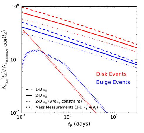
Figure 2: The normalized numbers of events with 1-D parallax ($\pi_{{\rm E},\parallel}$) and 2-D parallax ($\mbox{\boldmath$\pi$}_{\rm E}$) measured better than 5-$\sigma$ for two sets of typical events, respectively. For “Disk events”, we adopt $\pi_{\rm rel}=0.12$ mas and $\mu=7~{}{\rm mas}\,{\rm yr}^{-1}$, and for “Bulge events”, we adopt $\pi_{\rm rel}=0.02$ mas and $\mu=4~{}{\rm mas}\,{\rm yr}^{-1}$. For each set of typical events, we show two curves for the 2-D parallax measurements, one with perfect $t_{\rm E}$ information from WFIRST (solid lines) and the other without any external $t_{\rm E}$ information (dash-dotted lines). The former is more realistic (see Section 3). We also show the number of events for which there are both ${\mbox{\boldmath$\pi$}}_{\rm E}$ measurements and $\theta_{\rm E}$ measurements (from finite source effects), as discussed in Section 5.3. The normalization is the number of events with WFIRST baseline photometric precision better than 1%, which corresponds to a baseline magnitude of $H=20.2$ (Gould, 2014b). We assume the WFIRST microlensing sources follow the luminosity function of Bulge stars derived by Holtzman et al. (1998).

We illustrate this sensitivity in Figure 2 by showing the number of events that satisfy $\pi_{\rm E}/\sigma(\pi_{{\rm E},\parallel})>5$ (or $\pi_{\rm E}/\sigma(\pi_{{\rm E},\perp})>5$) for typical Bulge lenses ($\tilde{v}={\rm AU}\mu_{\rm rel}/\pi_{\rm rel}=1000\,{\rm km~{}s^{-1}}$) and typical disk lenses ($\tilde{v}=280\,{\rm km~{}s^{-1}}$). Here we have assumed $A_{I}=1.5$ and then integrated over the Holtzman et al. (1998) luminosity function. The Figure is normalized to the number of events with WFIRST baseline photometric precision better than 1%. This number can in turn be estimated for any specific WFIRST strategy that is either considered or adopted, and of course can be empirically determined from the experiment itself.

There are several important points regarding Figure 2. First, by incorporating the $t_{\rm E}$ information from WFIRST observations, we are able to increase the number of 2-D parallax detections by a factor $\sim$1.2. Second, the full parallax ($\mbox{\boldmath$\pi$}_{\rm E}$) curves with and without incorporating $t_{\rm E}$ information from WFIRST lie only about a factor of 1.2 and 1.5 below the $\pi_{{\rm E},\parallel}$ curves, respectively, despite the more serious deteriorations of $h_{i}(u_{0})$ relative to $g(u_{0})$ shown in Figure 1. This is because first the measurements are dominated by events with relatively low $u_{0}\lesssim 0.2$ for which the average ratio $\langle h_{1}(u_{0})/g(u_{0})\rangle<2$, and second, for a given source star, this can be compensated by going lower in $u_{0}$ by a factor $2^{2/3}=1.6$.

Figure 2 also shows that the 2-D parallax measurements will be available for a substantial fraction of Jupiter-mass FFPs ($t_{\rm E}\lesssim 1\,$day) in the disk and for Earth-mass FFPs ($t_{\rm E}\lesssim 0.05\,$day) in the Bulge. Shorter events are in general preferred, but the WFIRST-Earth parallax method implicitly sets a lower limit on the event timescale $t_{\rm E}$ that it can probe. This is because the same event must be observable from both WFIRSTand Earth, so that ${\rm AU}/\pi_{\rm E}\gtrsim D_{{\rm sat},\perp}$, or

$$t_{\rm E}\gtrsim 0.02~{}{\rm day}~{}\left(\frac{\tilde{v}}{10^{3}~{}{\rm km~{}s^{-1}}}\right)^{-1}\cos\psi\ .$$ (25)

Therefore, Equations (23) and (24) are only valid for disk events with $t_{\rm E}\gtrsim 0.06$ days and Bulge events with $t_{\rm E}\gtrsim 0.02$ days.

4 One-Dimensional Parallaxes

We now focus attention on 1-D parallaxes. As just mentioned, these can be measured about 1.2 to 1.5 times more frequently than 2-D parallaxes by comparing WFIRST and ground-based lightcurves. However, our primary reason for this focus is that WFIRST can, by itself measure 1-D parallaxes for sufficiently long events. That is, WFIRST-Earth and WFIRST-only measurements are complementary, being respectively most sensitive in the short $t_{\rm E}$ and long $t_{\rm E}$ regimes.

Of course, the main disadvantage of 1-D parallaxes is that they appear to be of little practical value. We will show, however, that this assessment is far too pessimistic.

4.1 WFIRST-only 1-D Parallaxes

We begin by making an estimate of the WFIRST-only 1-D parallax errors via Fisher matrix. Because WFIRST is observing near quadrature, it is accelerating transverse to the line of sight at

$$a_{\perp}\simeq{\rm AU}\Omega_{\oplus}^{2}\cos\psi;\qquad\psi\equiv\Omega_{\oplus}(t-t_{\rm quad}).$$ (26)

Here $\Omega_{\oplus}\equiv 2\pi/$yr and $t_{\rm quad}$ is the epoch when the field is at quadrature. In the approximation that the acceleration is constant, this induces a quadratic deviation in the lightcurve, which to lowest order implies a normalized lens-source separation $u(t)$,

$$[u(t)]^{2}=\biggl{[}{t-t_{0}\over t_{\rm E}}+{1\over 2}\pi_{{\rm E},\parallel}(\Omega_{\oplus}(t-t_{0}))^{2}\cos\psi\biggr{]}^{2}+u_{0}^{2}\ .$$ (27)

This leads to an asymmetric distortion in the magnification (Gould et al., 1994). With this as well as Equation (11), one finds that

$$\frac{\partial F}{\partial\pi_{{\rm E},\parallel}}=\frac{F_{\rm s}\Omega_{\oplus}^{2}t_{\rm E}^{2}\cos\psi}{2}\frac{A^{\prime}\tau^{3}}{u}\qquad(\pi_{{\rm E},\parallel}\ll 1)\ .$$ (28)

Because Equation (28) is odd in $t$, the only other microlensing parameter that it couples to is $t_{0}$. Thus, the Fisher matrix is two-dimensional. To evaluate this, we first specify that WFIRST observations will generally be above sky, so that the flux errors scale $\sigma=\sigma_{0,{\rm W}}A^{1/2}$, where $\sigma_{0,{\rm W}}$ is the error at baseline. As in Equation (13), we approximate the observations as being at a uniform rate $\Gamma_{\rm W}$, and find

$$b_{ij} = \frac{\Gamma_{\rm W}t_{\rm E}}{\sigma_{0,{\rm W}}^{2}}\int\frac{\partial F}{\partial a_{i}}\frac{\partial F}{\partial a_{j}}\frac{d\tau}{A}$$ (29)

$$= \frac{\Gamma_{\rm W}F_{\rm s}^{2}}{4\sigma_{0,{\rm W}}^{2}t_{\rm E}}\left(\begin{array}[]{cc}4G_{0}&-2\eta G_{1}\cr-2\eta G_{1}&\eta^{2}G_{2}\end{array}\right)\ ,$$ (32)

where $\eta\equiv\Omega_{\oplus}^{2}t_{\rm E}^{3}\cos\psi$, and

$$\left\{\begin{array}[]{rcl}G_{0}&\equiv&\int A^{\prime 2}A^{-1}u^{-2}\tau^{2}d\tau\cr G_{1}&\equiv&\int A^{\prime 2}A^{-1}u^{-2}\tau^{4}d\tau\cr G_{2}&\equiv&\int A^{\prime 2}A^{-1}u^{-2}\tau^{6}d\tau\end{array}\right.\ .$$ (33)

Then the covariance matrix is

$$c_{ij}=b_{ij}^{-1}=\frac{\sigma_{0,{\rm W}}^{2}t_{\rm E}}{\Gamma_{\rm W}F_{\rm s}^{2}\eta^{2}}\frac{1}{G_{0}G_{2}-G_{1}^{2}}\left(\begin{array}[]{cc}\eta^{2}G_{2}&2\eta G_{1}\cr 2\eta G_{1}&4G_{0}\end{array}\right)\ .$$ (34)

The uncertainty in $\pi_{{\rm E},\parallel}$ is given by $\sigma(\pi_{{\rm E},\parallel})=c_{22}^{1/2}$. It can be expressed analytically only in the high magnification limit. Therefore, similarly to the case of WFIRST+ground 2-D parallaxes, we introduce a correction factor $f(u_{0})$ that approaches unity as $u_{0}$ approaches zero, and rewrite $\sigma(\pi_{{\rm E},\parallel})$ as

$$\sigma(\pi_{{\rm E},\parallel})=1.77\frac{\sigma_{0,{\rm W}}}{F_{\rm s}}\frac{\sec\psi}{\Omega_{\oplus}^{2}t_{\rm E}^{5/2}\Gamma_{\rm W}^{1/2}}f(u_{0})\ ,$$ (35)

where $1.77=[14/3-32^{1/2}\ln(1+\sqrt{2})]^{-1/2}$ is the result of an analytic calculation, and

$$f(u_{0})\equiv 1.13\sqrt{\frac{G_{0}}{G_{0}G_{2}-G_{1}^{2}}}\ .$$ (36)

This function is also illustrated in Figure 1. The deterioration toward higher $u_{0}$ is primarily due to the fact that the high-mag peak contributes the majority of the information about $\pi_{{\rm E},\parallel}$. Secondarily, $t_{0}$ becomes increasingly correlated with $\pi_{{\rm E},\parallel}$ at higher $u_{0}$.

Adopting a cadence of $\Gamma_{\rm W}=100~{}{\rm day}^{-1}$ and assuming 0.01 mag errors at $H=20.2$ (Gould, 2014b), this yields

$$\sigma(\pi_{{\rm E},\parallel})=\frac{0.017}{\cos\psi}10^{\frac{H_{\rm s}-20}{5}}\left({t_{\rm E}\over 10\,\rm day}\right)^{-5/2}f(u_{0})\ .$$ (37)

For an intuitive understanding of the relevance of this error bar to the parallax measurement, it is best to express it in terms of $\Lambda_{\parallel}$

$$\sigma(\Lambda_{\parallel})={0.10\,\sec\psi\over 1000\,{\rm km~{}s^{-1}}}10^{\frac{H_{s}-20}{5}}\biggl{(}{t_{\rm E}\over 10\,\rm day}\biggr{)}^{-3/2}f(u_{0})\ .$$ (38)

From Equations (37) and (38), it is clear that WFIRST will make very good $\pi_{{\rm E},\parallel}$ measurements for long events but will do much worse for short events. For example, for $t_{\rm E}=2$ days, the pre-factor in Equation (38), goes from 0.10 to 1.1.

4.2 Combined Orbital and Two-Observatory 1-D Parallaxes

Comparison of Equations (24) and (38) shows that the two approaches to obtaining 1-D parallaxes are complementary, with precisions $\sigma(\Lambda_{\parallel})\propto t_{\rm E}^{1/2}$ for WFIRST-Earth parallaxes and $\sigma(\Lambda_{\parallel})\propto t_{\rm E}^{-3/2}$ for WFIRST-only parallaxes. The normalizations ($I_{S}=18$ in the first and $H_{s}=20$ in the second) may appear deceptive, particularly because typical sources will have $(I-H)\sim 0.8+E(I-H)\sim 1.8$ assuming $E(I-H)\sim 1$. However, one must bear in mind that that the two-observatory formula has a very strong dependence on $u_{0}$, whereas the WFIRST-only formula is, by comparison, almost flat in $u_{0}$.

To investigate this further, we consider the combined impact of both measurements, assuming $A_{H}=0.5$ and (as before) a Holtzman et al. (1998) luminosity function and $A_{I}=1.5$. We denote the precision derived by combining these two formulae by $\sigma_{\rm full}(\pi_{{\rm E},\parallel})$.

We show in Figure 3 the numbers of events with 1-D parallax measurements better than a specified (absolute and relative) precision for WFIRST-only and WFIRST plus ground observations, respectively. The normalizations are again to the number of events with WFIRST baseline precisions of 1%. Figure 3 demonstrates the importance of ground-based observations in measuring 1-D parallaxes: without these observations, WFIRST will not be able to make any meaningful 1-D parallax measurements for short timescale events.

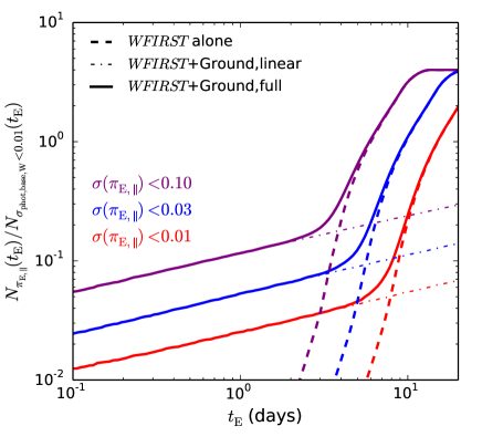
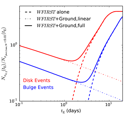
Figure 3: The normalized numbers of events with 1-D parallax ($\pi_{{\rm E},\parallel}$) measurements better than given precisions for WFIRST-only observations (dashed lines), WFIRST plus ground-based survey observations (dash-dotted lines for linear approximation and solid lines for full derivation). The left panel shows curves with absolute measurement uncertainties ($\sigma(\pi_{{\rm E},\parallel})$). The right panel shows curves with 5-$\sigma$ detections ($\pi_{{\rm E},\parallel}/\sigma(\pi_{{\rm E},\parallel})=5$) for typical disk events ($\pi_{\rm rel}=0.12$ mas, $\mu=7~{}{\rm mas}\,{\rm yr}^{-1}$) and Bulge events ($\pi_{\rm rel}=0.02$ mas, $\mu=4~{}{\rm mas}\,{\rm yr}^{-1}$). The normalization is the same as that used in Figure 2. That is, the number of events with WFIRST baseline photometric precision seen by WFIRST better than 1%. The flattening for $t_{\rm E}>10$ days is caused by our restriction that $u_{0}\leq 1$, but it is very likely real for two reasons. First, $\pi_{{\rm E},\parallel}$ measurements will be quite difficult for $u_{0}>1$, as the correlation between $t_{0}$ and $\pi_{{\rm E},\parallel}$ becomes significant (correlation coefficient $r(t_{0},\pi_{{\rm E},\parallel})\geq 0.65$ for $u_{0}\geq 1$); and second, many events with $t_{\rm E}>10$ days will not be fully covered by WFIRST observations.

4.3 Xallarap and Lens Orbital Motion

Measurements of ${\mbox{\boldmath$\pi$}}_{\rm E}$ made from a single observatory can be corrupted by xallarap (motion of the source about a companion) and lens orbital motion (motion of the lens about a companion), whereas those derived from comparison of contemporaneous measurements from two observatories cannot. This is because the basis of single-observatory ${\mbox{\boldmath$\pi$}}_{\rm E}$ measurements is the accelerated motion of the observer, which can in principle be perfectly mimicked by accelerated motion of the source (or the lens). Below we only consider the acceleration of the source (i.e., xallarap effect), but our methodology applies to the other case as well.

In the case of complete 2-D ${\mbox{\boldmath$\pi$}}_{\rm E}$ measurements, xallarap-dominated acceleration effects can in principle be distinguished from the parallax effects from their orbital period and the direction of their implied angular momentum vector. That is, if the effects of parallax are mistakenly attributed to xallarap, then the xallarap solution will lead to a companion with a 1-year period and orbital axis that is exactly aligned to that of the Earth’s (projected on the plane of the sky) (Poindexter et al., 2005).

This purely internal test fails completely, however, for 1-D parallaxes, unless the period is so short that a 2-D xallarap solution can be reliably extracted from the data. The contamination of 1-D parallaxes due to xallarap has never previously been estimated, probably due to the limited previous interest in 1-D parallaxes themselves.

The contamination due to xallarap can be rigorously calculated under the assumption that the multiplicity properties (masses and semi-major axes) of companions to the microlensed sources are similar to those of solar-type stars in the solar neighborhood. We first note that the amplitude of Earth’s acceleration relative to the projected Einstein radius $\tilde{r}_{\rm E}\equiv{\rm AU}/\pi_{\rm E}$ is (at quadrature) $\tilde{A}=(GM_{\odot}/{\rm AU}^{2})/\tilde{r}_{\rm E}$. The component of this acceleration entering $\pi_{{\rm E},\parallel}$ is $\tilde{A}\cos\phi_{\pi}$.

By the same token, the acceleration due to a companion of mass $m$ and semi-major axis $a$ relative to the Einstein radius projected on the source plane $\hat{r}_{\rm E}\equiv D_{\rm S}\theta_{\rm E}$, is $\hat{A}=(Gm/a^{2})/\hat{r}_{\rm E}$. And the component that contributes to the asymmetry of the event is $\hat{A}\cos\phi_{\xi}$, where $\phi_{\xi}$ is the angle between the lens-source relative motion and the instantaneous acceleration of the source about its companion. Hence, the ratio of the xallarap-to-parallax signals contributing to this asymmetry is

$${|\xi_{\parallel}|\over|\pi_{{\rm E},\parallel}|}={\hat{A}|\cos\phi_{\xi}|\over\tilde{A}|\cos\phi_{\pi}|}={m\over M_{\odot}}\,\biggl{(}{a\over{\rm AU}}\biggr{)}^{-2}{D_{\rm L}\over D_{\rm LS}}{|\cos\phi_{\xi}|\over|\cos\phi_{\pi}|},$$ (39)

where $D_{\rm LS}\equiv D_{\rm S}-D_{\rm L}$ is the distance between the lens and the source.

To evaluate the distribution of this ratio for Bulge lenses, we first adopt $D_{\rm L}/D_{\rm LS}=8$. We then consider the ensemble of binary companions in Figure 11 of Raghavan et al. (2010), which is a complete sample of companions for 454 G-dwarf primaries. We restrict attention to the 53 companions with semi-major axes $0.2<a/{\rm AU}<30$ on the grounds that the handful of closer companions would be recognized as such from oscillations in the lightcurve, while those farther away would induce asymmetries that are too small to measure. We allow $\phi_{\pi}$ to vary randomly over a circle and $\phi_{\xi}$ to vary randomly over a sphere. Figure 4 shows that xallarap contamination is very serious ($>$100%) for about 2% of Bulge lenses and is significant ($>$10%) for about 4.5%. In addition, we note that there is a comparable contamination from the acceleration of the lenses due to their companions (both with and without binary lightcurve signatures).

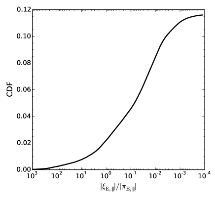
Figure 4: The fraction of Bulge events ($D_{\rm L}/D_{\rm LS}=8$) with parallax signal affected by the xallarap effect to a given precision.

Therefore, with WFIRST alone up to 9% of all events will show false parallax detections. Such contamination would be removed by a complementary ground-based survey for relatively short events ($t_{\rm E}\lesssim 3$ days). For longer events, this contamination cannot be removed completely due to the limited power of WFIRST-Earth 1-D parallax, but the study of this contamination in the short event sample allows to better interpret the 1-D parallax measurements for these longer events.

4.4 Value of $\pi_{{\rm E},\parallel}$ Measurements

A large sample of 1-D parallaxes with well-understood selection has two major uses. First, it can be directly analyzed to simultaneously derive a Galactic model and the lens mass function. Second, it allows one to derive the complete solution (namely individual masses, distances and transverse velocities) once combined with the measurement of the lens-source relative proper motion ${\mbox{\boldmath$\mu$}}_{\rm rel}$, which can be obtained for some events with WFIRST alone and even more events with follow-up imaging. These two applications are discussed in turn.

In both cases, we show that the addition of short $t_{\rm E}$ events from combining ground and space observations will play a critical role in understanding the low-mass end of the mass spectrum, i.e., brown dwarfs (BDs) and FFPs.

4.4.1 Statistical Studies Using 1-D Parallax Samples

At present, large microlensing samples with well-understood selection are characterized by a single microlensing variable, the Einstein timescale $t_{\rm E}$, i.e., no parallax information. Although not usually thought of this way, we dub this case as a “0-D parallax measurement” in order to contrast it to 1-D and 2-D parallaxes. That is, in the three cases, the available information consists of $(t_{E})$, $(t_{E},\pi_{{\rm E},\parallel})$, $(t_{E},\pi_{{\rm E},\parallel},\pi_{{\rm E},\perp})$.

The statistical interpretation of a 0-D parallax sample requires a Galactic model to constrain six of the input variables (lens and source distances and transverse velocities) to obtain information about the seventh (lens mass function). This situation is not as bad as it may first seem. The three source properties are well understood statistically from direct observations, even if these source properties are not measured for each individual event, and Galactic models are constructed based on a wide variety of very good data. Sumi et al. (2011) used this technique to infer the existence of a population of FFPs. Nevertheless, uncertainties in Galactic models remain considerable, and hence it would be valuable if microlensing studies could further constrain them rather than propagating them. Moreover, even if the Galactic model were known perfectly, the statistical precision of microlensing studies is greatly reduced by the requirement of deconvolving three parameters to learn about the one of greatest interest.

Han & Gould (1995) argued that individual lens mass and distance would be much more tightly constrained by measuring the full parallax vector ${\mbox{\boldmath$\pi$}}_{\rm E}$ in addition to $t_{\rm E}$, and Calchi Novati et al. (2015) showed that this was in fact the case for their sample of microlenses with Spitzer parallaxes. Their work still incorporated Galactic models, but the mass/distance constraints were dramatically improved compared the case with timescales alone. See also Gould (2000).

The 0-D parallaxes of Sumi et al. (2011) and the 2-D parallaxes of Calchi Novati et al. (2015) have had different applications. Specifically, the great value of the first is that it could make statistical statements about low-mass objects, while that of the second was the greatly improved precision of individual lenses. In particular, the 2-D study could not make any statement about low-mass objects because the Spitzer sample was strongly biased against short events.

For WFIRST 1-D parallaxes, the situation is clearly intermediate between the 0-D parallaxes of Sumi et al. (2011) and the 2-D parallaxes of Calchi Novati et al. (2015). The great potential value of WFIRST 1-D parallaxes (i.e., much stronger statistical statement about BDs and FFPs) would be almost completely lost if these substellar objects were systematically excluded from the 1-D parallax sample. Given the $\sigma(\Lambda_{\parallel})\propto t_{\rm E}^{-3/2}$ behavior of Equation (38) (also see Figure 3), this is exactly what would happen in the absence of a ground-based complementary survey. The addition of such a survey would enable 1-D parallax measurements across the entire range of timescale $t_{\rm E}\gtrsim 2\,$hrs for disk lenses.

4.4.2 Complete Solutions From $\pi_{{\rm E},\parallel}$ Plus ${\mbox{\boldmath$\mu$}}_{\rm rel}$

A complete solution of the lens (or the lens system) can be derived by combining the $\pi_{{\rm E},\parallel}$ measurement from the light curve and the ${\mbox{\boldmath$\mu$}}_{\rm rel}$ measurement from high-resolution imaging (Ghosh et al., 2004; Gould, 2014a), based on the definition of $t_{\rm E}$ (Equation (1)) and the fact that ${\mbox{\boldmath$\pi$}}_{\rm E}$ and ${\mbox{\boldmath$\mu$}}_{\rm rel}$ are along the same direction.

The measurement of ${\mbox{\boldmath$\mu$}}_{\rm rel}$ can be done by WFIRST alone, using its $\sim$40,000 high-resolution images, for relatively luminous ($\gtrsim$ early M-dwarfs) lenses (Bennett et al., 2007). Late-time high-resolution follow-up imaging can extend the domain of coverage to all luminous lenses (i.e., $M>0.08\,M_{\odot}$) and can also improve the precision, as well as resolving certain ambiguities that we discuss in Section 4.3. Such imaging has already achieved important results using HST (Alcock et al., 2001; Bennett et al., 2015) and Keck (Batista et al., 2015), but will potentially be much more powerful using next generation telescopes (Gould, 2014a; Henderson, 2015)

Before proceeding, one may ask why one would need microlensing mass and distance measurements for a (subsequently) resolved lens, since photometric estimates would then be available. As pointed out by Gould (2014a), the answer is two-fold. First, one would always prefer measurements to estimates. Second, high-resolution imaging alone may not identify the correct microlenses. Because roughly 2/3 of all stars are in binaries, and since the lensing cross section scales as $\theta_{\rm E}\propto M^{1/2}$, of order 1/3 of the events due to binaries will in fact be generated by the lower-mass (and generally fainter) companion. In the majority of such cases, the star that actually generated the event will not be visible, because it is either unresolved or dark. Hence, for tens of percent of cases, the lens would be misidentified by such simple imaging. Gould (2014a) shows how these cases can be identified and resolved by a combination of 1-D parallaxes and imaging.

A large homogeneous sample of events with both $\pi_{{\rm E},\parallel}$ and ${\mbox{\boldmath$\mu$}}_{\rm rel}$ measurements has several benefits. First, it would permit one to derive a Galactic model (rather than assuming one). Second, it would permit one to measure the lens mass function over the range of masses that are probed. Third, for all the planetary events in this sample, one would gain a precise mass measurement of the host and thus (in almost all cases) of the planet.

Even without a complementary ground-based survey, all of these benefits could be derived at least partially from WFIRST observations themselves. However, these observations alone would probe only the upper half or so of the mass function, partly because WFIRST-only 1-D parallax measurements require long-timescale events, and partly because WFIRST proper motion measurements require luminous lenses. Similarly, the masses of planets orbiting low-mass hosts would remain undetermined.

Hence, complementary ground-based survey observations are crucial to probe the low-mass stellar and substellar lenses.

4.5 Value of ${\mbox{\boldmath$\pi$}}_{\rm E}$ Measurements

As discussed following Equation (24), the 2-D parallax measurements are biased toward substellar objects. These are exactly the objects that are inaccessible to the conversion of 1-D parallaxes to complete solutions that was discussed in Section 4.4.2. These 2-D parallax measurements enable us to directly derive the complete solutions purely from the microlensing light curves for the roughly 50% of all planetary and binary events in which $\theta_{\rm E}$ can be measured (Zhu et al., 2014). See Section 6 for details. While most of these 2-D parallax measurements in single-lens events will not yield complete solutions (but see Section 5), Calchi Novati et al. (2015) have shown that 2-D parallax measurements, when combined with a Galactic model, give tight constraints on mass and distance, particularly for disk lenses. This is important not only to further constrain the substellar mass function relative to the analysis that is possible based on 1-D parallaxes (Section 4.4.1), but also for a more detailed understanding of individual objects.

5 Einstein Radius Measurements: $\theta_{\rm E}$

The particular interest of the $\theta_{\rm E}$ measurement is that if there is also a measurement of ${\mbox{\boldmath$\pi$}}_{\rm E}$, then it yields a complete solution (i.e., mass, distance and transverse velocity).

5.1 WFIRST-only Einstein-Radius Measurements

In the case of single-lens events, if the lens transits the source, then the light curve is distorted by the finite source effect, which yields $\rho\equiv\theta_{*}/\theta_{\rm E}$, the ratio of the source radius to the angular Einstein radius. Because $\theta_{*}$ can be determined from the dereddened color and magnitude of the source (Yoo et al., 2004), this yields a measurement of $\theta_{\rm E}$ and so also of the proper motion $\mu_{\rm rel}=\theta_{\rm E}/t_{\rm E}$ (Gould, 1994a). Such transits occur with probability $\sim\rho$, which is typically of order $\sim 3\times 10^{-3}$ for main-sequence sources and and $\sim 3\times 10^{-2}$ for giant sources.

When the observational bias is taken into account, the number of single-lens events with finite-source effects should be more than what one would naively estimate based purely on the above transit probability. Single-lens events with finite-source effects can reach extremely high magnifications, so they can be detected even though the source stars at baseline are extremely faint. For example, an M6 dwarf in the Bulge has $H=26$ (assuming an extinction of $A_{H}=0.5$) and an angular radius $\theta_{\star}=0.06\mu$as, and can be magnified in brightness by $A_{\rm max}=2/\rho$ when a lens transits exactly through its center. For a Neptune-mass Bulge lens, this event will reach $H=21$ at its peak. WFIRST can therefore obtain on average one observation during the entire transit with a photometric precision of 1.4%, which would yield a precise measurement of $\rho$. Hence if the lens is more massive than Neptune, then essentially all luminous stars in the Bulge can serve as source stars for events with measurable finite-source effects. For Earth-mass Bulge lenses, 2% precision can be reached for individual measurements of M4 ($M\sim 0.25\,M_{\odot}$, $R\sim 0.25\,R_{\odot}$) sources, yielding similar quality $\theta_{\rm E}$ determinations (since there are on average 2 measurements per transit). Therefore, although small stars are disfavored by their small angular size, they contribute more significantly to the number of single-lens events with finite-source effects, than they do to the number of all detectable single-lens events.

5.2 WFIRST+Ground Einstein-Radius Measurements

In this subsection, we wish to understand how the addition of a ground-based network contributes to the frequency of such measurements. The answer is: quite modestly. There are two issues. First, an aggressive ground-based network will only observe the WFIRST field about half the time. Since the source crossings typically last only about 1–2 hours, it is this instantaneous coverage that matters rather than daily coverage. Second, if the source size, projected on the observer plane ($\rho{\rm AU}/\pi_{\rm E}$) is larger than the Earth-satellite projected separation $D_{{\rm sat},\perp}$, then the probability that the source will transit at least one of the two observers is not substantially increased. That is, if the ground observatory is taking observations at the time of the peak, it can roughly double this probability provided that

$${\rho{\rm AU}\over\pi_{\rm E}D_{{\rm sat},\perp}}=100{\theta_{*}\over\pi_{\rm rel}}\sec{\psi}<1.$$ (40)

That is,

$$\pi_{\rm rel}>60\,{\mu\rm as}\biggl{(}{\theta_{*}\over 0.6\,{\mu\rm as}}\biggr{)}^{-1}\sec{\psi}\ ,$$ (41)

where we have normalized to the angular radius of a typical solar-type source. Thus, for main sequence sources, the simultaneous ground-based observations contribute $\theta_{\rm E}$ measurements for disk lenses but not Bulge lenses. The situation is even less favorable for sub-giant and giant sources, which are a small minority of all sources but a larger fraction of all finite-source events due to their larger size (Zhu et al., 2015b). In brief, we expect that the ground-based survey will add only 10–20% to the rate of $\theta_{\rm E}$ measurements. This is small enough to ignore for present purposes.

5.3 Value of $\theta_{\rm E}$ Measurements

The main value of $\theta_{\rm E}$ measurements, which come primarily from WFIRST observations alone, is derived from combining them with the vector ${\mbox{\boldmath$\pi$}}_{\rm E}$ measurements, which come primarily from combining WFIRST and ground-based survey data. We therefore evaluate the conditional probability that $\theta_{\rm E}$ is measurable given that ${\mbox{\boldmath$\pi$}}_{\rm E}$ is measured.

The impact parameter as seen from Earth, $u_{0,\oplus}$, that would allow for a $\mbox{\boldmath$\pi$}_{\rm E}$ measurement is limited by

$$(S/N)_{\rm th}\leq\frac{\pi_{\rm E}}{\sigma(\pi_{{\rm E},\perp})}=\frac{\Lambda D_{{\rm sat},\perp}}{\sigma_{2}(t_{\rm eff})}\ ,$$ (42)

where $(S/N)_{\rm th}$ is the threshold for claiming a reliable detection. By approximating $u_{0}^{3/2}h_{2}(u_{0})\propto u_{0}^{\alpha}$ ($\alpha\approx 1.7$) in Equation (22), we can derive the maximum allowed impact parameter $u_{0,\oplus,{\rm max}}$

$$u_{0,\oplus,{\rm max}}\propto\left(\frac{\Lambda D_{{\rm sat},\perp}}{(S/N)_{\rm th}}\right)^{1/\alpha}\left(\frac{F_{\rm s}}{\sigma_{0}}\right)^{1/\alpha}\left(\frac{\Gamma_{\oplus}}{t_{\rm E}}\right)^{1/(2\alpha)}\ .$$ (43)

The impact parameter as seen from WFIRST is given by $u_{0,{\rm W}}=u_{0,\oplus}+\Delta u_{0}$, where $\Delta u_{0}$ is related to $\pi_{{\rm E},\perp}$ by Equation (4). For $0.1$ days$\leq t_{\rm E}\leq 3$ days and below sky sources as seen from Earth, one can easily prove that $\Delta u_{0}\lesssim u_{0,\oplus,{\rm max}}$, so that the maximum allowed impact parameter as seen from WFIRST, $u_{0,{\rm W},{\rm max}}$, is similar to $u_{0,\oplus,{\rm max}}$. Then the conditional probability can be estimated as

$$P=\frac{\rho}{u_{0,{\rm W},{\rm max}}}=\frac{\theta_{\star}}{\mu_{\rm rel}t_{\rm E}u_{0,{\rm W},{\rm max}}}\ .$$ (44)

The stellar angular radius $\theta_{\star}$ is also related to the stellar flux $F_{\rm s}$: $\theta_{\star}\propto F_{\rm s}^{\beta}$, and we take $\beta\approx 0.3$ as a reasonable value for $I$ band. By only keeping $F_{\rm s}$ and $t_{\rm E}$, we find

$$P\propto F_{\rm s}^{\beta-1/\alpha}~{}t_{\rm E}^{1/(2\alpha)-1}\approx F_{\rm s}^{-0.3}~{}t_{\rm E}^{-0.7}\ .$$ (45)

Hence, this conditional probability is only weakly dependent on source flux and has a substantially stronger dependence on Einstein timescale.

We adopt $\theta_{*}=0.15\,{\mu\rm as}\,10^{0.12(23.5-I_{0})}$ and use $\sigma_{2}(t_{\rm eff})\propto u_{0}^{3/2}h_{2}(u_{0})$ to evaluate $P$ numerically and show the results in Figure 2. In doing so, we do not count any events for which $P>1$, since this implies that the source is too big to permit high-enough magnification for $t_{\rm eff}$ to be measured. Figure 2 shows that complete mass measurements peak at roughly 0.2 days for Bulge lenses and 0.1 days for Disk lenses, where in both cases they constitute roughly half of the 2-D parallax measurements.

6 Complete Solutions for Binary and Planetary Events

Finally, although the complete solutions (${\mbox{\boldmath$\pi$}}_{\rm E}$ plus $\theta_{\rm E}$) for isolated stellar-mass lenses will be rare, such measurements are much more common for planetary and binary events, because roughly half of the recognizable such events will show steep features due to caustic crossings and cusp crossings. For these, measurement of $\theta_{\rm E}$ by WFIRST will be virtually automatic. Moreover, these events will also have greatly enhanced 2-D parallax measurements by three different channels.

First, An & Gould (2001) argued that caustic crossing events yield full 2-D parallaxes much more easily than events without sharp features (either single-lens events or non-caustic-crossing multiple lenses). The sharp features break the continuous degeneracies among the parameters that are even in $t$. They also break the symmetry of the lightcurve, which is the fundamental cause of the fourth-order time dependence of $\pi_{{\rm E},\perp}$ found by Smith et al. (2003) for single-lens events. While there has been no firm proof that this is the case, there is substantial circumstantial evidence from the high fraction of planetary lenses with well-determined parallaxes relative to single lens events of similar $(u_{0},t_{\rm E},f_{s})$. Hence, it is likely that WFIRST will by itself measure many 2-D parallaxes of caustic-crossing binary and planetary events, particularly for those with timescales $t_{\rm E}\gtrsim 7\,$days, for which the corresponding single-lens events show good 1-D parallax measurements. See Figure 3.

Second, events with two caustic crossings observed from both WFIRST and the ground can also yield 2-D parallax determinations based on two $\Delta t_{\rm cc}$ measurements, one at each crossing. Here $\Delta t_{\rm cc}$ is the difference of the caustic crossing time as seen from WFIRST and the ground. When they proposed the method of parallax observations of caustic crossings, Hardy & Walker (1995) already recognized that these yield only 1-D information because small displacements along the direct parallel to the caustic do not generate substantial changes in the lightcurve. This is in striking contrast to single lenses, for which displacements in both directions induce effects of the same order. See Figure 1. Graff & Gould (2002) pointed out that this problem could be solved if there were two caustic crossings (which is typical of most events, i.e., entrance and exit) provided that the caustics themselves are not approximately parallel. Zhu et al. (2015a) and Shvartzvald et al. (2015) showed in practice that binary events with only one $\Delta t_{\rm cc}$ measurement are subject to both discrete and continuous degeneracies.

One shortcoming of this approach with regard to WFIRST is that, given a network of three southern hemisphere telescopes, each caustic crossing can be observed from the ground with approximately 50% probability simply because the bulge is visible from each observatory only about 4 hours per night, averaged over the WFIRST campaign. This emphasizes the importance of having a network, but also of increasing it to as many independent locations as possible. For the example of the KMTNet network, adding a node in Hawaii would be valuable.

Yet a third channel would be to combine the WFIRST 1-D orbital parallax measurement with one $\Delta t_{\rm cc}$ measurement, for the case that there is only one, either because the second crossing was missed from the ground or because the geometry of the event only had one crossing (e.g., Shvartzvald et al. 2015). As in the previous approach there are constraints on the orientation of the caustic: it cannot be too close to perpendicular to $\hat{\bf n}$. This method may be the most frequently employed for shorter events, because, if the probability of catching a single crossing is $p=50\%$, then the ratio of one measured $\Delta t_{\rm cc}$ to two such measurements is $(2/p-1)\rightarrow 3$.

A full analysis of the measurability of such parallaxes lies well beyond the scope for the present work but we believe that this should be actively investigated.

7 Auxiliary Benefits of WFIRST Microlensing in Optical Fields

Complementary ground-based survey observations of the WFIRST microlensing fields have additional major benefits. First, ground-based surveys will be sensitive to planets in the wings of the events, in particular during the roughly 180 days (or 110 days) of a given year when WFIRST is not observing. Of course, the ground-based sensitivity to planets will be much lower than would be the case for WFIRST if it were observing. However, since it is not, this opens up completely new parameter space. While in some sense this parameter space is already available from ground-based surveys alone, the WFIRST sample is unique in its sensitivity to low mass planets. Hence, the addition of a ground-based survey would significantly enhance our understanding of the relation between the relatively close-in terrestrial planets that WFIRST is sensitive to and the more distant ice and gas giants that ground-based surveys are most sensitive to.

Second, it is likely that the characterization of microlensing sources and lenses (as well as other field stars) will benefit from follow-up observations, either individually or on a systematic basis. Such characterization is likely to benefit from the option of utilizing optical bands, and this would be greatly facilitated by observing low-to-moderate extinction fields.

8 Discussion

We propose here to augment the WFIRST microlensing campaigns with simultaneous observations from a ground-based network of wide-field survey telescopes, in order to 1) enable 1-D microlens parallax measurements over the entire mass range $M\gtrsim M_{\oplus}$, and 2) yield 2-D parallax measurements for a significant fraction of short-timescale $(t_{\rm E}\lesssim 3$ days) events and planetary/binary events. The 1-D parallax measurements can be used to produce complete solutions (mass, distance, transverse velocity) of the luminous lens systems ($M\gtrsim 0.08M_{\odot}$), once combined with the measurements of the lens-source relative proper motion ${\mbox{\boldmath$\mu$}}_{\rm rel}$ that come from WFIRST and/or ground-based follow-up high-resolution imaging. The 2-D parallax measurements will be especially useful for better understanding the substellar population. For the roughly 50% of planetary and binary events with caustic crossings, and for a significant fraction of FFP events, the angular Einstein radius $\theta_{\rm E}$ is also measured, and thus these 2-D parallax measurements directly lead to complete solution of the lens (or the lens system).

Our methodology applies as well to any other dedicated microlensing surveys that are conducted at L2, such as Euclid (Penny et al., 2013).

Because WFIRST launch is almost a decade in the future, one might in principle consider complementary observations from many different ground-based networks and/or individual telescopes. For example, one might consider a network of infrared and/or optical telescopes of various apertures and field sizes (e.g., similar to the ground-based network to support the K2 microlensing campaign, Henderson et al., 2015). Here, we have initiated such an investigation by considering an optical, KMTNet-like network, simply because these telescopes exist and it would not be trivial to build a new network with substantially greater capability. The KMTNet microlensing campaign is scheduled to last 5 years and thus is expected to end before the launch of WFIRST. Hence, coordination of KMTNet in particular with WFIRST would also require advance planning, and this is another reason to begin serious evaluation of the benefits of such complementary observations now.

At first sight, it might appear that KMTNet would be ill-matched to WFIRST. From the standpoint of finding planets, WFIRST will be vastly superior. However, the problem of augmenting WFIRST observations in order to measure parallaxes given a $\sim$0.01 AU displacement from WFIRST is far less challenging than finding planets from the ground. Hence, as we have shown (see, e.g., Figures 2 and 3), even 1.6m wide-field telescopes can yield excellent results for a very large fraction of events for which WFIRST is sensitive to planets, including FFPs. The WFIRST saturation magnitude might be another potential concern when complementing WFIRST with ground-based 1.6m telescopes. However, Gould et al. (2015) have shown this is not the case for near infrared cameras (see their Figure 1).

Appendix A Fisher Matrix Analysis for General Cases

The general point-lens point-source light curve is described by Equation (11). With this as well as Equations (12), (13), (14), and (15), the Fisher matrix can be evaluated

$$b_{ij}=\frac{\Gamma}{\sigma_{0}^{2}}\left(\begin{array}[]{cccc}t_{\rm E}^{-1}F_{\rm s}^{2}C_{0}&0&0&0\cr 0&t_{\rm E}u_{0}^{2}F_{\rm s}^{2}C_{1}&-u_{0}F_{\rm s}^{2}C_{0}&t_{\rm E}u_{0}F_{\rm s}C_{2}\cr 0&-u_{0}F_{\rm s}^{2}C_{0}&t_{\rm E}^{-1}F_{\rm s}^{2}C_{3}&-F_{\rm s}C_{4}\cr 0&t_{\rm E}u_{0}F_{\rm s}C_{2}&-F_{\rm s}C_{4}&t_{\rm E}C_{5}\cr\end{array}\right)\ ,$$ (46)

where

$$\left\{\begin{array}[]{rcl}C_{0}&\equiv&\int A^{\prime 2}\tau^{2}u^{-2}d\tau\cr C_{1}&\equiv&\int A^{\prime 2}u^{-2}d\tau\cr C_{2}&\equiv&\int A^{\prime}(A-1)u^{-1}d\tau\cr C_{3}&\equiv&\int A^{\prime 2}\tau^{4}u^{-2}d\tau\cr C_{4}&\equiv&\int A^{\prime}(A-1)\tau^{2}u^{-1}d\tau\cr C_{5}&\equiv&\int(A-1)^{2}d\tau\end{array}\right.\ .$$ (47)

Then the covariance matrix is

$$c_{ij}=b_{ij}^{-1}=\frac{\sigma_{0}^{2}t_{\rm E}}{\Gamma F_{\rm s}^{2}}\left(\begin{array}[]{cc}C_{0}^{-1}&0\cr 0&\mathcal{A}\end{array}\right)\ ,$$ (48)

where

$$\mathcal{A}\equiv\frac{1}{D}\left(\begin{array}[]{ccc}\frac{C_{3}C_{5}-C_{4}^{2}}{t_{\rm E}^{2}u_{0}^{2}}&\frac{C_{0}C_{5}-C_{2}C_{4}}{t_{\rm E}u_{0}}&\frac{F_{\rm s}(C_{0}C_{4}-C_{2}C_{3})}{t_{\rm E}^{2}u_{0}}\cr\frac{C_{0}C_{5}-C_{2}C_{4}}{t_{\rm E}u_{0}}&C_{1}C_{5}-C_{2}^{2}&\frac{F_{\rm s}(C_{1}C_{4}-C_{0}C_{2})}{t_{\rm E}}\cr\frac{F_{\rm s}(C_{0}C_{4}-C_{2}C_{3})}{t_{\rm E}^{2}u_{0}}&\frac{F_{\rm s}(C_{1}C_{4}-C_{0}C_{2})}{t_{\rm E}}&\frac{F_{\rm s}^{2}(C_{1}C_{3}-C_{0}^{2})}{t_{\rm E}^{2}}\end{array}\right)\ ,$$ (49)

and

$$D\equiv 2C_{0}C_{2}C_{4}+C_{1}C_{3}C_{5}-C_{0}^{2}C_{5}-C_{1}C_{4}^{2}-C_{2}^{2}C_{3}\ .$$ (50)

Therefore,

$$\left\{\begin{array}[]{rcl}\sigma(t_{0})&=&\sqrt{\frac{t_{\rm E}}{\Gamma}}\frac{\sigma_{0}}{F_{\rm s}}C_{0}^{-1/2}\cr\sigma(u_{0})&=&\frac{1}{\sqrt{\Gamma t_{\rm E}}}\frac{\sigma_{0}}{F_{\rm s}u_{0}}\sqrt{\frac{C_{3}C_{5}-C_{4}^{2}}{D}}\cr\sigma(t_{\rm E})&=&\sqrt{\frac{t_{\rm E}}{\Gamma}}\frac{\sigma_{0}}{F_{\rm s}}\sqrt{\frac{C_{1}C_{5}-C_{2}^{2}}{D}}\cr r(u_{0},t_{\rm E})&=&\frac{C_{0}C_{5}-C_{2}C_{4}}{\sqrt{(C_{3}C_{5}-C_{4}^{2})(C_{1}C_{5}-C_{2}^{2})}}\end{array}\right.\ .$$ (51)

These expressions apply to both ground-based observations and WFIRST observations (below sky limit). Here $r(u_{0},t_{\rm E})$ is the correlation coefficient between $u_{0}$ and $t_{\rm E}$, and only depends on $u_{0}$. We numerically find that $-1\leq r(u_{0},t_{\rm E})\leq-0.977$ for $u_{0}\geq 0$ with the maximum achieved at $u_{0}=0.127$, and that $r(u_{0},t_{\rm E})\rightarrow 0.997$ as $u_{0}\rightarrow 1.0$. Therefore, parameters $u_{0}$ and $t_{\rm E}$ are strongly anti-correlated.

We are interested in $\sigma(t_{0})$ and $\sigma(t_{\rm eff})$, which are written in forms of Equations (21) and (22). The former is already given in Equation (51), and we further write it in a closed form

$$\sigma(t_{0})=\sqrt{\frac{8}{\pi}\frac{t_{\rm E}}{\Gamma}}\frac{\sigma_{0}}{F_{\rm s}}u_{0}^{3/2}g(u_{0})\ ,$$ (52)

where

$$g(u_{0}) \equiv \sqrt{\frac{\pi}{8}}u_{0}^{-3/2}C_{0}^{-1/2}$$ (53)

$$= \left[1-3u_{0}^{2}-3u_{0}^{4}+\frac{35+21u_{0}^{2}+3u_{0}^{4}}{(1+4/u_{0}^{2})^{3/2}}\right]^{-1/2}\ .$$ (54)

There are two ways to determine $\sigma(t_{\rm eff})$: by ground-based observations alone, and by incorporating the WFIRST constraint on $t_{\rm E}$. We discuss these two cases in turn.

The ground-based observations alone yield

$$\sigma_{1}(t_{\rm eff}) = \sqrt{t_{\rm E}^{2}\sigma^{2}(u_{0})+u_{0}^{2}\sigma^{2}(t_{\rm E})+2t_{\rm E}u_{0}r\sigma(u_{0})\sigma(t_{\rm E})}$$ (55)

$$= \sqrt{\frac{8}{\pi}\frac{t_{\rm E}}{\Gamma}}\frac{\sigma_{0}}{F_{\rm s}}u_{0}^{3/2}h_{1}(u_{0})\ .$$ (56)

Here $r=r(u_{0},t_{\rm E})$, and

$$\begin{array}[]{l}h_{1}(u_{0})\equiv\sqrt{{\pi\over 8}\frac{(C_{1}C_{5}-C_{2}^{2})u_{0}^{4}+2(C_{0}C_{5}-C_{2}C_{4})u_{0}^{2}+(C_{3}C_{5}-C_{4}^{2})}{u_{0}^{5}D}}.\end{array}$$ (57)

Note that one can show analytically that $h_{1}(0)=1$.

To incorporate the constraint on $t_{\rm E}$ from WFIRST, we initially assume that $t_{\rm E}$ is known perfectly from WFIRST. This assumption has two requirements that must be specifically evaluated: 1) $\sigma(t_{\rm E})$ from WFIRST is extremely small compared to $\sigma(t_{\rm E})$ from the ground; 2) the difference between $t_{\rm E}$ as seen from Earth and WFIRST is effectively small. We will quantify these further below.

With perfect knowledge on $t_{\rm E}$, $\sigma_{2}(t_{\rm eff})=t_{\rm E}\sigma(u_{0})$, one can derive from the general case Fisher matrix (Equation (46))

$$\sigma_{2}(t_{\rm eff})=\sqrt{\frac{8}{\pi}\frac{t_{\rm E}}{\Gamma}}\frac{\sigma_{0}}{F_{\rm s}}u_{0}^{3/2}h_{2}(u_{0})\ ,$$ (58)

where

$$\quad h_{2}(u_{0})=\left[\frac{\pi}{8u_{0}^{5}}\frac{C_{5}}{C_{1}C_{5}-C_{2}^{2}}\right]^{1/2}\ .$$ (59)

The functions $g(u_{0})$, $h_{1}(u_{0})$ and $h_{2}(u_{0})$ are illustrated in Figure 1.

We now investigate the condition for the assumption that $t_{\rm E}$ is perfectly known. The covariance matrix of $u_{0}$ and $t_{\rm E}$ from ground-based observations is

$$\left(\begin{array}[]{cc}\sigma_{\oplus}^{2}(u_{0})&r\sigma_{\oplus}(u_{0})\sigma_{\oplus}(t_{\rm E})\cr r\sigma_{\oplus}(u_{0})\sigma_{\oplus}(t_{\rm E})&\sigma_{\oplus}^{2}(t_{\rm E})\end{array}\right)\ .$$ (60)

Here $r$ is the correlation coefficient. Let $\sigma_{\rm W}(t_{\rm E})$ be the constraint on $t_{\rm E}$ from WFIRST observations. Then after some algebra one can derive the combined constraint on $u_{0}$ as

$$\sigma^{2}(u_{0}) = \frac{\sigma_{\rm W}^{2}(t_{\rm E})+2(1+r)\sigma_{\oplus}^{2}(t_{\rm E})}{(1+r)\sigma_{\rm W}^{2}(t_{\rm E})/2+\sigma_{\oplus}^{2}(t_{\rm E})}\sigma_{\oplus}^{2}(u_{0})$$ (61)

$$\approx \left[\frac{\sigma_{\rm W}^{2}(t_{\rm E})}{\sigma_{\oplus}^{2}(t_{\rm E})}+2(r+1)\right]\sigma_{\oplus}^{2}(u_{0})$$ (62)

$$\rightarrow 2(r+1)\sigma_{\oplus}^{2}(u_{0})\ .$$ (63)

In the first approximation we have used the fact that $\sigma_{\rm W}(t_{\rm E})\ll\sigma_{\oplus}(t_{\rm E})$, and the last step further assumes a perfect knowledge of $t_{\rm E}$ (i.e., $\sigma_{\rm W}(t_{\rm E})=0$). This assumption remains valid as long as

$$\frac{\sigma_{\rm W}(t_{\rm E})}{\sigma_{\oplus}(t_{\rm E})}\ll\sqrt{2(r+1)}\ .$$ (64)

A typical value for the right-hand side is $0.15$. Here $\sigma_{\rm W}(t_{\rm E})$ can be not only the statistical uncertainty on $t_{\rm E}$ from WFIRST observations, but also the systematic uncertainty on $t_{\rm E}$ as seen from Earth because of the relative velocity between WFIRST and Earth. We discuss the latter case in the next section. In the former case, if the source as seen from WFIRST is also below sky, then with $\sigma(t_{\rm E})$ from Equation (51) one easily finds that the above condition (Equation (64)) is always met. For example, for the typical (reddened) source colors ($I-H=1.8$) and our adopted normalizations, as well as a sky noise limit of $H=22.3$ we get $\sigma_{\rm W}(t_{\rm E})/\sigma_{\oplus}(t_{\rm E})=(0.01/0.05)\times 10^{0.4(18-20.2-1.8)}\times 10^{0.2(20.2-22.3)}=1/520\sim 0.002$. The situation is not so favorable if the source as seen by WFIRST is above sky especially when it is toward the peak, but since the $t_{\rm E}$ measurement depends mostly on the wings of the light curve and all that is required is a factor $\ll$$0.15$, this condition is still likely to be satisfied in almost all cases.

Appendix B Difference between $t_{{\rm E},\oplus}$ and $t_{{\rm E},{\rm W}}$

The difference between timescales as observed from Earth and WFIRST is the systematic uncertainty in imposing WFIRST $t_{\rm E}$ information on ground-based observations. Below we show that this difference is negligible for the majority of WFIRST events that can be observed by ground-based surveys.

We first denote $\mbox{\boldmath$v$}_{\oplus,\perp}$ and $\mbox{\boldmath$v$}_{{\rm W},\perp}$ as the velocities of Earth and WFIRST transverse to the line of sight, and $\Delta\mbox{\boldmath$v$}_{\perp}\equiv\mbox{\boldmath$v$}_{{\rm W},\perp}-\mbox{\boldmath$v$}_{\oplus,\perp}$. Then

$$\frac{\Delta t_{\rm E}}{t_{\rm E}^{2}}\approx\left|\frac{1}{t_{{\rm E},\oplus}}-\frac{1}{t_{{\rm E},{\rm W}}}\right|=\left|\frac{|\mbox{\boldmath$\tilde{v}$}_{\rm geo}|}{\tilde{r}_{\rm E}}-\frac{|\mbox{\boldmath$\tilde{v}$}_{\rm geo}+\Delta\mbox{\boldmath$v$}_{\perp}|}{\tilde{r}_{\rm E}}\right|\ ,$$ (65)

where $\tilde{r}_{\rm E}={\rm AU}/\pi_{\rm E}$ is the projected Einstein radius and $\mbox{\boldmath$\tilde{v}$}_{\rm geo}$ is the transverse velocity of the event in the geocentric frame. By the triangle inequality $|\mbox{\boldmath$\tilde{v}$}_{\rm geo}+\Delta\mbox{\boldmath$v$}_{\perp}|\leq\tilde{v}_{\rm geo}+\Delta v_{\perp}$, we can rewrite the above equation as

$$\frac{\Delta t_{\rm E}}{t_{\rm E}^{2}}\lesssim\frac{\Delta v_{\perp}}{\tilde{r}_{\rm E}}=\frac{\Delta v_{\perp}}{t_{\rm E}\tilde{v}}\ .$$ (66)

The orbit of WFIRST is very likely to be a Lissajous orbit around L2. For our purpose, we simplify it as a circular orbit with period $P_{\rm sat}=180$ days and radius $R_{\rm sat}=2.7\times 10^{5}$ km around L2. Thus, we find

$$\Delta v_{\perp}\leq\frac{2\pi R_{\rm sat}}{P_{\rm sat}}+\Omega_{\oplus}D_{\rm sat}|\sin\psi|\leq 0.29~{}{\rm km~{}s^{-1}}\ .$$ (67)

where we have taken into account that $|\psi|\leq 35^{\circ}$ during each campaign. The difference in $t_{\rm E}$ is then limited to

$$\frac{\Delta t_{\rm E}}{t_{\rm E}}\lesssim\frac{\Delta v_{\perp}}{\tilde{v}}<2.9\times 10^{-4}\left(\frac{\tilde{v}}{10^{3}~{}{\rm km~{}s^{-1}}}\right)^{-1}\ .$$ (68)

This means that even when WFIRST can constrain its own timescale $t_{{\rm E},{\rm W}}$ extremely well, the timescale of the same event as seen from Earth is still uncertain within up to $0.024\%$ ($0.086\%$) for typical Bulge (disk) events.

However, as long as the constraint on $t_{{\rm E},\oplus}$ from ground-based observations alone, $\sigma_{\rm g}(t_{\rm E})$, is significantly worse than the systematic uncertainty $\Delta t_{\rm E}$ derived above, $t_{{\rm E},\oplus}$ can be treated at “perfectly” known and then Equation (58) applies. Quantitatively, this requires $\sigma_{\rm g}(t_{\rm E})\gg\Delta t_{\rm E}/\sqrt{2[1+r(u_{0},t_{\rm E})]}$, or

$$\frac{1}{\sqrt{\Gamma_{\oplus}t_{\rm E}}}\frac{\sigma_{0,\oplus}}{F_{{\rm s},\oplus}}\sqrt{\frac{C_{1}C_{5}-C_{2}^{2}}{D}} \gg$$ (69)

$$1.5\times 10^{-3}\left(\frac{\tilde{v}}{10^{3}~{}{\rm km~{}s^{-1}}}\right)^{-1} \times \left(\frac{1+r(u_{0},t_{\rm E})}{0.02}\right)^{-1/2}\ .$$ (70)

Numerically we find that

$$\sqrt{\frac{C_{1}C_{5}-C_{2}^{2}}{D}}\geq 30u_{0}^{3/2}$$ (71)

for $u_{0}>0$ and that the minimum is achieved at $u_{0}=0.43$, based on which we can further write the above inequality as

$$\frac{\sigma_{0,\oplus}}{F_{{\rm s},\oplus}} \gg 7.5\times 10^{-4}\left(\frac{t_{\rm E}}{1~{}\rm day}\right)^{1/2}\left(\frac{\Gamma_{\oplus}}{240~{}\rm day^{-1}}\right)^{1/2}$$ (72)

$$\times \left(\frac{\tilde{v}}{10^{3}~{}{\rm km~{}s^{-1}}}\right)^{-1}\left[\frac{u_{0}^{3}(1+r(u_{0},t_{\rm E}))}{0.02}\right]^{-1/2}\ .$$ (73)

This is the condition of Equation (64) specified in the systematic limit regime.

For $u_{0}\geq 0.2$, the last term in the above inequality introduces a factor $\leq 10$, and thus for WFIRST targets observed with ground-based telescopes, this condition can almost always be satisfied. For smaller $u_{0}$, the above condition may not be satisfied for relatively bright sources, but the breaking down of the assumption does not make much difference, as the case of “unknown $t_{\rm E}$” ($h_{1}(u_{0})$ curve in Figure 1) is only worse by a factor $\leq 1.7$ compared the case of “known $t_{\rm E}$” ($h_{2}(u_{0})$ curve in Figure 1).

References

- Alcock et al. (2001) Alcock, C., Allsman, R. A., Alves, D. R., et al. 2001, Direct detection of a microlens in the Milky Way, Nature, 414, 617
- An & Gould (2001) An, J.H & Gould, A. 2001, Microlens Mass Measurement Using Triple Peak Events, ApJ, 563, 111
- Batista et al. (2015) Batista, V., Beaulieu, J.-P., Bennett, D.P., et al. 2015, Confirmation of the OGLE-2005-BLG-169 Planet Signature and Its Characteristics with Lens-Source Proper Motion Detection, ApJ, 808, 170
- Bennett et al. (2007) Bennett, D. P., Anderson, J., & Gaudi, B. S. 2007, Characterization of Gravitational Microlensing Planetary Host Stars, ApJ, 660, 781
- Bennett et al. (2015) Bennett, D. P., Bhattacharya, A., Anderson, J., et al. 2015, Confirmation of the Planetary Microlensing Signal and Star and Planet Mass Determinations for Event OGLE-2005-BLG-169, ApJ, 808, 169
- Calchi Novati et al. (2015) Calchi Novati, S., Gould, A., Yee, J.C., et al. 2015, Spitzer IRAC Photometry for Time Series in Crowded Fields, ApJ, 814, 92
- Dong et al. (2007) Dong, S., Udalski, A., Gould, A., et al. 2007, First Space-Based Microlens Parallax Measurement: Spitzer Observations of OGLE-2005-SMC-001, ApJ, 664, 862
- Ghosh et al. (2004) Ghosh, H., DePoy, D. L., Gal-Yam, A., et al. 2004, Potential Direct Single-Star Mass Measurement, ApJ, 615, 450
- Gould (1992) Gould, A. 1992, Extending the MACHO search to about 10 exp 6 solar masses, ApJ, 392, 442
- Gould (1994a) Gould, A. 1994, Proper motions of MACHOs, ApJL, 421, L71
- Gould (1994b) Gould, A. 1994, MACHO velocities from satellite-based parallaxes, ApJL, 421, L75
- Gould et al. (1994) Gould, A., Miralda-Escude, J., & Bahcall, J. N. 1994, Microlensing Events: Thin Disk, Thick Disk, or Halo? ApJL, 423, L105
- Gould (1995) Gould, A. 1995, MACHO parallaxes from a single satellite, ApJL, 441, L21
- Gould (1996) Gould, A. 1996, Theory of Pixel Lensing, ApJ, 470, 201
- Gould (1997) Gould, A. 1997, Extreme Microlensing toward the Galactic Bulge, ApJ, 480, 188
- Gould (2000) Gould, A. 2000, Measuring the Remnant Mass Function of the Galactic Bulge, ApJ535, 928
- Gould (2013) Gould, A. 2013, Geosynchronous Microlens Parallaxes, ApJL, 763, L35
- Gould (2014a) Gould, A. 2014, Microlens Masses from 1-D Parallaxes and Heliocentric Proper Motions, JKAS, 47, 215
- Gould (2014b) Gould, A. 2014, WFIRST Ultra-Precise Astrometry I: Kuiper Belt Objects, JKAS, 47, 279
- Gould et al. (2015) Gould, A., Huber, D., Penny, M., & Stello, D. 2015, WFIRST Ultra-Precise Astrometry II: Asteroseismology, JKAS, 48, 93
- Gould & Yee (2013) Gould, A. & Yee, J.C. 2013, Microlens Terrestrial Parallax Mass Measurements: A Rare Probe of Isolated Brown Dwarfs and Free-floating Planets, ApJ, 764, 107
- Gould & Yee (2014) Gould, A. & Yee, J.C. 2014 Microlens Masses from Astrometry and Parallax in Space-based Surveys: From Planets to Black Holes, ApJ, 784, 64
- Gould et al. (2003) Gould, A., Gaudi, B.S. & Han, C. 2003, Resolving the Microlens Mass Degeneracy for Earth-Mass Planets, ApJL, 591, L53
- Graff & Gould (2002) Graff, D.S. & Gould, A. 2002, Microlens Parallaxes of Binary Lenses Measured from a Satellite, ApJ, 560, 253
- Han & Gould (1995) Han, C. & Gould, A. 1995, The Mass Spectrum of MACHOs from Parallax Measurements, ApJ, 449, 521
- Han et al. (2004) Han, C., Chung, S.-J., Kim, D. et al. 2004, Gravitational Microlensing: A Tool for Detecting and Characterizing Free-Floating Planets, ApJ, 604, 372
- Hardy & Walker (1995) Hardy, S. J., & Walker, M. A. 1995, Parallax effects in binary microlensing events, MNRAS, 276, L79
- Henderson et al. (2014) Henderson, C. B., Gaudi, B. S., Han, C., et al. 2014, Optimal Survey Strategies and Predicted Planet Yields for the Korean Microlensing Telescope Network, ApJ, 794, 52
- Henderson (2015) Henderson, C. B. 2015, Prospects for Characterizing Host Stars of the Planetary System Detections Predicted for the Korean Microlensing Telescope Network, ApJ, 800, 58
- Henderson et al. (2015) Henderson, C. B., Penny, M., Street, R. A., et al. 2015, Campaign 9 of the Mission: Observational Parameters, Scientific Drivers, and Community Involvement for a Simultaneous Space- and Ground-based Microlensing Survey, arXiv:1512.09142
- Holtzman et al. (1998) Holtzman, J. A., Watson, A. M., Baum, W. A., et al. 1998, The Luminosity Function and Initial Mass Function in the Galactic Bulge, AJ, 115, 1946
- Holz & Wald (1996) Hotz, D.E & Wald, R.M. 1996, Photon Statistics Limits for Earth-based Parallax Measurements of MACHO Events, ApJ, 471, 64
- Kim et al. (2016) Kim, S.-L., Lee, C.-U., Park, B.-G., et al. 2016, KMTNet: A Network of 1.6 m Wide-Field Optical Telescopes Installed at Three Southern Observatories, JKAS, accepted
- Penny et al. (2013) Penny, M. T., Kerins, E., Rattenbury, N., et al. 2013, ExELS: an exoplanet legacy science proposal for the ESA Euclid mission - I. Cold exoplanets, MNRAS, 434, 2
- Poindexter et al. (2005) Poindexter, S., Afonso, C., Bennett, D. P., et al. 2005, Systematic Analysis of 22 Microlensing Parallax Candidates, ApJ, 633, 914
- Raghavan et al. (2010) Raghavan, D., McAlister, H. A., Henry, T. J., et al. 2010, A Survey of Stellar Families: Multiplicity of Solar-type Stars, ApJS, 190, 1
- Refsdal (1966) Refsdal, S. 1966, On the possibility of determining the distances and masses of stars from the gravitational lens effect, MNRAS, 134, 315
- Shvartzvald et al. (2015) Shvartzvald, Y., Udalski, A., Gould, A. et al. 2015, Spitzer Microlens Measurement of a Massive Remnant in a Well-separated Binary,ApJ, 814, 111
- Smith et al. (2003) Smith, M., Mao, S., & Paczyński, B., 2003, Acceleration and parallax effects in gravitational microlensing, MNRAS, 339, 925
- Spergel et al. (2015) Spergel, D., Gehrels, N., Baltay, C., et al. 2015, Wide-Field Infrared Survey Telescope-Astrophysics Focused Telescope Assets WFIRST-AFTA 2015 Report, arXiv:1503.03757
- Sumi et al. (2011) Sumi, T., Kamiya, K., Bennett, D.P. 2011, Unbound or distant planetary mass population detected by gravitational microlensing, Nature, 473, 349
- Yee (2013) Yee, J.C. 2013, WFIRST Planet Masses from Microlens Parallax, ApJL, 770, 31
- Yoo et al. (2004) Yoo, J., DePoy, D. L., Gal-Yam, A., et al. 2004, OGLE-2003-BLG-262: Finite-Source Effects from a Point-Mass Lens, ApJ, 603, 139
- Zhu et al. (2014) Zhu, W., Penny, M., Mao, S., Gould, A., & Gendron, R. 2014, Predictions for Microlensing Planetary Events from Core Accretion Theory, ApJ, 788, 73
- Zhu et al. (2015a) Zhu, W., Udalski, A., Gould, A., 2015a Spitzer as Microlens Parallax Satellite: Mass and Distance Measurements of Binary Lens System OGLE-2014-BLG-1050L, ApJ, 805, 8
- Zhu et al. (2015b) Zhu, W., Calchi Novati, S., Gould, A., et al. 2015b, Mass Measurements of Isolated Objects from Space-based Microlensing, arXiv:1510.02097