Multichannel Sequential Detection—Part I: Non-i.i.d. Data

Abstract

We consider the problem of sequential signal detection in a multichannel system where the number and location of signals is a priori unknown. We assume that the data in each channel are sequentially observed and follow a general non-i.i.d. stochastic model. Under the assumption that the local log-likelihood ratio processes in the channels converge $r$-completely to positive and finite numbers, we establish the asymptotic optimality of a generalized sequential likelihood ratio test and a mixture-based sequential likelihood ratio test. Specifically, we show that both tests minimize the first $r$ moments of the stopping time distribution asymptotically as the probabilities of false alarm and missed detection approach zero. Moreover, we show that both tests asymptotically minimize all moments of the stopping time distribution when the local log-likelihood ratio processes have independent increments and simply obey the Strong Law of Large Numbers. This extends a result previously known in the case of i.i.d. observations when only one channel is affected. We illustrate the general detection theory using several practical examples, including the detection of signals in Gaussian hidden Markov models, white Gaussian noises with unknown intensity, and testing of the first-order autoregression’s correlation coefficient. Finally, we illustrate the feasibility of both sequential tests when assuming an upper and a lower bound on the number of signals and compare their non-asymptotic performance using a simulation study.

I Introduction

Quick signal detection in multichannel systems is widely applicable. For example, in the medical sphere, decision-makers must quickly detect an epidemic present in only a fraction of hospitals and other sources of data [1, 2, 3]. In environmental monitoring where a large number of sensors cover a given area, decision-makers seek to detect an anomalous behavior, such as the presence of hazardous materials or intruders, that only a fraction of sensors typically capture [4, 5]. In military defense applications, there is a need to detect an unknown number of targets in noisy observations obtained by radars, sonars or optical sensors that are typically multichannel in range, velocity and space [6, 7]. In cyber security, there is a need to rapidly detect and localize malicious activity, such as distributed denial-of-service attacks, typically in multiple data streams [8, 9, 10, 11]. In genomic applications, there is a need to determine intervals of copy number variations, which are short and sparse, in multiple DNA sequences [12].

Motivated by these and other applications, we consider a general sequential detection problem where observations are acquired sequentially in a number of data streams. The goal is to quickly detect the presence of a signal while controlling the probabilities of false alarms (type-I error) and missed detection (type-II error) below user-specified levels. Two scenarios are of particular interest for applications. The first is when a single signal with an unknown location is distributed over a relatively small number of channels. For example, this may be the case when detecting an extended target with an unknown location in a sequence of images produced by a very high-resolution sensor. Following the terminology of Siegmund [12], we call this the “structured” case, since there is a certain geometrical structure we can know at least approximately. A different, completely “unstructured” scenario is when an unknown number of “point” signals affect the channels. For example, in many target detection applications, an unknown number of point targets appear in different channels (or data streams), and it is unknown in which channels the signals will appear [13]. The multistream sequential detection problem is well-studied only in the case of a single point signal present in one (unknown) data stream [14]. However, as mentioned above, in many applications, a signal (or signals) can affect multiple data streams (e.g., when detecting an unknown number of targets in multichannel sensor systems). In fact, the affected subset could be completely unknown (unknown number of signals), or known partially (e.g., knowing its size or an upper bound on its size such as a known maximal number of signals that can appear).

To our knowledge, this version of the sequential multichannel detection problem has not yet been studied, although it has recently received significant interest in the related sequential change detection problem; see, e.g., [15, 16, 17]. All these works focus on the case of independent and identically distributed (i.i.d.) observations in the channels. On the contrary, our goal is to develop a general asymptotic optimality theory without assuming i.i.d. observations in the channels. Assuming a very general non-i.i.d. model, we focus on two multichannel sequential tests, the Generalized Sequential Likelihood Ratio Test (G-SLRT) and the Mixture Sequential Likelihood Ratio Test (M-SLRT), which are based on the maximum and average likelihood ratio over all possibly affected subsets respectively. We impose minimal conditions on the structure of the observations in channels, postulating only a certain asymptotic stability of the corresponding log-likelihood ratio statistics. Specifically, we assume that the suitably normalized log-likelihood ratios in channels almost surely converge to positive and finite numbers, which can be viewed as local limiting Kullback–Leibler information numbers. We additionally show that if the local log-likelihood ratios also have independent increments, both the G-SLRT and the M-SLRT minimize asymptotically not only the expected sample size but also every moment of the sample size distribution as the probabilities of errors vanish. Thus, we extend a result previously shown only in the case of i.i.d. observations and in the special case of a single affected stream [14]. In the general case where the local log-likelihood ratios do not have independent increments, we require a certain rate of convergence in the Strong Law of Large Numbers, which is expressed in the form of $r$-complete convergence (cf. [18, Ch 2]). Under this condition, we prove that both the G-SLRT and the M-SLRT asymptotically minimize the first $r$ moments of the sample size distribution. The $r$-complete convergence condition is a relaxation of the $r$-quick convergence condition used in [14] (in the special case of detecting a single signal in a multichannel system). However, its main advantage is that it is much easier to verify in practice. Finally, we show that both the G-SLRT and the M-SLRT are computationally feasible, even with a large number of channels, when we have an upper and a lower bound on the number of signals, a general set-up that includes cases of complete ignorance as well as cases where the size of the affected subset is known.

The rest of the paper is organized as follows. In Section II, we present a mathematical formulation of the multistream sequential detection problem. In Section III, we obtain asymptotic lower bounds for the optimal operating characteristics. We use these lower bounds in the following sections to establish asymptotic optimality properties of the proposed multichannel sequential tests. In Section IV, we introduce the G-SLRT and establish its first-order asymptotic optimality properties with respect to an arbitrary class of possibly affected subsets. In Section V, we introduce the M-SLRT and show that it has similar asymptotic optimality properties. In Section VI, we apply our results in the context of several stochastic models. In Section VII, we compare the non-asymptotic performance of these two tests in a simulation study. We conclude in Section VIII. Lengthy and technical proofs are presented in the Appendix.

Higher order asymptotic optimality properties of the test procedures, higher order approximations for the expected sample size up to a vanishing term, and asymptotic approximations for the error probabilities will be established in the companion paper [19]. These results are based on nonlinear renewal theory. In the companion paper, we will also present simulation results which allow us to evaluate accuracy of the obtained approximations not only for small but also for moderate error probabilities.

II Problem Formulation

Suppose that observations are sequentially acquired over time in $K$ distinct sources, to which we refer as channels or streams. The observations in the $k^{\rm th}$ data stream correspond to a realization of a discrete-time stochastic process $X^{k}:=\{X^{k}_{t}\}_{t\in\mathbb{N}}$, where $1\leq k\leq K$ and $\mathbb{N}=\{1,2,\dots\}$. Let ${\sf P}^{k}$ stand for the distribution of $X^{k}$ and ${\sf P}$ for the distribution of $\mathbf{X}=(X^{1},\ldots,X^{K})$. Throughout the paper it is assumed that the observations from different channels are independent, i.e., ${\sf P}={\sf P}^{1}\times\cdots\times{\sf P}^{K}.$ Moreover, for each channel there are only two possibilities, “noise only” or “signal and noise”, so that:

$${\sf P}^{k}=\begin{cases}{\sf P}_{0}^{k},\quad\text{when there is ``noise only'' in channel $k$}\\ {\sf P}^{k}_{1},\quad\text{when there is ``signal and noise'' in channel $k$}\end{cases}.$$

Here, ${\sf P}_{0}^{k}$ and ${\sf P}_{1}^{k}$ are distinct probability measures on the canonical space of $X^{k}$, which are mutually absolutely continuous when restricted to the $\sigma$-algebra ${\mathscr{F}}^{k}_{t}:=\sigma(X_{s}^{k};s=1,\ldots,t)$, for any $t\in\mathbb{N}$. Let $\Lambda^{k}_{t}$ be the Radon–Nikodým derivative (likelihood ratio) of ${\sf P}_{1}^{k}$ with respect to ${\sf P}_{0}^{k}$ given $\mathscr{F}_{t}^{k}$ and let $Z_{t}^{k}$ be the corresponding log-likelihood ratio, i.e.,

$$\Lambda_{t}^{k}:=\frac{\text{d}{\sf P}_{1}^{k}}{\text{d}{\sf P}_{0}^{k}}\Big{|}_{{\mathscr{F}}^{k}_{t}}\quad\text{and}\quad Z_{t}^{k}:=\log\Lambda_{t}^{k}.$$ (1)

Let ${\sf H}_{0}$ be the global null hypothesis, according to which there is “noise only” in all data streams, and let ${\sf H}^{\mathcal{A}}$ be the hypothesis according to which a signal is present in the subset of channels $\mathcal{A}\subset\{1,\ldots,K\}$ and is absent outside of this subset, i.e.,

$${\sf H}_{0}: \;{\sf P}^{k}={\sf P}_{0}^{k}\quad\forall\;1\leq k\leq K,$$

$${\sf H}^{\mathcal{A}}: \;{\sf P}^{k}=\begin{cases}{\sf P}_{0}^{k}&\;\text{when}\;k\notin\mathcal{A}\\ {\sf P}_{1}^{k}&\;\text{when }\;k\in\mathcal{A}\end{cases}.$$

Let ${\sf P}_{0}$ and ${\sf P}^{\mathcal{A}}$ be the distributions of $\mathbf{X}$ under ${\sf H}_{0}$ and ${\sf H}^{\mathcal{A}}$, respectively, and let ${\sf E}_{0}$ and ${\sf E}^{\mathcal{A}}$ be the corresponding expectations. Let $\Lambda_{t}^{\mathcal{A}}$ be the likelihood ratio of ${\sf H}^{\mathcal{A}}$ against ${\sf H}_{0}$ given the available information from all channels up to time $t$, ${\mathscr{F}}_{t}:=\sigma(X_{s};1\leq s\leq t),$ and let $Z_{t}^{\mathcal{A}}$ be the corresponding log-likelihood ratio (LLR). Due to the assumption of independence of channels we have

$$\Lambda_{t}^{\mathcal{A}}=\frac{\text{d}{\sf P}^{\mathcal{A}}}{\text{d}{\sf P}_{0}}\Big{|}_{{\mathscr{F}}_{t}}=\prod_{k\in\mathcal{A}}\Lambda_{t}^{k}\quad\text{and}\quad Z_{t}^{\mathcal{A}}=\log\Lambda_{t}^{\mathcal{A}}=\sum_{k\in\mathcal{A}}Z_{t}^{k}.$$ (2)

Let $\mathcal{P}$ be a class of subsets of channels, i.e., a family of subsets of $\{1,\ldots,K\}$. We want to test the global null hypothesis ${\sf H}_{0}:{\sf P}={\sf P}_{0}$ against the alternative hypothesis

$${\sf H}_{1} =\bigcup_{\mathcal{A}\in\mathcal{P}}{\sf H}^{\mathcal{A}}:\;{\sf P}\in\{{\sf P}^{\mathcal{A}}\}_{\mathcal{A}\in\mathcal{P}},$$ (3)

according to which a signal is present in a subset of channels that belongs to class $\mathcal{P}$. Thus, class $\mathcal{P}$ incorporates prior information that may be available regarding the signal. For example, if we have an upper $(\overline{m}\leq K)$ and a lower $(\underline{m}\geq 1)$ bound on the size of the affected subset, then we write $\mathcal{P}=\mathcal{P}_{\underline{m},\overline{m}}$, where

$$\mathcal{P}_{\underline{m},\overline{m}} =\{\mathcal{A}\subset\{1,\ldots,K\}:\underline{m}\leq|\mathcal{A}|\leq\overline{m}\}.$$ (4)

In particular, when we know that exactly $m$ channels can be affected, we write $\mathcal{P}=\mathcal{P}_{m}$, whereas when we know that at most $m$ channels can be affected, we write $\mathcal{P}=\overline{\mathcal{P}}_{m}$, where

$$\mathcal{P}_{m} \equiv\mathcal{P}_{m,m}=\{\mathcal{A}\subset\{1,\ldots,K\}:|\mathcal{A}|=m\},$$

$$\overline{\mathcal{P}}_{m} \equiv\mathcal{P}_{1,m}=\{\mathcal{A}\subset\{1,\ldots,K\}:1\leq|\mathcal{A}|\leq m\}.$$

Note that when we do not have any prior knowledge regarding the affected subset, which can be thought of as the most difficult case for the signal detection problem, then $\mathcal{P}=\overline{\mathcal{P}}_{K}$. In what follows, we generally assume an arbitrary class $\mathcal{P}$ of possibly affected subsets unless otherwise specified.

In this work, we want to distinguish between ${\sf H}_{0}$ and ${\sf H}_{1}$ as soon as possible. Thus, we focus on sequential tests. We say that the pair $(\tau,d)$ is a sequential test if $\tau$ is an $\{{\mathscr{F}}_{t}\}$-stopping time and $d\in\{0,1\}$ is a binary, ${\mathscr{F}}_{\tau}$-measurable random variable (terminal decision) such that $\{d=i\}=\{\tau<\infty,{\sf H}_{i}\;\text{is selected}\}$, $i=0,1$. We are interested in sequential tests that belong to the class

$$\mathcal{C}_{\alpha,\beta}(\mathcal{P}):=\{(\tau,d):{\sf P}_{0}(d=1)\leq\alpha~{}~{}\text{and}~{}~{}\max_{\mathcal{A}\in\mathcal{P}}{\sf P}^{\mathcal{A}}(d=0)\leq\beta\},$$ (5)

i.e., they control the type-I (false alarm) and type-II (missed detection) error probabilities below $\alpha$ and $\beta$ respectively, where $\alpha,\beta\in(0,1)$ are arbitrary, user-specified levels. A sequential test $(\tau^{*},d^{*})$ in $\mathcal{C}_{\alpha,\beta}(\mathcal{P})$ minimizes asymptotically as $\alpha,\beta\rightarrow 0$ the first $r$ moments of the stopping time distribution under every possible scenario if

$${\sf E}_{0}[(\tau^{*})^{q}]\sim\inf\limits_{(\tau,d)\in\mathcal{C}_{\alpha,\beta}(\mathcal{P})}{\sf E}_{0}[\tau^{q}]\quad\text{and}\quad{\sf E}^{\mathcal{A}}[(\tau^{*})^{q}]\sim\inf\limits_{(\tau,d)\in\mathcal{C}_{\alpha,\beta}(\mathcal{P})}{\sf E}^{\mathcal{A}}[\tau^{q}]\quad\forall\;\mathcal{A}\in\mathcal{P}$$ (6)

for every integer $1\leq q\leq r$ and $r\in\mathbb{N}$. (Hereafter, we use the standard notation $x_{\alpha}\sim y_{\alpha}$ as $\alpha\to 0$, which means that $\lim_{\alpha\to 0}(x_{\alpha}/y_{\alpha})=1$). Our goal is to design sequential tests that enjoy such asymptotic optimality properties when we have general stochastic models for the observations in the channels. To this end, we first obtain asymptotic lower bounds on the moments of the stopping time distribution for sequential tests in the class $\mathcal{C}_{\alpha,\beta}(\mathcal{P})$, and then show that these bounds are attained asymptotically by the proposed sequential tests.

III Asymptotic Lower Bounds on the Optimal Performance

Since we want our analysis to allow for very general non-i.i.d. models for the observations in the channels, we start by imposing a minimal condition on the structure of the observations, which guarantees only a stability of the local LLRs. Specifically, this stability is guaranteed by the existence of positive numbers $I_{0}^{k}$ and $I_{1}^{k}$ such that the normalized LLR process $\{Z_{t}^{k}/t\}$ converges almost surely (a.s.) to $-I_{0}^{k}$ under ${\sf P}_{0}^{k}$ and to $I_{1}^{k}$ under ${\sf P}_{1}^{k}$, i.e.,

$${\sf P}_{1}^{k}\left(\frac{1}{t}Z_{t}^{k}\underset{t\rightarrow\infty}{\longrightarrow}I_{1}^{k}\right)=1\quad\text{and}\quad{\sf P}_{0}^{k}\left(\frac{1}{t}Z_{t}^{k}\underset{t\rightarrow\infty}{\longrightarrow}-I_{0}^{k}\right)=1\quad\forall\;1\leq k\leq K.$$ (7)

In other words, we assume that each local LLR process satisfies a Strong Law of Large Numbers (SLLN). Obviously, this condition implies that

$${\sf P}^{\mathcal{A}}\left(\frac{1}{t}Z_{t}^{\mathcal{A}}\underset{t\rightarrow\infty}{\longrightarrow}I_{1}^{\mathcal{A}}\right)=1\quad\text{and}\quad{\sf P}_{0}\left(\frac{1}{t}Z_{t}^{\mathcal{A}}\underset{t\rightarrow\infty}{\longrightarrow}-I_{0}^{\mathcal{A}}\right)=1,$$ (8)

where for any subset $\mathcal{A}\subset\{1,\ldots,K\}$ we set

$$I_{0}^{\mathcal{A}}=\sum_{k\in\mathcal{A}}I_{0}^{k}\quad\text{and}\quad I_{1}^{\mathcal{A}}=\sum_{k\in\mathcal{A}}I_{1}^{k}.$$ (9)

This assumption is sufficient for establishing asymptotic lower bounds for all moments of the stopping time distribution for sequential tests in the class $\mathcal{C}_{\alpha,\beta}(\mathcal{P})$, which are given in the next theorem. We write $\alpha_{\max}=\max(\alpha,\beta)$.

Theorem 3.1

If there are positive and finite numbers $I_{0}^{k}$ and $I_{1}^{k}$ such that a.s. convergence conditions (7) hold for every $1\leq k\leq K$, then for any $r\in\mathbb{N}$

$$\liminf_{\alpha_{\max}\to 0}\frac{\inf\limits_{(\tau,d)\in\mathcal{C}_{\alpha,\beta}(\mathcal{P})}{\sf E}_{0}[\tau^{r}]}{|\log\beta|^{r}} \geq\left(\frac{1}{\min_{\mathcal{A}\in\mathcal{P}}I_{0}^{\mathcal{A}}}\right)^{r},$$ (10)

$$\liminf_{\alpha_{\max}\to 0}\frac{\inf\limits_{(\tau,d)\in\mathcal{C}_{\alpha,\beta}(\mathcal{P})}{\sf E}^{\mathcal{A}}[\tau^{r}]}{|\log\alpha|^{r}} \geq\left(\frac{1}{I_{1}^{\mathcal{A}}}\right)^{r}\quad\forall\;\mathcal{A}\in\mathcal{P}.$$

Proof:

Fix $r\in\mathbb{N}$, $\mathcal{A}\in\mathcal{P}$, $0<\varepsilon<1$ and let us denote by $\mathcal{C}_{\alpha,\beta}(\mathcal{A})$ the class of sequential tests $\mathcal{C}_{\alpha,\beta}(\mathcal{P})$, defined in (5), when $\mathcal{P}=\{\mathcal{A}\}$, i.e.,

$$\mathcal{C}_{\alpha,\beta}(\mathcal{A}):=\{(\tau,d):{\sf P}_{0}(d=1)\leq\alpha\;\text{and}\;{\sf P}^{\mathcal{A}}(d=0)\leq\beta\}.$$

Then, for any $\alpha,\beta\in(0,1)$ we clearly have $\mathcal{C}_{\alpha,\beta}(\mathcal{P})\subset\mathcal{C}_{\alpha,\beta}(\mathcal{A})$ and

$$\inf_{(\tau,d)\in\mathcal{C}_{\alpha,\beta}(\mathcal{P})}{\sf E}_{0}[\tau^{r}]\geq\inf_{(\tau,d)\in\mathcal{C}_{\alpha,\beta}(\mathcal{A})}{\sf E}_{0}[\tau^{r}],\quad\inf_{(\tau,d)\in\mathcal{C}_{\alpha,\beta}(\mathcal{P})}{\sf E}^{\mathcal{A}}[\tau^{r}]\geq\inf_{(\tau,d)\in\mathcal{C}_{\alpha,\beta}(\mathcal{A})}{\sf E}^{\mathcal{A}}[\tau^{r}].$$ (11)

Define $M_{\alpha}^{\mathcal{A}}=(1-\varepsilon)|\log\alpha|/I_{1}^{\mathcal{A}}$ and $M_{\beta}^{\mathcal{A}}=(1-\varepsilon)|\log\beta|/I_{0}^{\mathcal{A}}$. Using a quite tedious change-of-measure argument, similar to that used in the proof of Lemma 3.4.1 in Tartakovsky et al. [18], we obtain the inequalities

$${\sf P}^{\mathcal{A}}\left(\tau>(1-\varepsilon)\frac{|\log\alpha|}{I_{1}^{\mathcal{A}}}\right) \geq 1-\beta-\alpha^{\varepsilon^{2}}-{\sf P}^{\mathcal{A}}\left(\max_{1\leq t\leq M_{\alpha}^{\mathcal{A}}}Z_{t}^{\mathcal{A}}\geq(1+\varepsilon)I_{1}^{\mathcal{A}}M_{\alpha}^{\mathcal{A}}\right),$$ (12)

$${\sf P}_{0}\left(\tau>(1-\varepsilon)\frac{|\log\beta|}{I_{0}^{\mathcal{A}}}\right) \geq 1-\alpha-\beta^{\varepsilon^{2}}-{\sf P}_{0}\left(\max_{1\leq t\leq M_{\beta}^{\mathcal{A}}}(-Z_{t}^{\mathcal{A}})\geq(1+\varepsilon)I_{0}^{\mathcal{A}}M_{\beta}^{\mathcal{A}}\right),$$

that hold for an arbitrary test $(\tau,d)\in\mathcal{C}_{\alpha,\beta}(\mathcal{A})$. By Lemma -A.1 in the Appendix, the a.s. convergence conditions (7) imply that

$${\sf P}^{\mathcal{A}}\left(\max_{1\leq t\leq M_{\alpha}^{\mathcal{A}}}Z_{t}^{\mathcal{A}}\geq(1+\varepsilon)I_{1}^{\mathcal{A}}M_{\alpha}^{\mathcal{A}}\right) \to 0\quad\text{as}~{}\alpha\to 0,$$ (13)

$${\sf P}_{0}\left(\max_{1\leq t\leq M_{\beta}^{\mathcal{A}}}(-Z_{t}^{\mathcal{A}})\geq(1+\varepsilon)I_{0}^{\mathcal{A}}M_{\beta}^{\mathcal{A}}\right) \to 0\quad\text{as}~{}\beta\to 0.$$

From (13) and the fact that the right-hand sides in inequalities (12) do not depend on $(\tau,d)$ we obtain

$$\lim_{\alpha_{\max}\to 0}~{}\inf_{(\tau,d)\in\mathcal{C}_{\alpha,\beta}(\mathcal{A})}{\sf P}^{\mathcal{A}}\left(\tau>(1-\varepsilon)\frac{|\log\alpha|}{I_{1}^{\mathcal{A}}}\right) =1,$$ (14)

$$\lim_{\alpha_{\max}\to 0}~{}\inf_{(\tau,d)\in\mathcal{C}_{\alpha,\beta}(\mathcal{A})}{\sf P}_{0}\left(\tau>(1-\varepsilon)\frac{|\log\beta|}{I_{0}^{\mathcal{A}}}\right) =1.$$

Let us now set $T_{\alpha}=\tau/\left|\log\alpha\right|$. Then, from Chebyshev’s inequality we obtain

$$\inf_{(\tau,d)\in\mathcal{C}_{\alpha,\beta}(\mathcal{A})}{\sf E}^{\mathcal{A}}[T_{\alpha}^{r}] \geq\left(\frac{1-\varepsilon}{I_{1}^{\mathcal{A}}}\right)^{r}\inf_{(\tau,d)\in\mathcal{C}_{\alpha,\beta}(\mathcal{A})}{\sf P}^{\mathcal{A}}\left(T_{\alpha}>(1-\varepsilon)/I_{1}^{\mathcal{A}}\right),$$

which together with  (11) and  (14) yields

$$\liminf_{\alpha_{\max}\to 0}\,\inf_{(\tau,d)\in\mathcal{C}_{\alpha,\beta}(\mathcal{P})}{\sf E}^{\mathcal{A}}[T_{\alpha}^{r}]\geq\left(\frac{1-\varepsilon}{I_{1}^{\mathcal{A}}}\right)^{r}.$$

Since $\varepsilon$ is an arbitrary number in $(0,1)$, the second inequality in (10) follows.

To prove the first inequality in (10), let $T_{\beta}=\tau/\left|\log\beta\right|$. Then again from (11) and Chebyshev’s inequality we obtain

$$\inf_{(\tau,d)\in\mathcal{C}_{\alpha,\beta}(\mathcal{P})}{\sf E}_{0}[T_{\beta}^{r}] \geq\inf_{(\tau,d)\in\mathcal{C}_{\alpha,\beta}(\mathcal{A})}{\sf E}_{0}[T_{\beta}^{r}]$$

$$\geq\left(\frac{1-\varepsilon}{I_{0}^{\mathcal{A}}}\right)^{r}\inf_{(\tau,d)\in\mathcal{C}_{\alpha,\beta}(\mathcal{A})}{\sf P}_{0}\left(T_{\beta}>(1-\varepsilon)/I_{0}^{\mathcal{A}}\right)$$

and from (14) it follows that

$$\liminf_{\alpha_{\max}\to 0}\;\inf_{(\tau,d)\in\mathcal{C}_{\alpha,\beta}(\mathcal{P})}{\sf E}_{0}[T_{\beta}^{r}]\geq\left(\frac{1-\varepsilon}{I_{0}^{\mathcal{A}}}\right)^{r}.$$

But this asymptotic lower bound is valid for any $\mathcal{A}\in\mathcal{P}$, which implies that

$$\liminf_{\alpha_{\max}\to 0}\;\inf_{(\tau,d)\in\mathcal{C}_{\alpha,\beta}(\mathcal{P})}{\sf E}_{0}[T_{\beta}^{r}]\geq\left(\frac{1-\varepsilon}{\min_{\mathcal{A}\in\mathcal{P}}I_{0}^{\mathcal{A}}}\right)^{r}.$$

Since $\varepsilon$ is an arbitrary number in $(0,1)$, the second inequality in (10) follows. ∎

Remark III.1

A close examination of the proof of Theorem 3.1 shows that it holds if for all $\varepsilon>0$

$$\lim_{M\to\infty}{\sf P}^{\mathcal{A}}\left(\frac{1}{M}\max_{1\leq t\leq M}Z_{t}^{\mathcal{A}}\geq(1+\varepsilon)I_{1}^{\mathcal{A}}\right) =0,$$ (15)

$$\lim_{M\to\infty}{\sf P}_{0}\left(\frac{1}{M}\max_{1\leq t\leq M}(-Z_{t}^{\mathcal{A}})\geq(1+\varepsilon)I_{0}^{\mathcal{A}}\right) =0.$$

As shown in Lemma -A.1 in the Appendix, these conditions are guaranteed by the SLLN (8).

IV The Generalized Sequential Likelihood Ratio Test

Our main goal in this section is to show that, for any given class of possibly affected subsets $\mathcal{P}$, the asymptotic lower bounds in (10) are attained by the sequential test

$$\hat{\tau} =\inf\left\{t:\hat{Z}_{t}\notin(-a,b)\right\},\quad\hat{d}:=\begin{cases}1&\;\text{when}\quad\hat{Z}_{\hat{\tau}}\geq b\\ 0&\;\text{when}\quad\hat{Z}_{\hat{\tau}}\leq-a\\ \end{cases},$$ (16)

where $a,b>0$ are thresholds that will be selected in order to guarantee that $(\hat{\tau},\hat{d})\in\mathcal{C}_{\alpha,\beta}(\mathcal{P})$ and $\{\hat{Z}_{t}\}$ is the maximum (generalzied) log-likelihood ratio statistic

$$\hat{Z}_{t} =\max_{\mathcal{A}\in\mathcal{P}}\;Z^{\mathcal{A}}_{t}=\max_{\mathcal{A}\in\mathcal{P}}\;\sum_{k\in\mathcal{A}}Z^{k}_{t}.$$ (17)

We refer to the resulting sequential test $(\hat{\tau},\hat{d})$ as the Generalized Sequential Likelihood Ratio Test (G-SLRT).

IV-A Error Control

Our first task is to obtain upper bounds on the error probabilities of the G-SLRT, which suggest threshold values that guarantee the target error probabilities. This is the content of the following lemma, which does not require any assumptions on the local distributions. Let $|\mathcal{P}|$ denote the cardinality of class $\mathcal{P}$, i.e., the number of possible alternatives in $\mathcal{P}$. Note that $|\mathcal{P}|$ takes its maximum value when there is no prior information regarding the subset of affected channels ($\mathcal{P}=\overline{\mathcal{P}}_{K}$), in which case $|\mathcal{P}|=2^{K}-1$.

Lemma 4.1

For any thresholds $a,b>0$,

$${\sf P}_{0}(\hat{d}=1)\leq|\mathcal{P}|\,e^{-b}\quad\text{and}\quad\max_{\mathcal{A}\in\mathcal{P}}{\sf P}^{\mathcal{A}}(\hat{d}=0)\leq e^{-a}.$$ (18)

Therefore, for any target error probabilities $\alpha,\beta\in(0,1)$, we can guarantee that $(\hat{\tau},\hat{d})\in\mathcal{C}_{\alpha,\beta}(\mathcal{P})$ when thresholds are selected as

$$b=|\log(\alpha/|\mathcal{P}|)|\quad\text{and}\quad a=|\log\beta|.$$ (19)

Proof:

For any $\mathcal{A}\in\mathcal{P}$ we have $Z^{\mathcal{A}}_{\hat{\tau}}\leq\hat{Z}_{\hat{\tau}}\leq-a$ on $\{\hat{d}=0\}$. Therefore, by Wald’s likelihood ratio identity,

$${\sf P}^{\mathcal{A}}(\hat{d}=0) ={\sf E}_{0}\left[\exp\{Z^{\mathcal{A}}_{\hat{\tau}}\};\hat{d}=0\right]\leq e^{-a},$$ (20)

which proves the second inequality in (18). In order to prove the first inequality we note that on $\{\hat{d}=1\}$

$$e^{b}\leq\exp\{\hat{Z}_{\hat{\tau}}\}=\max_{\mathcal{A}\in\mathcal{P}}\Lambda_{\hat{\tau}}^{\mathcal{A}}\leq\sum_{\mathcal{A}\in\mathcal{P}}\Lambda_{\hat{\tau}}^{\mathcal{A}}.$$

For an arbitrary $\mathcal{B}\in\mathcal{P}$ we have again from Wald’s likelihood ratio identity that

$${\sf P}_{0}(\hat{d}=1)={\sf E}^{\mathcal{B}}\left[\frac{1}{\Lambda^{\mathcal{B}}_{\hat{\tau}}}\;;\hat{d}=1\right] \leq e^{-b}\,{\sf E}^{\mathcal{B}}\left[\sum_{\mathcal{A}\in\mathcal{P}}\frac{\Lambda^{\mathcal{A}}_{\hat{\tau}}}{\Lambda^{\mathcal{B}}_{\hat{\tau}}}\;;\hat{d}=1\right]$$

$$=e^{-b}\,\sum_{\mathcal{A}\in\mathcal{P}}{\sf P}^{\mathcal{A}}(\hat{d}=1)\leq|\mathcal{P}|e^{-b}.$$

The proof is complete. ∎

IV-B Complete and Quick Convergence

Asymptotic lower bounds (10) were established in Theorem 3.1 for any non-i.i.d. model that satisfies almost sure convergence conditions (7). In order to show that the G-SLRT attains these asymptotic lower bounds, we need to strengthen these conditions by requiring a certain rate of convergence. For this purpose, it is useful to recall and clarify the notions of $r$-quick and $r$-complete convergence.

Definition 1

Consider a stochastic process $(Y_{t})_{t\in\mathbb{N}}$ defined on a probability space $(\Omega,\mathcal{F},{\sf P})$ and let ${\sf E}$ be the expectation that corresponds to ${\sf P}$. Let also $r>0$ be some positive number.

(i) We say that $(Y_{t})_{t\in\mathbb{N}}$ converges $r$-quickly under ${\sf P}$ to a constant $I$ as $t\to\infty$ and write

$$Y_{t}\xrightarrow[t\to\infty]{{\sf P}-r-{\text{quickly}}}I,$$

if ${\sf E}[L(\varepsilon)]^{r}<\infty$ for all $\varepsilon>0$, where $L(\varepsilon)=\sup\left\{t\geq 1:|Y_{t}-I|>\varepsilon\right\}$ is the last time $t$ that $Y_{t}$ leaves the interval $[I-\varepsilon,I+\varepsilon]$ ($\sup\{\varnothing\}=0$).

(ii) We say that $(Y_{t})_{t\in\mathbb{N}}$ converges $r$-completely under ${\sf P}$ to a constant $I$ as $t\to\infty$ and write

$$Y_{t}\xrightarrow[t\to\infty]{{\sf P}-r-{\text{completely}}}I,$$

if

$$\sum_{t=1}^{\infty}t^{r-1}{\sf P}\left(|Y_{t}-I|>\varepsilon\right)<\infty\quad\text{for all}~{}\varepsilon>0.$$

Remark IV.1

For $r=1$, $r$-complete convergence is equivalent to complete convergence introduced by Hsu and Robbins [20].

Remark IV.2

Almost sure convergence ${\sf P}\left(Y_{t}\rightarrow q\right)=1$ is equivalent to ${\sf P}\left(L(\varepsilon)<\infty\right)=1$ for all $\varepsilon>0$. Thus, it is implied by $r$-quick convergence for any $r>0$ and by $r$-complete convergence for any $r\geq 1$ (due to the Borel–Cantelli lemma).

Remark IV.3

It follows from Theorem 2.4.4 in [18] that $r$-quick convergence and $r$-complete convergence are equivalent when $\{Y_{t}\}$ is an average of i.i.d. random variables that have a finite absolute moment of order $r+1$. In this case, these types of convergence determine a rate of convergence in the SLLN, a topic considered in detail by Baum and Katz [21]. In general, $r$-quick convergence is somewhat stronger than $r$-complete convergence (cf. Lemma 2.4.1 in [18]). More importantly, $r$-quick convergence is usually more difficult to verify in particular examples. For this reason, in the present paper, we establish asymptotic optimality of the G-SLRT under $r$-complete, instead of r-quick, convergence conditions.

IV-C Asymptotic Optimality Under $r$-complete Convergence Conditions

Our next goal is to show that if thresholds $a,b$ are selected according to (3.1), then the G-SLRT attains the asymptotic lower bounds for moments of the sample size given in (10) for every integer $1\leq q\leq r$ when the local LLRs obey a strengthened ($r$-complete) version of the SLLN,

$$\frac{1}{t}Z_{t}^{k}\xrightarrow[t\to\infty]{{\sf P}_{0}^{k}-r-\text{completely}}-I_{0}^{k}\quad\text{and}\quad\frac{1}{t}Z_{t}^{k}\xrightarrow[t\to\infty]{{\sf P}_{1}^{k}-r-\text{completely}}I_{1}^{k},\quad 1\leq k\leq K,$$ (21)

i.e., assuming that for all $\varepsilon>0$,

$$\sum_{t=1}^{\infty}t^{r-1}{\sf P}_{0}^{k}\left(\left|\frac{1}{t}Z_{t}^{k}+I_{0}^{k}\right|>\varepsilon\right)<\infty,\quad\sum_{t=1}^{\infty}t^{r-1}{\sf P}_{1}^{k}\left(\left|\frac{1}{t}Z_{t}^{k}-I_{1}^{k}\right|>\varepsilon\right)<\infty,\quad 1\leq k\leq K.$$ (22)

Before we establish the main results of this section (Theorem 4.2), we state some auxiliary results that are necessary for the proof but also are of independent interest. We start with Lemma 4.2 which states that $r$-complete convergence of the local LLRs guarantees $r$-complete convergence of the cumulative LLR $Z^{\mathcal{A}}$. The proof is given in the Appendix.

Lemma 4.2

Let $r\in\mathbb{N}$. If the local $r$-complete convergence conditions (21) hold, then for every $\mathcal{A}\in\mathcal{P}$

$$\frac{1}{t}Z_{t}^{\mathcal{A}}\xrightarrow[t\to\infty]{{\sf P}^{\mathcal{A}}-r-\text{completely}}I_{1}^{\mathcal{A}}\quad\text{and}\quad\frac{1}{t}Z_{t}^{\mathcal{A}}\xrightarrow[t\to\infty]{{\sf P}_{0}-r-\text{completely}}-I_{0}^{\mathcal{A}},$$ (23)

where $I_{1}^{\mathcal{A}}$ and $I_{0}^{\mathcal{A}}$ are defined in (9). Moreover,

$$\max_{\mathcal{A}\in\mathcal{P}}\,\Bigl{|}\frac{Z_{t}^{\mathcal{A}}}{I_{0}^{\mathcal{A}}\,t}+1\Bigr{|}\xrightarrow[t\to\infty]{{\sf P}_{0}-r-\text{completely}}0.$$

The following theorem provides a first-order asymptotic approximation for the moments of the G-SLRT stopping time for large threshold values. These asymptotic approximations may be useful, apart from proving asymptotic optimality in Theorem 4.2, for problems with different types of constraints, for example in Bayesian settings.

Theorem 4.1

Let $r\in\mathbb{N}$. If conditions (21) are satisfied, then the following asymptotic approximations hold

$$\lim_{a_{\min}\to\infty}\frac{{\sf E}_{0}[\hat{\tau}^{q}]}{a^{q}}=\left(\frac{1}{\min\limits_{\mathcal{A}\in\mathcal{P}}I_{0}^{\mathcal{A}}}\right)^{q},\quad\lim_{a_{\min}\to\infty}\frac{{\sf E}^{\mathcal{A}}[\hat{\tau}^{q}]}{b^{q}}=\left(\frac{1}{I_{1}^{\mathcal{A}}}\right)^{q},$$ (24)

for every integer $1\leq q\leq r$ and $\mathcal{A}\in\mathcal{P}$, where $a_{\min}=\min(a,b)$.

Proof:

Fix $\varepsilon\in(0,1)$, $\mathcal{A}\in\mathcal{P}$ and set $M_{b}^{\mathcal{A}}=(1-\varepsilon)b/I_{1}^{\mathcal{A}}$ and $M_{a}^{\mathcal{A}}=(1-\varepsilon)a/I_{0}^{\mathcal{A}}$. Similarly to (12) we obtain

$${\sf P}^{\mathcal{A}}\left\{\hat{\tau}>(1-\varepsilon)\frac{b}{I_{1}^{\mathcal{A}}}\right\} \geq 1-{\sf P}^{\mathcal{A}}(\hat{d}=0)-[{\sf P}_{0}(\hat{d}=1)]^{\varepsilon^{2}}-{\sf P}^{\mathcal{A}}\left(\max_{1\leq t\leq M_{b}^{\mathcal{A}}}Z_{t}^{\mathcal{A}}\geq(1+\varepsilon)I_{1}^{\mathcal{A}}M_{b}^{\mathcal{A}}\right),$$ (25)

$${\sf P}_{0}\left\{\hat{\tau}>(1-\varepsilon)\frac{a}{I_{0}^{\mathcal{A}}}\right\} \geq 1-{\sf P}_{0}(\hat{d}=1)-[{\sf P}^{\mathcal{A}}(\hat{d}=0)]^{\varepsilon^{2}}-{\sf P}_{0}\left(\max_{1\leq t\leq M_{a}^{\mathcal{A}}}(-Z_{t}^{\mathcal{A}})\geq(1+\varepsilon)I_{0}^{\mathcal{A}}M_{a}^{\mathcal{A}}\right).$$

Combining (25) with (18) yields

$${\sf P}^{\mathcal{A}}\left(\hat{\tau}>(1-\varepsilon)\frac{b}{I_{1}^{\mathcal{A}}}\right) \geq 1-e^{-a}-[|\mathcal{P}|e^{-b}]^{\varepsilon^{2}}-{\sf P}^{\mathcal{A}}\left(\max_{1\leq t\leq M_{b}^{\mathcal{A}}}Z_{t}^{\mathcal{A}}\geq(1+\varepsilon)I_{1}^{\mathcal{A}}M_{b}^{\mathcal{A}}\right),$$ (26)

$${\sf P}_{0}\left(\hat{\tau}>(1-\varepsilon)\frac{a}{I_{0}^{\mathcal{A}}}\right) \geq 1-|\mathcal{P}|e^{-b}-e^{-a\varepsilon^{2}}-{\sf P}_{0}\left(\max_{1\leq t\leq M_{a}^{\mathcal{A}}}(-Z_{t}^{\mathcal{A}})\geq(1+\varepsilon)I_{0}^{\mathcal{A}}M_{a}^{\mathcal{A}}\right).$$

By $r$-complete convergence conditions (21), Lemma 4.2, and Lemma -A.1,

$${\sf P}^{\mathcal{A}}\left(\max_{1\leq t\leq M}Z_{t}^{\mathcal{A}}\geq(1+\varepsilon)I_{1}^{\mathcal{A}}M\right)\xrightarrow[M\to\infty]{}0,\quad{\sf P}_{0}\left(\max_{1\leq t\leq M}(-Z_{t}^{\mathcal{A}})\geq(1+\varepsilon)I_{0}^{\mathcal{A}}M\right)\xrightarrow[M\to\infty]{}0,$$ (27)

so that inequalities (26) imply

$${\sf P}^{\mathcal{A}}\left(\hat{\tau}>(1-\varepsilon)\frac{b}{I_{1}^{\mathcal{A}}}\right)\xrightarrow[a_{\min}\to\infty]{}1,\quad{\sf P}_{0}\left(\hat{\tau}>(1-\varepsilon)\frac{a}{I_{0}^{\mathcal{A}}}\right)\xrightarrow[a_{\min}\to\infty]{}1.$$

Hence, for any $q\geq 1$, Chebyshev’s inequality yields the following asymptotic lower bounds for the moments of the stopping time of the G-SLRT:

$${\sf E}^{\mathcal{A}}[\hat{\tau}^{q}]\geq\left(\frac{b}{I_{1}^{\mathcal{A}}}\right)^{q}(1+o(1)),\quad{\sf E}_{0}[\hat{\tau}^{q}]\geq\left(\frac{a}{\min\limits_{\mathcal{A}\in\mathcal{P}}I_{0}^{\mathcal{A}}}\right)^{q}(1+o(1))\quad\text{as}~{}a_{\min}\to\infty.$$ (28)

In order to obtain asymptotic equalities (24), it suffices to establish the asymptotic upper bounds

$${\sf E}^{\mathcal{A}}[\hat{\tau}^{r}]\leq\left(\frac{b}{I_{1}^{\mathcal{A}}}\right)^{r}(1+o(1)),\quad{\sf E}_{0}[\hat{\tau}^{r}]\leq\left(\frac{a}{\min\limits_{\mathcal{A}\in\mathcal{P}}I_{0}^{\mathcal{A}}}\right)^{r}(1+o(1))\quad\text{as}~{}a_{\min}\to\infty,$$ (29)

as (24) would then hold for every $1\leq q\leq r$ with an application of Hölder’s inequality. Note also that since

$$\hat{\tau}\leq T_{b}^{\mathcal{A}}:=\inf\left\{t:Z_{t}^{\mathcal{A}}\geq b\right\}\quad\text{and}\quad\hat{\tau}\leq\nu_{a}:=\inf\left\{t:\min_{\mathcal{A}\in\mathcal{P}}(-Z_{t}^{\mathcal{A}})\geq a\right\},$$ (30)

it suffices to show that

$${\sf E}^{\mathcal{A}}\left[(T_{b}^{\mathcal{A}})^{r}\right]\leq\left(\frac{b}{I_{1}^{\mathcal{A}}}\right)^{r}(1+o(1))\quad\text{as}~{}b\to\infty$$ (31)

and

$${\sf E}_{0}[\nu_{a}^{r}]\leq\left(\frac{a}{\min\limits_{\mathcal{A}\in\mathcal{P}}I_{0}^{\mathcal{A}}}\right)^{r}(1+o(1))\quad\text{as}~{}a\to\infty.$$ (32)

Let $N_{b}=\lfloor b/(I_{1}^{\mathcal{A}}-\varepsilon)\rfloor$ be an integer number $\leq b/(I_{1}^{\mathcal{A}}-\varepsilon)$. We have the following chain of equalities and inequalities

$${\sf E}^{\mathcal{A}}\left[(T_{b}^{\mathcal{A}})^{r}\right] =\int_{0}^{\infty}rt^{r-1}{\sf P}^{\mathcal{A}}\left(T_{b}^{\mathcal{A}}>t\right)\,dt$$

$$=r\int_{0}^{N_{b}+1}t^{r-1}{\sf P}^{\mathcal{A}}\left(T_{b}^{\mathcal{A}}>t\right)\,dt+r\int_{N_{b}+1}^{\infty}t^{r-1}{\sf P}^{\mathcal{A}}\left(T_{b}^{\mathcal{A}}>t\right)\,dt$$

$$\leq(1+N_{b})^{r}+\sum_{\ell=1}^{\infty}\int_{N_{b}+\ell}^{N_{b}+\ell+1}rt^{r-1}{\sf P}^{\mathcal{A}}(T_{b}^{\mathcal{A}}>t)\,dt$$

$$\leq(1+N_{b})^{r}+\sum_{\ell=1}^{\infty}\int_{N_{b}+\ell}^{N_{b}+\ell+1}rt^{r-1}\,{\sf P}^{\mathcal{A}}(T_{b}^{\mathcal{A}}>N_{b}+\ell)\,dt$$

$$=(1+N_{b})^{r}+\sum_{\ell=1}^{\infty}[(N_{b}+\ell+1)^{r}-(N_{b}+\ell)^{r}]\;{\sf P}^{\mathcal{A}}(T_{b}^{\mathcal{A}}>N_{b}+\ell)$$

$$=(1+N_{b})^{r}+\sum_{\ell=N_{b}+1}^{\infty}[(\ell+1)^{r}-\ell^{r}]\;{\sf P}^{\mathcal{A}}(T_{b}^{\mathcal{A}}>\ell)$$

$$\leq(1+N_{b})^{r}+\sum_{\ell=N_{b}+1}^{\infty}r(\ell+1)^{r-1}\;{\sf P}^{\mathcal{A}}(T_{b}^{\mathcal{A}}>\ell)$$

$$\leq(1+N_{b})^{r}+r2^{r-1}\,\sum_{\ell=N_{b}+1}^{\infty}\ell^{r-1}{\sf P}^{\mathcal{A}}(T_{b}^{\mathcal{A}}>\ell).$$ (33)

Setting $Y_{t}^{\mathcal{A}}:=t^{-1}Z_{t}^{\mathcal{A}}-I_{1}^{\mathcal{A}}$, we observe that for any $t\in\mathbb{N}$ we have

$${\sf P}^{\mathcal{A}}\left(T_{b}^{\mathcal{A}}>t\right) ={\sf P}^{\mathcal{A}}\left(\max_{1\leq s\leq t}Z_{s}^{\mathcal{A}}<b\right)\leq{\sf P}^{\mathcal{A}}\left(Z_{t}^{\mathcal{A}}<b\right)\leq{\sf P}^{\mathcal{A}}\left(Y_{t}^{\mathcal{A}}<-I_{1}^{\mathcal{A}}+b/t\right).$$

Consequently, for any $t>N_{b}$ and $0<\varepsilon<I_{1}^{\mathcal{A}}$ we have

$${\sf P}^{\mathcal{A}}\left(T_{b}^{\mathcal{A}}>t\right)\leq{\sf P}^{\mathcal{A}}\left(Y_{t}^{\mathcal{A}}<-\varepsilon\right)\leq{\sf P}^{\mathcal{A}}(|Y_{t}^{\mathcal{A}}|>\varepsilon).$$ (34)

Using (34), we conclude that

$$\sum_{\ell=N_{b}+1}^{\infty}\ell^{r-1}\,{\sf P}^{\mathcal{A}}\left(T_{b}^{\mathcal{A}}>\ell\right)\leq\sum_{\ell=1}^{\infty}\ell^{r-1}{\sf P}^{\mathcal{A}}(|Y_{\ell}^{\mathcal{A}}|>\varepsilon)\equiv U_{r}^{\mathcal{A}}(\varepsilon),$$

so that

$${\sf E}^{\mathcal{A}}\left[T_{b}^{\mathcal{A}}\right]\leq(1+N_{b})^{r}+r2^{r-1}U_{r}^{\mathcal{A}}(\varepsilon).$$

By Lemma 4.2, $U_{r}^{\mathcal{A}}(\varepsilon)<\infty$ for all $\varepsilon>0$. Consequently, for any $0<\varepsilon<I_{1}^{\mathcal{A}}$,

$${\sf E}^{\mathcal{A}}\left[(T_{b}^{\mathcal{A}})^{r}\right]\leq N_{b}^{r}(1+o(1))=\left(\frac{b}{I_{1}^{\mathcal{A}}-\varepsilon}\right)^{r}(1+o(1))\quad\text{as}~{}b\to\infty.$$ (35)

Letting $\varepsilon\to 0$, we obtain asymptotic upper bound (31), which along with lower bound (28) implies the second asymptotic approximation in (24).

Next, define the Markov time

$$\tilde{\nu}_{a}=\inf\left\{t\in\mathbb{N}:\min_{\mathcal{A}\in\mathcal{P}}(-\widetilde{Z}_{t}^{\mathcal{A}})\geq\tilde{a}\right\},\;\text{where}\;\widetilde{Z}_{t}^{\mathcal{A}}:=Z_{t}^{\mathcal{A}}/I_{0}^{\mathcal{A}},\quad\tilde{a}:=a/\min_{\mathcal{A}\in\mathcal{P}}I_{0}^{\mathcal{A}}.$$

Clearly, $\nu_{a}\leq\tilde{\nu}_{a}$, so in order to obtain upper bound (32) it suffices to prove that this bound holds for ${\sf E}_{0}[\tilde{\nu}_{a}^{r}]$. Let $\widetilde{Y}_{t}^{\mathcal{A}}=\min_{\mathcal{A}\in\mathcal{P}}(-\widetilde{Z}_{t}^{\mathcal{A}})/t+1$. We have

$${\sf P}_{0}(\tilde{\nu}_{a}>t)\leq{\sf P}_{0}\left(\min_{\mathcal{A}\in\mathcal{P}}(-\widetilde{Z}_{t}^{\mathcal{A}})<\tilde{a}\right)={\sf P}_{0}\left(\widetilde{Y}_{t}^{\mathcal{A}}<-1+\tilde{a}/t\right).$$

Set $N_{a}=\lfloor\tilde{a}/(1-\varepsilon)\rfloor=\lfloor a/(\min_{\mathcal{A}\in\mathcal{P}}I_{1}^{\mathcal{A}}(1-\varepsilon))\rfloor$. Then, for any $0<\varepsilon<1$ and $t>N_{a}$, we have

$${\sf P}_{0}\left(\widetilde{Y}_{t}^{\mathcal{A}}<-1+\tilde{a}/t\right)\leq{\sf P}_{0}(\widetilde{Y}_{t}^{\mathcal{A}}<-\varepsilon)\leq{\sf P}_{0}(|\widetilde{Y}_{t}^{\mathcal{A}}|>\varepsilon)$$

and, consequently,

$${\sf P}_{0}\left(\tilde{\nu}_{a}>t\right)\leq{\sf P}_{0}(|\widetilde{Y}_{t}^{\mathcal{A}}|>\varepsilon).$$ (36)

Now, applying the same argument as above that has led to (IV-C), we obtain

$${\sf E}_{0}\left[\tilde{\nu}_{a}^{r}\right]\leq(1+N_{a})^{r}+r2^{r-1}\sum_{\ell=N_{a}+1}^{\infty}\ell^{r-1}{\sf P}_{0}(\tilde{\nu}_{a}>\ell),$$

which along with inequality (36) yields

$${\sf E}_{0}\left[\tilde{\nu}_{a}^{r}\right]\leq(1+N_{a})^{r}+r2^{r-1}\sum_{\ell=1}^{\infty}\ell^{r-1}{\sf P}_{0}(|\widetilde{Y}_{\ell}|>\varepsilon),$$

where the last sum is finite by the $r$-complete convergence (23) (see Lemma 4.1). Therefore, for any $0<\varepsilon<1$,

$${\sf E}_{0}[\nu_{a}^{r}]\leq{\sf E}_{0}[\tilde{\nu}_{a}^{r}]\leq N_{a}^{r}(1+o(1))=\left(\frac{a}{(1-\varepsilon)\min\limits_{\mathcal{A}\in\mathcal{P}}I_{0}^{\mathcal{A}}}\right)^{r}(1+o(1))\quad\text{as}~{}a\to\infty.$$ (37)

Since $\varepsilon\in(0,1)$ is arbitrary, this implies upper bound (32) and hence the second asymptotic upper bound in (29). The proof of asymptotic equalities (24) is complete. ∎

We are now prepared to prove the following theorem, which establishes first-order asymptotic optimality of the G-SLRT with respect to positive moments of the stopping time distribution.

Theorem 4.2

Consider an arbitrary class of alternatives, $\mathcal{P}$, and suppose that the thresholds $a,b$ of the G-SLRT are chosen according to (19). If the $r$-complete convergence conditions (21) hold for some $r\in\mathbb{N}$, then for all $1\leq q\leq r$ we have as $\alpha_{\max}\to 0$,

$${\sf E}_{0}[\hat{\tau}^{q}]\sim\left(\frac{|\log\beta|}{\min\limits_{\mathcal{A}\in\mathcal{P}}I_{0}^{\mathcal{A}}}\right)^{q}\sim\inf_{(\tau,d)\in\mathcal{C}_{\alpha,\beta}(\mathcal{P})}{\sf E}_{0}[\tau^{q}]$$ (38)

and for every $\mathcal{A}\in\mathcal{P}$

$${\sf E}^{\mathcal{A}}[\hat{\tau}^{q}]\sim\left(\frac{|\log\alpha|}{I_{1}^{\mathcal{A}}}\right)^{q}\sim\inf_{(\tau,d)\in\mathcal{C}_{\alpha,\beta}(\mathcal{P})}{\sf E}^{\mathcal{A}}[\tau^{q}].$$ (39)

Proof:

From (18) it follows that if we set $b=|\log(\alpha/|\mathcal{P}|)|$ and $a=|\log\beta|$, then $(\hat{\tau},\hat{d})\in\mathcal{C}_{\alpha,\beta}(\mathcal{P})$. Substituting these threshold values into asymptotic approximations (24), we obtain

$${\sf E}_{0}[\hat{\tau}]^{q}\sim\left(\frac{|\log\beta|}{\min\limits_{\mathcal{A}\in\mathcal{P}}I_{0}^{\mathcal{A}}}\right)^{q},\quad{\sf E}^{\mathcal{A}}[\hat{\tau}]^{q}\sim\left(\frac{|\log\alpha|}{I_{1}^{\mathcal{A}}}\right)^{q}\quad\text{as}~{}\alpha_{\max}\to 0.$$

Comparing with lower bounds (10) in Theorem 3.1 proves (38)–(39). ∎

Remark IV.4

The theorem remains valid for any selection of thresholds such that $(\hat{\tau},\hat{d})\in\mathcal{C}_{\alpha,\beta}(\mathcal{P})$ and $b\sim|\log\alpha|$, $a\sim|\log\beta|$ as $\alpha_{\max}\to 0$.

Remark IV.5

A closer examination of the proofs of Lemma 4.1 and Theorem 4.2 shows that their assertions hold if the $r$-complete convergence conditions are replaced by the left-tail conditions

$$\sum_{t=1}^{\infty}t^{r-1}{\sf P}_{0}^{k}\left(-\frac{1}{t}Z_{t}^{k}<I_{0}^{k}-\varepsilon\right)<\infty,\quad\sum_{t=1}^{\infty}t^{r-1}{\sf P}_{1}^{k}\left(\frac{1}{t}Z_{t}^{k}<I_{1}^{k}-\varepsilon\right)\quad\text{for all}~{}\varepsilon>0,~{}1\leq k\leq K$$

along with the SLLN in (7), i.e., ${\sf P}_{0}(t^{-1}Z_{t}\to-I_{0}^{k})$, ${\sf P}_{1}^{k}(t^{-1}Z_{t}\to I_{1}^{k})$ as $t\to\infty$. In fact, it can be shown that these conditions guarantee the uniform integrability of the sequences $\{T^{\mathcal{A}}_{b}\}_{b>1}$ and $\{\nu_{a}\}_{a>1}$, defined in (30), and this can be used for an alternative proof of the theorem.

Remark IV.6

Theorem 4.2 was established in [14] in the special case where the signal can be present in only one channel, i.e., when $\mathcal{P}=\mathcal{P}_{1}$, under the stronger (and harder to check) $r$-quick convergence conditions

$$\frac{1}{t}Z_{t}^{k}\xrightarrow[t\to\infty]{{\sf P}_{0}^{k}-r-\text{quickly}}-I_{0}^{k}\quad\text{and}\quad\frac{1}{t}Z_{t}^{k}\xrightarrow[t\to\infty]{{\sf P}_{1}^{k}-r-\text{quickly}}I_{1}^{k},\quad 1\leq k\leq K.$$

IV-D Asymptotic Optimality when the LLRs Have Independent Increments

Let $\ell_{t}^{k}=Z_{t}^{k}-Z_{t-1}^{k}$, $t\in\mathbb{N}$ be the sequence of LLR increments in the $k^{\rm th}$ channel. We now show that if each $(\ell_{t}^{k})_{t\in\mathbb{N}}$ is a sequence of independent, but not necessarily identically distributed, random variables, the asymptotic optimality properties (38)–(39) hold true for any positive integer $q$, as long as only the a.s. conditions (7) are satisfied. To this end, we need the following renewal theorem, whose proof is presented in the Appendix.

Lemma 4.3

Let $\xi^{k}:=(\xi_{t}^{k})_{t\in\mathbb{N}}$, $1\leq k\leq K$ be (possibly dependent) sequences of random variables on some probability space $(\Omega,\mathcal{F},\mathcal{P})$ and let ${\sf E}$ the corresponding expectation. Define the stopping time

$$\nu(b):=\inf\left\{t\in\mathbb{N}:\min_{1\leq k\leq K}S_{t}^{k}>b\right\};\quad S_{t}^{k}:=\sum_{u=1}^{t}\xi_{u}^{k}.$$

Suppose that for every $1\leq k\leq K$ there is a positive constant $\mu_{k}$ such that $S_{t}^{k}/t\overset{a.s.}{\longrightarrow}\mu_{k}.$ Then, as $b\rightarrow\infty$ we have

$$\frac{\nu(b)}{b}\overset{a.s.}{\longrightarrow}\left(\min_{1\leq k\leq K}\mu_{k}\right)^{-1}.$$

Moreover, the convergence holds in $\mathcal{L}^{r}$ for every $r>0$, if each $\xi^{k}$ is a sequence of independent random variables and there is a $\lambda\in(0,1)$ such that

$$\sup_{t\in\mathbb{N}}{\sf E}\left[\exp\{\lambda(\xi_{t}^{k})^{-}\}\right]<\infty.$$ (40)

The following theorem establishes a stronger asymptotic optimality property for the G-SLRT in the case of LLRs with independent increments.

Theorem 4.3

Let $\mathcal{P}$ be an arbitrary class of possibly affected subsets of channels and suppose that the thresholds in the G-SLRT are selected according to (19). If the LLR increments, $\{\ell_{t}^{k}\}_{t\in\mathbb{N}}$, are independent over time under ${\sf P}_{0}^{k}$ and ${\sf P}_{1}^{k}$ for every $1\leq k\leq K$, then the asymptotic optimality properties (38)–(39) hold true for any $q\in\mathbb{N}$, as long as the almost sure convergence conditions (7) hold.

Proof:

By Theorem 3.1, asymptotic lower bounds (10) hold, so it suffices to show that when the thresholds in the G-SLRT are selected according to (19), for all $r\in\mathbb{N}$ we have

$$\limsup_{\alpha_{\max}\to 0}\frac{{\sf E}^{\mathcal{A}}[\hat{\tau}^{r}]}{|\log\alpha|^{r}}\leq\left(\frac{1}{I_{1}^{\mathcal{A}}}\right)^{r},\quad\limsup_{\alpha_{\max}\to 0}\frac{{\sf E}_{0}[\hat{\tau}^{r}]}{|\log\beta|^{r}}\leq\left(\frac{1}{\min_{\mathcal{A}\in\mathcal{P}}I_{0}^{\mathcal{A}}}\right)^{r}.$$

Recall now the inequalities (30), according to which

$$\hat{\tau}\leq T_{b}^{\mathcal{A}}:=\inf\left\{t:Z_{t}^{\mathcal{A}}\geq b\right\}\quad\text{and}\quad\hat{\tau}\leq\nu_{a}:=\inf\left\{t:\min_{\mathcal{A}\in\mathcal{P}}(-Z_{t}^{\mathcal{A}})\geq a\right\}.$$ (41)

Then it is clear that it suffices to show that

$$\lim_{b\to\infty}\frac{{\sf E}^{\mathcal{A}}\left[(T_{b}^{\mathcal{A}})^{r}\right]}{b^{r}}=\left(\frac{1}{I_{1}^{\mathcal{A}}}\right)^{r},\quad\lim_{a\to\infty}\frac{{\sf E}_{0}\left[\nu_{a}^{r}\right]}{a^{r}}=\left(\frac{1}{\min_{\mathcal{A}\in\mathcal{P}}I_{0}^{\mathcal{A}}}\right)^{r}.$$

This follows directly from Lemma 4.3 as soon as we show that there is a $\lambda\in(0,1)$ such that

$$\sup_{t\in\mathbb{N}}{\sf E}^{\mathcal{A}}\left[\exp\{\lambda(\ell_{t}^{\mathcal{A}})^{-}\}\right]<\infty,\quad\sup_{t\in\mathbb{N}}{\sf E}_{0}\left[\exp\{\lambda(-\ell_{t}^{\mathcal{A}})^{-}\}\right]<\infty,$$ (42)

where $\ell^{\mathcal{A}}$ are the increments of $Z^{\mathcal{A}}$, i.e.,

$$\ell_{t}^{\mathcal{A}}=Z_{t}^{\mathcal{A}}-Z_{t-1}^{\mathcal{A}}=\sum_{k\in\mathcal{A}}\ell_{t}^{k},\quad t\in\mathbb{N}.$$

Indeed, for any given $\lambda\in(0,1)$, from Jensen’s inequality we have

$${\sf E}^{\mathcal{A}}[\exp\{\lambda(\ell_{t}^{\mathcal{A}})^{-}\}]\leq{\sf E}^{\mathcal{A}}[\exp\{-\lambda\ell_{t}^{\mathcal{A}}\}]+1<{\sf E}^{\mathcal{A}}[\exp\{-\ell_{t}^{\mathcal{A}}\}]^{\lambda}+1=2,$$

where the equality holds because each $\exp\{-\ell_{t}^{\mathcal{A}}\}$ has mean 1 under ${\sf P}^{\mathcal{A}}$, as a likelihood ratio. The second condition in (42) can be verified in a similar way. ∎

Remark IV.7

The LLR increments $(\ell_{t}^{\mathcal{A}})_{t\in\mathbb{N}}$ can be independent over time not only when the acquired observations $\{X_{t}\}$ are independent over time, but also for certain models of dependent observations that produce a sequence of LLRs with independent increments. See, e.g., an example in Subsection VI-A.

Remark IV.8

This result was obtained in [14] in the special case that the LLR increments $(\ell_{t}^{k})_{t\in\mathbb{N}}$ in each stream are independent and identically distributed and a signal can be present in at most one stream, i.e., $\mathcal{P}=\mathcal{P}_{1}$.

IV-E Feasibility

The implementation of the G-SLRT requires computing at each time $t$ the generalized log-likelihood ratio statistic (17),

$$\hat{Z}_{t} =\max_{\mathcal{A}\in\mathcal{P}}\;Z^{\mathcal{A}}_{t}=\max_{\mathcal{A}\in\mathcal{P}}\;\sum_{k\in\mathcal{A}}Z^{k}_{t}.$$

A direct computation of each $Z_{t}^{\mathcal{A}}$ for every $\mathcal{A}\in\mathcal{P}$ can be a very computationally expensive task when the cardinality of class $\mathcal{P}$, $|\mathcal{P}|$, is very large. However, the computation of $\hat{Z}_{t}$ is very easy for a class $\mathcal{P}$ of the form $\mathcal{P}_{\underline{m},\overline{m}}$, which contains all subsets of size at least $\underline{m}$ and at most $\overline{m}$. In order to see this, let us use the following notation for the order statistics: $Z_{t}^{(1)}\geq\ldots\geq Z_{t}^{(K)}$, i.e., $Z_{t}^{(1)}$ is the top local LLR statistic and $Z_{t}^{(K)}$ is the smallest LLR at time $t$.

When the size of the affected subset is known in advance, i.e., $\underline{m}=\overline{m}=m$, we have

$$\hat{Z}_{t}=\sum_{k=1}^{m}Z_{t}^{(k)}.$$ (43)

Indeed, for any $\mathcal{A}\in\mathcal{P}_{m}$ we have $Z_{t}^{\mathcal{A}}\leq\sum_{k=1}^{m}Z_{t}^{(k)}.$ Therefore, $\hat{Z}_{t}\leq\sum_{k=1}^{m}Z_{t}^{(k)},$ and the upper bound is attained by the subset which consists of the $m$ channels with the highest LLR values at time $t$.

In the more general case that $\underline{m}<\overline{m}$ we have

$$\hat{Z}_{t}=\sum_{k=1}^{\underline{m}}Z_{t}^{(k)}+\sum_{k=\underline{m}+1}^{\overline{m}}(Z_{t}^{(k)})^{+},$$

and the G-SLRT takes the following form:

$$\begin{split}\hat{\tau}&=\inf\left\{t\geq 0:\sum_{k=1}^{\overline{m}}\left(Z_{t}^{(k)}\right)^{+}\geq b\quad\text{or}\quad\sum_{k=1}^{\underline{m}}Z_{t}^{(k)}\leq-a\right\}\\ \hat{d}&=\begin{cases}1&\;\text{when}\quad\sum_{k=1}^{\overline{m}}(Z_{\hat{\tau}}^{(k)})^{+}\geq b\\ 0&\;\text{when}\quad\sum_{k=1}^{\underline{m}}Z_{\hat{\tau}}^{(k)}\leq-a\\ \end{cases}.\end{split}$$ (44)

Indeed, for any $\mathcal{A}\in\mathcal{P}_{\underline{m},\overline{m}}$ we have

$$Z^{\mathcal{A}}_{t}\leq\sum_{k=1}^{\underline{m}}Z_{t}^{(k)}+\sum_{k=\underline{m}+1}^{\overline{m}}(Z_{t}^{(k)})^{+},$$

and the upper bound is attained by the subset which consists of the $\underline{m}$ channels with the top $\underline{m}$ LLRs and the next (if any) top $\overline{m}-\underline{m}$ channels that have positive LLRs.

IV-F Generalization

It is possible to generalize the GLR detection statistic in (16) by applying different weights to the LLRs of the various hypotheses. Specifically, let $\mathcal{P}$ be an arbitrary class and $\{p_{\mathcal{A}}\}_{\mathcal{A}\in\mathcal{P}}$ an arbitrary family of positive numbers (weights) that add up to 1. Then, the weighted GLR detection statistic may be defined as

$$\max_{\mathcal{A}\in\mathcal{P}}\left(Z^{\mathcal{A}}_{t}+\log p_{\mathcal{A}}\right).$$ (45)

It is straightforward to see that the asymptotic optimality properties that we established in the previous section remain valid for any selection of weights (that do not depend on the thresholds or the error probabilities). Moreover, the resulting sequential test is as feasible as the G-SLRT, as long as there are positive numbers $\{p_{k}\}_{1\leq k\leq K}$ such that each $p_{\mathcal{A}}$ is proportional to $\prod_{k\in\mathcal{A}}p_{k}$, i.e.,

$$p_{\mathcal{A}}=C(\mathcal{P})\,\prod_{k\in\mathcal{A}}p_{k},\quad C(\mathcal{P})=\left(\sum_{\mathcal{A}\in\mathcal{P}}\prod_{k\in\mathcal{A}}p_{k}\right)^{-1},$$ (46)

that is, $C(\mathcal{P})$ is a normalizing constant. Indeed, in this case, the weighted GLR statistic (45) takes the form

$$\max_{\mathcal{A}\in\mathcal{P}}\sum_{k\in\mathcal{A}}\left(Z^{k}_{t}+\log p_{k}\right)+\log C(\mathcal{P})$$

and the discussion in Subsection IV-E applies with $Z^{k}_{t}$ replaced by $Z^{k}_{t}+\log p_{k}$ and thresholds $a$ and $b$ replaced by $a+\log C(\mathcal{P})$ and $b-\log C(\mathcal{P})$, respectively.

V Mixture-based Sequential Likelihood Ratio Test

In this section, we propose an alternative sequential test that is based on averaging, instead of maximizing, the likelihood ratios that correspond to the different hypotheses. We show that it has the same asymptotic optimality properties and similar feasibility as the G-SLRT.

V-A Definition and Error Control

Let $\mathcal{P}$ be an arbitrary class, $\{p_{\mathcal{A}}\}_{\mathcal{A}\in\mathcal{P}}$ an arbitrary family of positive numbers that add up to 1 (weights) and consider the probability measure

$$\overline{{\sf P}}:=\sum_{\mathcal{A}\in\mathcal{P}}p_{\mathcal{A}}{\sf P}^{\mathcal{A}}.$$ (47)

Then, the Radon-Nikodým derivative of $\overline{{\sf P}}$ versus ${\sf P}_{0}$ given $\mathcal{F}_{t}$ is

$$\overline{\Lambda}_{t} :=\frac{d\overline{{\sf P}}}{d{\sf P}_{0}}\Big{|}_{\mathcal{F}_{t}}=\sum_{\mathcal{A}\in\mathcal{P}}p_{\mathcal{A}}\Lambda^{\mathcal{A}}_{t}=\sum_{n=1}^{K}\sum_{\mathcal{A}\in\mathcal{P}\cap\mathcal{P}_{n}}p_{\mathcal{A}}\Lambda^{\mathcal{A}}_{t}.$$ (48)

If we replace the generalized likelihood ratio statistic $\hat{Z}$ in (16) by the logarithm of the mixture likelihood ratio, $\overline{Z}_{t}:=\log\overline{\Lambda}_{t}$, then we obtain the following sequential test:

$$\begin{split}\overline{\tau}&=\inf\left\{t:\overline{Z}_{t}\notin(-a,b)\right\},\quad\overline{d}:=\begin{cases}1&\;\text{when}\quad\overline{Z}_{\overline{\tau}}\geq b\\ 0&\;\text{when}\quad\overline{Z}_{\overline{\tau}}\leq-a\\ \end{cases},\end{split}$$ (49)

to which we refer as the Mixture Sequential Likelihood Ratio Test (M-SLRT). In the following lemma we show how to select the thresholds in order to guarantee the desired error control for M-SLRT.

Lemma 5.1

For any positive thresholds $a$ and $b$ we have

$${\sf P}_{0}(\overline{d}=1)\leq e^{-b}\quad\text{and}\quad\max_{\mathcal{A}\in\mathcal{P}}{\sf P}^{\mathcal{A}}(\overline{d}=0)\leq\left(\min_{\mathcal{A}\in\mathcal{P}}p_{\mathcal{A}}\right)^{-1}e^{-a}.$$ (50)

Therefore, for any $\alpha,\beta\in(0,1)$, $(\overline{\tau},\overline{d})\in\mathcal{C}_{\alpha,\beta}(\mathcal{P})$ when the thresholds are selected as follows:

$$b=|\log\alpha|\quad\text{and}\quad a=|\log\beta|-\min_{\mathcal{A}\in\mathcal{P}}(\log p_{\mathcal{A}}).$$ (51)

Proof:

Let $\overline{{\sf E}}$ be the expectation that corresponds to the mixture measure $\overline{{\sf P}}$ defined in (47). Since $\overline{Z}_{\overline{\tau}}\geq b$ on $\{\overline{d}=1\}$, from Wald’s likelihood ratio identity we have

$${\sf P}_{0}(\overline{d}=1) =\overline{{\sf E}}\left[\exp\{-\overline{Z}_{\overline{\tau}}\};\overline{d}=1\right]\leq e^{-b},$$

which proves the first inequality in (50). In order to prove the second inequality we note that, for any $\mathcal{A}\in\mathcal{P}$, on the event $\{\overline{d}=0\}$ we have $-a\geq\overline{Z}_{\overline{\tau}}\geq Z^{\mathcal{A}}_{\overline{\tau}}+\log p_{\mathcal{A}}$. Consequently, from Wald’s likelihood ratio identity we obtain

$${\sf P}^{\mathcal{A}}(\overline{d}=0) ={\sf E}_{0}\left[\exp\{Z^{\mathcal{A}}_{\overline{\tau}}\};\;\overline{d}=0\right]\leq p_{\mathcal{A}}^{-1}e^{-a}.$$

Since this inequality is true for any $\mathcal{A}\in\mathcal{P}$, maximizing both sides with respect to $\mathcal{A}$ proves the second inequality in (50). ∎

V-B Asymptotic Optimality

The following theorem shows that the M-SLRT has exactly the same asymptotic optimality properties as the G-SLRT.

Theorem 5.1

Consider an arbitrary class of possibly affected subsets, $\mathcal{P}$, and suppose that the thresholds of the M-SLRT are selected according to (51). If $r$-complete convergence conditions (21) hold, then for all $1\leq q\leq r$ we have as $\alpha_{\max}\to 0$:

$${\sf E}_{0}[\overline{\tau}^{q}] \sim\left(\frac{|\log\beta|}{\min\limits_{\mathcal{A}\in\mathcal{P}}I_{0}^{\mathcal{A}}}\right)^{q}\sim\inf_{(\tau,d)\in\mathcal{C}_{\alpha,\beta}(\mathcal{P})}{\sf E}_{0}[\tau^{q}],$$ (52)

$${\sf E}^{\mathcal{A}}[\overline{\tau}^{q}] \sim\left(\frac{|\log\alpha|}{I_{1}^{\mathcal{A}}}\right)^{q}\sim\inf_{(\tau,d)\in\mathcal{C}_{\alpha,\beta}(\mathcal{P})}{\sf E}^{\mathcal{A}}[\tau^{q}]\quad\text{for every}~{}\mathcal{A}\in\mathcal{P}.$$ (53)

Moreover, if the LLRs $Z_{t}^{k}$ have independent increments, then the asymptotic relationships (52)–(53) hold for every $q>0$ as long as the almost sure convergence conditions (7) are satisfied.

Proof:

The proof is based on the observation that for every $t\in\mathbb{N}$ we have

$$\min_{\mathcal{A}\in\mathcal{P}}(\log p_{\mathcal{A}}) \leq\overline{Z_{t}}-\hat{Z}_{t}\leq\max_{\mathcal{A}\in\mathcal{P}}(\log p_{\mathcal{A}})+\log|\mathcal{P}|.$$ (54)

∎

V-C Feasibility

Similarly to the G-SLRT, the M-SLRT is computationally feasible even when $K$ is large if the weights are selected according to (46). Then, the mixture likelihood ratio takes the form

$$\overline{\Lambda}_{t} =C(\mathcal{P})\,\sum_{m=1}^{K}\sum_{\mathcal{A}\in\mathcal{P}\cap\mathcal{P}_{m}}\,\prod_{k\in\mathcal{A}}\left(p_{k}\Lambda_{t}^{k}\right).$$

When in particular there is an upper and a lower bound on the size of the affected subset, i.e., $\mathcal{P}=\mathcal{P}_{\underline{m},\overline{m}}$ for some $1\leq\underline{m}\leq\overline{m}\leq K$, the mixture likelihood ratio statistic takes the form

$$\overline{\Lambda}_{t}=C(\mathcal{P})\,\sum_{m=\underline{m}}^{\overline{m}}\sum_{\mathcal{A}\in\mathcal{P}_{m}}\prod_{k\in\mathcal{A}}\left(p_{k}\Lambda_{t}^{k}\right)$$ (55)

and its computational complexity is polynomial in the number of channels, $K$. However, in the special case of complete uncertainty ($\underline{m}=1,\overline{m}=K$), the M-SLRT requires only ${\mathcal{O}}(K)$ operations. Indeed, if we set for simplicity $p_{k}=p$ and $\pi=p/(1+p)$, then the mixture likelihood ratio in (55) admits the following representation for the class $\mathcal{P}=\overline{\mathcal{P}}_{K}$:

$$\overline{\Lambda}_{t}=C(\mathcal{P})\,[(1-\pi)^{-K}\tilde{\Lambda}_{t}-1]$$ (56)

where the statistic $\tilde{\Lambda}_{t}$ is defined as follows:

$$\tilde{\Lambda}_{t}:=\prod_{k=1}^{K}\left(1-\pi+\pi\,\,\Lambda_{t}^{k}\right).$$ (57)

Remark V.1

The statistic $\tilde{\Lambda}_{t}$ has an appealing statistical interpretation, as it is the likelihood ratio that corresponds to the case that each channel belongs to the affected subset with probability $\pi\in(0,1)$. It is possible to use $\tilde{\Lambda}_{t}$ as the detection statistic and incorporate prior information by an appropriate selection of $\pi$. For instance, if we know the exact size of the affected subset, say $\mathcal{P}=\mathcal{P}_{m}$, we may set $\pi=m/K$, whereas if we know that at most $m$ channels may be affected, i.e., $\mathcal{P}=\overline{\mathcal{P}}_{m}$, then we may set $\pi=m/(2K)$. This approach was consider in [15, 17] for a multistream quickest change detection problem.

VI Examples

In this section, we consider three particular examples to which the previous results apply.

VI-A A Linear Gaussian State-Space Model

First, we present the example of a linear state-space (hidden Markov) model, in which the LLR process, $\{Z_{t}^{k}\}$, has independent increments and Theorems 4.3 and 5.1 are applicable. Let $X_{t}^{k}=(X_{t,1}^{k},\dots,X_{t,\ell}^{k})^{\top}$ be the $\ell$-dimensional observed vector in the $k$-th channel at time $t$ and let $\theta_{t}^{k}=(\theta_{t,1}^{k},\dots,\theta_{t,m}^{k})^{\top}$ be the unobserved $m$-dimensional Markov vector and suppose that

$$\theta_{t}^{k} =F^{k}\,\theta_{t-1}^{k}+W_{t-1}^{k}+i\,b_{\theta}^{k},\quad\theta_{0}^{k}=0,$$

$$X_{t}^{k} =H^{k}\,\theta_{t}^{k}+V_{t}^{k}+i\,b_{x}^{k},$$

where $W_{t}^{k}$ and $V_{t}^{k}$ are zero-mean Gaussian i.i.d. vectors having covariance matrices $K_{W}^{k}$ and $K_{V}^{k}$, respectively; $b_{\theta}^{k}=(b_{\theta,1}^{k},\dots,b_{\theta,m}^{k})^{\top}$ and $b_{x}^{k}=(b_{x,1}^{k},\dots,b_{x,\ell}^{k})^{\top}$ are the mean values; $F^{k}$ is the $(m\times m)$ state transition matrix; $H^{k}$ is the $(\ell\times m)$ matrix, and the index $i=0$ if the mean values in the $k$-th channel (component) are not affected and $i=1$ otherwise.

It can be shown that under the null hypothesis ${\sf H}_{0}^{k}$ the observed sequence  $X^{k}$ has an equivalent representation

$$X_{t}^{k}=H^{k}\hat{\theta}_{t}^{k}+\xi_{t}^{k},\quad t\in\mathbb{N}$$

with respect to the “innovation” sequence $\xi_{t}^{k}=X_{t}^{k}-H^{k}\hat{\theta}_{t}^{k}$, where $\xi_{t}^{k}\sim\mathcal{N}(0,\Sigma_{t}^{k})$, $t=1,2,\ldots\,$ are independent Gaussian vectors and $\hat{\theta}_{t}^{k}={\sf E}_{0}^{k}[\theta_{t}^{k}\,|\,X_{1}^{k},\dots,X_{t-1}^{k}]$ is the optimal one-step ahead predictor in the mean-square sense, i.e., the estimate of $\theta_{t}^{k}$ based on observing $X_{1}^{k},\dots,X_{t-1}^{k}$, which can be obtained by the Kalman filter (cf., e.g., [22]). On the other hand, under ${\sf H}_{1}^{k}$ the observed sequence $X^{k}$ admits the following representation

$$X_{t}^{k}=\Upsilon_{t}^{k}+H^{k}\hat{\theta}_{t}^{k}+\xi_{t}^{k},\quad t\in\mathbb{N},$$

where $\Upsilon_{t}^{k}$ depends on $t$ and can be computed using relations given in [23, pp. 282-283]. Consequently, the local LLR $Z^{k}$ can be written as

$$Z_{t}^{k}=\sum_{s=1}^{t}(\Upsilon_{s}^{k})^{\top}(\Sigma_{s}^{k})^{-1}\xi_{s}^{k}-\frac{1}{2}\sum_{s=1}^{t}(\Upsilon_{s}^{k})^{\top}(\Sigma_{s}^{k})^{-1}\Upsilon_{s}^{k},\quad t\in\mathbb{N},$$

where $\Sigma_{t}$, $t\in\mathbb{N}$ are given by Kalman’s equations (see [23, Eq. (3.2.20)]). Thus, each $Z^{k}$ has independent Gaussian increments. Moreover, it is easily seen that the normalized LLR $t^{-1}Z_{t}^{k}$ converges almost surely as $t\to\infty$ to $I_{1}^{k}$ under ${\sf P}_{1}^{k}$ and $-I_{1}^{k}$ under ${\sf P}_{0}^{k}$, where

$$I_{1}^{k}=\frac{1}{2}~{}\lim_{t\to\infty}~{}\frac{1}{t}\sum_{s=1}^{t}(\Upsilon_{s}^{k})^{\top}(\Sigma_{s}^{k})^{-1}\Upsilon_{s}^{k}.$$

Therefore, by Theorem 4.3 and Theorem 5.1, the G-SLRT and the M-SLRT are asymptotically optimal with respect to all moments of the sample size.

VI-B An Autoregression Model with Unknown Correlation Coefficient

Suppose that the observations in the channels are Markov Gaussian (AR(1)) processes of the form

$$X_{t}^{k}=\rho^{k}X_{t-1}^{k}+\xi_{t}^{k},\quad t\in\mathbb{N},\quad X_{0}^{k}=0,$$

where $\{\xi_{t}^{k}\}_{t\in\mathbb{N}}$, $k=1,\dots,K$ are mutually independent sequences of i.i.d. normal random variables with zero mean and unit variance. Suppose that $\rho^{k}=\rho_{i}^{k}$ under ${\sf H}_{i}^{k}$, $i=0,1$, where $\rho_{i}^{k}$ are known constants. Then, the transition densities are $f_{i}^{k}(X_{t}^{k}|X_{t-1}^{k})=\varphi(X_{t}^{k}-\rho_{i}^{k}X_{t-1}^{k})$, $i=0,1$, where $\varphi$ is the density of the standard normal distribution, and the LLR in the $k^{th}$ channel can be written as $Z_{t}^{k}=\sum_{s=1}^{t}g_{k}(X_{s}^{k},X_{s-1}^{k})$, where

$$g_{k}(y,x):=\log\left(\frac{\varphi(y-\rho_{1}^{k}x)}{\varphi(y-\rho_{0}^{k}x}\right)=\frac{1}{2}\left[(y-\rho_{0}^{k}x)^{2}-(y-\rho_{1}^{k}x)^{2}\right]=(\rho_{1}^{k}-\rho_{0}^{k})x\left[y-\frac{\rho_{1}^{k}+\rho_{0}^{k}}{2}x\right].$$ (58)

In order to show that $\{t^{-1}Z_{t}^{k}\}$ converges asymptotically as $t\rightarrow\infty$, let us further assume that $|\rho_{i}^{k}|<1$, $1\leq k\leq K$, $i=0,1$, so that $X^{k}$ is stable. Let $\lambda_{i}^{k}$ be the invariant distribution of $X^{k}$ under ${\sf H}_{i}^{k}$, which coincides with the distribution of

$$w_{i}^{k}=\sum^{\infty}_{t=1}(\rho_{i}^{k})^{t-1}\,\xi_{t}^{k},\quad i=0,1.$$ (59)

By a slight extension of Theorem 5.1 in [24] to $r>1$ (see Appendix -B), it can be shown that under ${\sf P}_{1}^{k}$ the normalized LLR process $\{t^{-1}Z_{t}^{k}\}$ converges as $t\to\infty$ $r$-completely for every $r\geq 1$ to

$$I_{1}^{k}=\int_{-\infty}^{\infty}\left(\int_{-\infty}^{\infty}g_{k}(y,x)\,\varphi(y-\rho_{1}^{k}x)dy\right)\,\lambda_{1}(dx).$$

In the Gaussian case considered, $\lambda_{1}^{k}$ is $\mathcal{N}(0,(1-\rho_{1}^{k})^{-2})$, so $I_{1}^{k}$ can be calculated explicitly as $I_{1}^{k}=(\rho_{1}^{k}-\rho_{0}^{k})^{2}/2[1-(\rho_{1}^{k})^{2}]$. By symmetry, under ${\sf P}_{0}^{k}$ the normalized LLR $\{t^{-1}Z_{t}^{k}\}$ converges $r$-completely for all $r\geq 1$ to $-I_{0}^{k}$ with $I_{0}^{k}=(\rho_{1}^{k}-\rho_{0}^{k})^{2}/2[1-(\rho_{0}^{k})^{2}]$. Thus, by Theorem 4.2 and Theorem 5.1, both tests, the G-SLRT and the M-SLRT, are asymptotically optimal minimizing all moments of the stopping time distribution.

VI-C Multichannel Invariant Sequential $t$-Tests

Suppose that the observations in channels have the form

$$X_{t}^{k}=i\mu_{k}+\xi_{t}^{k},\quad t\in\mathbb{N},~{}~{}1\leq k\leq K,$$

where $\xi_{t}^{k}\sim\mathcal{N}(0,\sigma_{k}^{2})$, $t\in\mathbb{N}$ are zero-mean, normal i.i.d. (mutually independent) sequences (noises) with unknown variances $\sigma_{k}^{2}$. Under the local null hypothesis in the $k^{th}$ stream, ${\sf H}_{0}^{k}$, there is no signal in the $k^{th}$ stream ($i=0$). Under the local alternative hypothesis in the $k^{th}$ stream, there is a signal $\mu_{k}>0$ in the $k^{\rm th}$ channel. Therefore, the hypotheses ${\sf H}_{0}^{k}$, ${\sf H}_{1}^{k}$ are not simple and our results cannot be directly applied. Nevertheless, if we assume that the value of the “signal-to-noise” ratio $Q_{k}=\mu_{k}/\sigma_{k}$ is known, we can transform this into a testing problem of simple hypotheses in the channels by using the principle of invariance, since the problem is invariant under the group of scale changes. Indeed, the maximal invariant statistic in the $k^{\rm th}$ channel is ${\mathbf{Y}}_{t}^{k}=(1,X_{2}^{k}/X_{1}^{k},\dots,X_{t}^{k}/X_{1}^{k})$ and it can be shown [18, Sec 3.6.2] that the invariant LLR, which is built based on the maximal invariant ${\mathbf{Y}}_{t}^{k}$, is given by $Z_{t}^{k}=\log[J_{t}(Q_{k}T_{t}^{k})/J_{t}(0)]$, where

$$T_{t}^{k}=\frac{t^{-1}\sum_{s=1}^{t}X_{j}^{k}}{\left\{t^{-1}\sum_{s=1}^{t}(X_{s}^{k})^{2}\right\}^{1/2}}$$ (60)

and

$$J_{t}(z)=\int_{0}^{\infty}\frac{1}{u}\exp\left\{\left[-\frac{1}{2}u^{2}+zu+\log u\right]\,t\right\}\,du.$$

Note that $T_{t}^{k}$ is the Student $t$-statistic, which is the basis for Student’s $t$-test in the fixed sample size setting. For this reason, we refer to the sequential tests (16) and (49) that are based on the invariant LLRs as $t$-tests, in particular as the $t$-G-SLRT and the $t$-M-SLRT, respectively. Although the invariant LLR $Z_{t}^{k}$ is difficult to calculate explicitly, it can be approximated by $g_{k}(T_{t}^{k})\,t$, using a uniform version of the Laplace asymptotic integration technique, where the function $g_{k}(x)$ is given by

$$g_{k}(x)=\frac{1}{4}x\left(x+\sqrt{4+x^{2}}\right)+\log\left(x+\sqrt{4+x^{2}}\right)-\log 2-\frac{1}{2}Q_{k}^{2},\quad x\in\mathbb{R}.$$

Indeed, as shown in [18, Sec 3.6.2], there is a finite positive constant $C$ such that for all $t\geq 1$ we have $|Z_{t}^{k}-g_{k}(T_{t}^{k})\,t|\leq C$, or equivalently,

$$\left|t^{-1}Z_{t}^{k}-g_{k}(T_{t}^{k})\right|\leq C/t.$$ (61)

It follows from (61) that if under ${\sf P}_{i}^{k}$ the $t$-statistic $T_{t}^{k}$ converges $r$-completely to a constant $V_{i}^{k}$ as $t\rightarrow\infty$, then the normalized LLR $t^{-1}Z_{t}^{k}$ converges in a similar sense to $g_{k}(V_{i}^{k})$, $i=0,1$. Therefore, it suffices to study the limiting behavior of $T_{t}^{k}$. Since for every $r\geq 1$ we have ${\sf E}_{i}^{k}[\left|X_{1}^{k}\right|^{r}]<\infty$, $i=0,1$, for every $r\geq 1$ we obtain

$$T_{t}^{k}\xrightarrow[t\to\infty]{{\sf P}_{1}^{k}-r-\text{completely}}\frac{{\sf E}_{1}^{k}[X_{1}^{k}]}{\sqrt{{\sf E}_{1}^{k}[(X_{1}^{k})^{2}]}}=\frac{Q_{k}}{\sqrt{1+Q_{k}^{2}}},\qquad T_{t}^{k}\xrightarrow[t\to\infty]{{\sf P}_{0}^{k}-r-\text{completely}}0,$$

which implies that the $r$-complete convergence condition (21) for the normalized LLR $\{t^{-1}Z_{t}^{k}\}$ holds for all $r\geq 1$ with

$$I_{1}^{k}=g_{k}\left(\frac{Q_{k}}{\sqrt{1+Q_{k}^{2}}}\right)\quad\text{and}\quad I_{0}^{k}=\frac{1}{2}Q_{k}^{2}.$$

It is easy to verify that $I_{1}^{k}>0$ and $I_{0}^{k}>0$. Hence, by Theorem 4.2 and Theorem 5.1, the invariant $t$-G-SLRT and $t$-M-SLRT asymptotically minimize all moments of the stopping time distribution.

VII Simulation Experiments

In this section we present the results of a simulation study whose goal is to compare the performance of the G-SLRT and the M-SLRT, as well as to quantify the effect of prior information on the detection performance.

VII-A Computation of Error Probabilities Via Importance Sampling

Since the type-I and type-II errors for both the G-SLRT and the M-SLRT correspond to “rare events”, we rely on importance sampling for the computation of these probabilities. We illustrate this method for the G-SLRT, since the approach for the M-SLRT is identical.

We start with the maximal type-II error. From (20) it follows that for every $\mathcal{A}\in\mathcal{P}$ we have

$${\sf P}^{\mathcal{A}}(\hat{d}=0)={\sf E}_{0}\left[\exp\{Z^{\mathcal{A}}_{\hat{\tau}}\};\hat{d}=0\right].$$

Therefore, all probabilities ${\sf P}^{\mathcal{A}}(\hat{d}=0)$, $\mathcal{A}\in\mathcal{P}$, can be computed simultaneously by simulating the G-SLRT, $(\hat{\tau},\hat{d})$, under ${\sf P}_{0}$, which then allows the computation of the maximal type-II error probability. This computation is particularly simplified when all hypotheses are identical, in the sense that ${\sf P}_{i}^{k}$ does not depend on $k$, $i=0,1$. Indeed, in this case,

$$\max_{\mathcal{A}\in\mathcal{P}}{\sf P}^{\mathcal{A}}(\hat{d}=0)=\max_{1\leq m\leq K:\mathcal{P}\cap\mathcal{P}_{m}\neq\varnothing}\,{\sf P}^{\mathcal{A}_{m}}(\hat{d}=0),$$

where $\mathcal{A}_{m}$ is an arbitrary set in $\mathcal{P}_{m}$, say $\mathcal{A}_{m}=\{1,\ldots,m\}$. When in particular $\mathcal{P}=\mathcal{P}_{\underline{m},\overline{m}}$ for some $1\leq\underline{m}\leq\overline{m}\leq K$, then

$$\max_{\mathcal{A}\in\mathcal{P}}{\sf P}^{\mathcal{A}}(\hat{d}=0)=\max_{\underline{m}\leq m\leq\overline{m}}{\sf P}^{\mathcal{A}_{m}}(\hat{d}=0).$$

We now turn to the computation of the type-I error probability for which we rely on the change of measure ${\sf P}_{0}\rightarrow\overline{{\sf P}}$, where $\overline{{\sf P}}$ is the mixture probability measure defined in (47) with uniform weights, i.e., $p_{\mathcal{A}}=(\log|\mathcal{P}|)^{-1}$ for every $\mathcal{A}\in\mathcal{P}$. Indeed, from Wald’s likelihood ratio identity it follows that

$${\sf P}_{0}(\hat{d}=1)=\overline{{\sf E}}\left[\overline{\Lambda}^{-1}_{\hat{\tau}};\hat{d}=0\right]=\overline{{\sf E}}\left[\exp\{-\overline{Z}_{\hat{\tau}}\};\hat{d}=0\right],$$ (62)

where $\overline{{\sf E}}$ refers to expectation under $\overline{{\sf P}}$. Even though the test statistic does not coincide with the likelihood ratio statistic that is used for the change of measure, the second moment (and, consequently, the variance) of this estimator is bounded above by

$$\overline{{\sf E}}\left[\exp\{-2\overline{Z}_{\hat{\tau}}\};\hat{d}=0\right]\leq\overline{{\sf E}}\left[\exp\{-2(\overline{Z}_{\hat{\tau}}-\hat{Z}_{\hat{\tau}})-2\hat{Z}_{\hat{\tau}}\};\hat{d}=0\right]\leq\exp\{2\log|\mathcal{P}|-2b\},$$

since from (54) it follows that $\hat{Z}_{t}-\overline{Z}_{t}\leq\log|\mathcal{P}|$ for every $t$. Lemma 4.1 implies that ${\sf P}_{0}(\hat{d}=1)\leq\exp\{-b+\log|\mathcal{P}|\}$ for every $b$. If also there is some constant $c\in(0,1)$ such that ${\sf P}_{0}(\hat{d}=1)\sim c\exp\{-b+\log|\mathcal{P}|\}$ as $b\rightarrow\infty$, then the relative error of this importance sampling estimation is asymptotically bounded as $b\rightarrow\infty$ since

$$\sqrt{\overline{{\sf E}}\left[\exp\{-2\overline{Z}_{\hat{\tau}}\};\hat{d}=0\right]}={\mathcal{O}}({\sf P}_{0}(\hat{d}=1)).$$

As far as the computational complexity of this computation concerns, from the definition of $\overline{{\sf P}}$ we have that the expectation in (62) can be written as follows:

$$\sum_{\mathcal{A}\in\mathcal{P}}p_{\mathcal{A}}\,{\sf E}^{\mathcal{A}}\left[\frac{1}{\overline{\Lambda}_{\hat{\tau}}};\hat{d}=0\right]=\sum_{m=1}^{K}\sum_{\mathcal{A}\in\mathcal{P}_{m}\cap\mathcal{P}}p_{\mathcal{A}}\,{\sf E}^{\mathcal{A}}\left[\frac{1}{\overline{\Lambda}_{\hat{\tau}}};\hat{d}=0\right],$$

which requires simulating the G-SLRT under each ${\sf P}^{\mathcal{A}}$ with $\mathcal{A}\in\mathcal{P}$. This computation is considerably simplified in the case of symmetric hypotheses, in which case the expectation in (62) takes the form:

$$\sum_{m=1}^{K}\frac{|\mathcal{P}_{m}\cap\mathcal{P}|}{|\mathcal{P}|}\,{\sf E}^{\mathcal{A}_{m}}\left[\Lambda^{-1}_{\hat{\tau}};\hat{d}=0\right],$$

where $\mathcal{A}_{m}=\{1,\ldots,m\}$. When in particular we have a class of the form $\mathcal{P}_{\underline{m},\overline{m}}$, then the expectation in (62) becomes

$$\sum_{m=\underline{m}}^{\overline{m}}\frac{|\mathcal{P}_{m}|}{|\mathcal{P}|}\,{\sf E}^{\mathcal{A}_{m}}\left[\Lambda^{-1}_{\hat{\tau}};\hat{d}=0\right],$$

which requires simulating the G-SLRT under only $\overline{m}-\underline{m}$ scenarios.

VII-B A Simulation Study for an Autoregressive Model

We now present the results of a simulation study in the context of the autoregression of Subsection VI-B. We assume that the hypotheses are symmetric in the sense that $\rho_{0}^{k}=0$ and $\rho_{1}^{k}=\rho=0.5$, therefore the Kullback-Leibler divergences take the form $I_{1}^{k}=I_{1}=(1/2)\rho^{2}/(1-\rho^{2})$, $I_{0}^{k}=I_{0}=(1/2)\rho^{2}$. Our goal is to compare the G-SLRT against the M-SLRT (with uniform weights) for two different scenarios regarding the available prior information; in the first one, the size of the affected subset is assumed to be known, i.e., $\mathcal{P}=\mathcal{P}_{m}$ where $m$ is the cardinality of the true affected subset; in the second one, there is complete uncertainty regarding the affected subset ($\mathcal{P}=\overline{\mathcal{P}}_{K}$).

We assume that $\alpha=\beta$, where $\alpha,\beta$ are the desired type-I and type-II error probabilities for the two tests. For the G-SLRT we select the pair of thresholds, $a,b$ such that $b=a+\log|\mathcal{P}|$, where $\mathcal{P}$ is the class of possibly affected subsets. Then, from (19) it follows that both error probabilities will be bounded above by $\exp(-a)$. In Tables I and II we present the operating characteristics of the G-SLRT when $a=8.2$, in which case both error probabilities are bounded by $\exp(-a)=2.75\cdot 10^{-4}$.

TABLE I: Error probabilities and expected sample under the null of the G-SLRT and the M-SLRT. The G-SLRT thresholds are $a=8.2$ and $b=a+\log|\mathcal{P}|$, whereas the M-SLRT thresholds are $b=8.2$ and $a=b+\log|\mathcal{P}|$, where $\mathcal{P}$ is the class of possibly affected subsets. Standard errors are presented in parentheses based on 1,600 simulation runs.

$\mathcal{P}$	${\sf P}_{0}(d=1)$		${\sf E}_{0}[T]$		$\max_{\mathcal{A}\in\mathcal{P}}{\sf P}^{\mathcal{A}}(d=0)$
	G-SLRT	M-SLRT	G-SLRT	M-SLRT	G-SLRT	M-SLRT
$\overline{\mathcal{P}}_{K}$	2.39 (0.023) $\cdot 10^{-5}$	9.3 (0.06) $\cdot 10^{-5}$	140.6 (0.9)	146.1 (0.9)	2.12 (0.12) $\cdot 10^{-5}$	1.40 (0.09) $\cdot 10^{-5}$
$\mathcal{P}_{1}$	3.33 (0.08) $\cdot 10^{-5}$	1.21 (0.01) $\cdot 10^{-4}$	140.0 (0.86)	120.0 ( 0.8)	2.15 (0.12) $\cdot 10^{-5}$	1.56 (0.09) $\cdot 10^{-4}$
$\mathcal{P}_{3}$	7.17 (0.12) $\cdot 10^{-5}$	1.02 (0.014) $\cdot 10^{-4}$	54.6 (0.4)	41.5 (0.3)	3.90 (0.48) $\cdot 10^{-6}$	1.03 (0.11) $\cdot 10^{-4}$
$\mathcal{P}_{6}$	2.78 (0.07) $\cdot 10^{-5}$	8.9 (0.14) $\cdot 10^{-5}$	24.4 (0.2)	17.8 (0.2)	2.67 (0.31) $\cdot 10^{-6}$	1.02 (0.15) $\cdot 10^{-4}$
$\mathcal{P}_{9}$	3.33 (0.085) $\cdot 10^{-5}$	7.38 (0.15) $\cdot 10^{-5}$	11.4 (0.1)	9.6 (0.1)	1.96 (0.08) $\cdot 10^{-5}$	9.09 (0.48) $\cdot 10^{-5}$

TABLE II: Same setup as in Table I. Here, we report the expected sample size of each test under the alternative hypothesis for various scenarios regarding the number of affected channels

$|\mathcal{A}|$	${\sf E}^{\mathcal{A}}[T]$
	G-SLRT		M-SLRT
	$\overline{\mathcal{P}}_{K}$	$\mathcal{P}_{|\mathcal{A}|}$	$\overline{\mathcal{P}}_{K}$	$\mathcal{P}_{|\mathcal{A}|}$
1	100.0 (1.2)	74.5 (1.0)	96.0 (1.2)	71.2 (0.9)
3	33.9 (0.4)	29.8 (0.4)	29.9 (0.4)	28.4 (0.4)
6	17.25 (0.18)	15.7 (0.2)	14.82 (0.18)	14.3 (0.2)
9	12.0 (0.1)	9.7 (0.1)	9.87 (0.10)	8.9 (0.1)

We select the pair of thresholds $a,b$ of the M-SLRT such that $a=b+\log|\mathcal{P}|$. Then, from (51) it follows that both error probabilities will be bounded above by $\exp(-b)$. In Tables I and II we present the operating characteristics of the M-SLRT when $b=8.2$, in which case both error probabilities are also bounded by $\exp(-b)=2.75\cdot 10^{-4}$. In this way, the results for the two schemes are comparable. From these tables we can see that in all cases the actual error probabilities are much smaller than the target value of 2.75 $\cdot 10^{-4}$, but this upper bound is much more conservative for the G-SLRT than for the M-SLRT.

For a fair comparison between the G-SLRT and the M-SLRT, we need to compare their expected sample sizes when the two schemes have the same error probabilities. In Figure 1 we plot the expected sample size of each test against the logarithm of the type-I error probability for different cases regarding the size of the affected subset. Specifically, if $\mathcal{A}$ is the affected subset, we plot ${\sf E}^{\mathcal{A}}[T]$ (vertical axis) against $|\log{\sf P}_{0}(d=1)|$ (horizontal axis) for the following cases: $|\mathcal{A}|=1,3,6,9$. The dashed lines correspond to the versions of the two schemes when the size of the affected subset is known ($\overline{\mathcal{P}}_{|\mathcal{A}|}$). The solid lines correspond to the versions of the two schemes with no prior information ($\overline{\mathcal{P}}_{K}$). The dark lines correspond to M-SLRT, whereas the grey lines to G-SLRT.

We observe that when we design the two tests knowing the size of the affected subset, then their performance is essentially identical. However, when we design the two tests assuming no prior information, the G-SLRT performs slightly better (resp. worse) than the M-SLRT in the case where the signal is present in a small (resp. large) number of channels, at least for large and moderate error probabilities. The operating characteristics of the two tests become almost identical as the type-I error goes to 0, as expected. Note however that when the number of affected channels is large, the signal-to-noise ratio is high. Therefore, the “absolute” loss of the G-SLRT in these cases is small.

Finally, in Figure 2 we plot the normalized expected sample of each test under the alternative hypothesis against the logarithm of the type-I error probability for different cases regarding the size of the affected subset. That is, if $\mathcal{A}$ is the affected subset, we plot $|\mathcal{A}|I_{1}{\sf E}^{\mathcal{A}}[T]/|\log{\sf P}_{0}(d=1)|$ (vertical axis) against $|\log{\sf P}_{0}(d=1)|$ (horizontal axis) for the following cases: $|\mathcal{A}|=1,3,6,9$. Again, the dashed lines correspond to the versions of the two schemes when the size of the affected subset is known ($\overline{\mathcal{P}}_{|\mathcal{A}|}$). The solid lines correspond to the versions of the two schemes with no prior information ($\overline{\mathcal{P}}_{K}$). The dark lines correspond to the M-SLRT, whereas the gray lines to the G-SLRT. Our asymptotic theory suggests that the curves in Figure 2 converge to 1, and this is also verified by our graph. The convergence is relatively slow in most cases, which can be explained by the fact that we do not normalize the expected sample sizes by the optimal performance, but with an asymptotic lower bound on it.

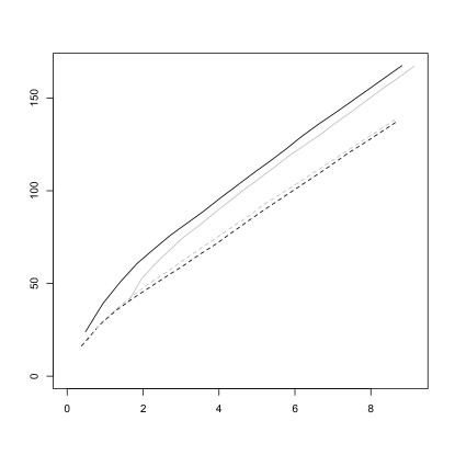
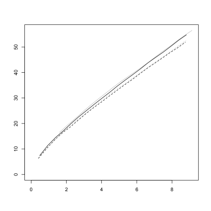
$|A|=1$	$|A|=3$
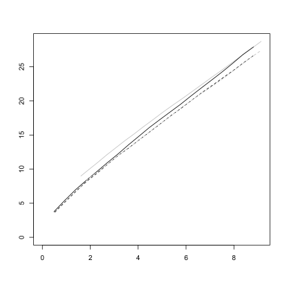
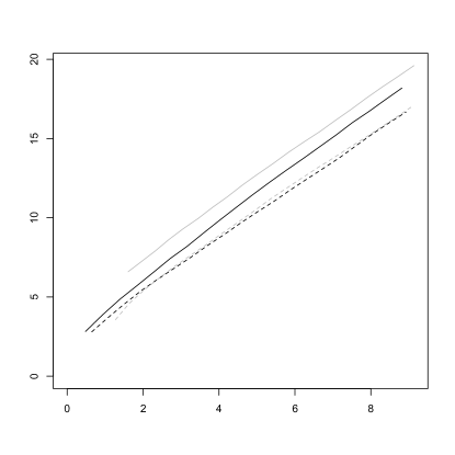
$|A|=6$	$|A|=9$

Figure 1: Expected sample size against the type-I error probability in log-scale for the G-SLRT (soft lines) and the M-SLRT (dark lines). That is, if $\mathcal{A}$ is the affected subset, we plot ${\sf E}^{\mathcal{A}}[T]$ (vertical axis) against $|\log{\sf P}_{0}(d=1)|$ (horizontal axis) for the following cases: $|\mathcal{A}|=1,3,6,9$. For both tests, solid lines refer to the case of no prior information ($\overline{\mathcal{P}}_{K}$), whereas dashed lines refer to the case that the size of the affected subset is known in advance ($\mathcal{P}_{|\mathcal{A}|}$).

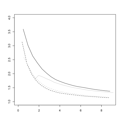
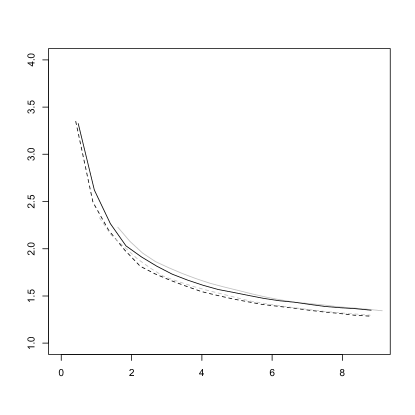
$|A|=1$	$|A|=3$
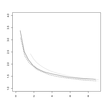
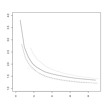
$|A|=6$	$|A|=9$

Figure 2: Normalized expected sample size against the type-I error probability in log-scale for the G-SLRT (soft lines) and the M-SLRT (dark lines). That is, if $\mathcal{A}$ is the affected subset, we plot $|\mathcal{A}|I_{1}{\sf E}^{\mathcal{A}}[T]/\,|\log{\sf P}_{0}(d=1)|$ (vertical axis) against $|\log{\sf P}_{0}(d=1)|$ (horizontal axis) for the following cases: $|\mathcal{A}|=1,3,6,9$. For both tests, solid lines refer to the case of no prior information ($\overline{\mathcal{P}}_{K}$), whereas dashed lines refer to the case that the size of the affected subset is known in advance ($\mathcal{P}_{|\mathcal{A}|}$).

VIII Conclusion and Remarks

We considered the problem of sequential detection of an unknown number of signals in multiple data streams and studied two families of sequential tests. The first, G-SLRT, is based on maximizing the likelihood ratios between the “signal and noise” and “noise only” hypotheses. The second, M-SLRT, is based on a mixture (weighted sum) of likelihood ratios. Based on the concept of $r$-complete convergence, we developed a general theory that allows for the study of asymptotic properties of the above sequential tests for very general non-i.i.d. models without assuming any particular structure for the observations apart from an asymptotic stability property of the local log-likelihood ratios. Specifically, under the assumption that the log-likelihood ratios in channels converge $r$-completely when suitably normalized, we were able to show that both tests asymptotically minimize moments of the sample size up to order $r$ as the probabilities of errors approach zero. Moreover, in the special case that the local log-likelihood ratios have independent (but not necessarily identically distributed) increments and converge only almost surely when suitably normalized, we showed that both tests asymptotically minimize all moments of the sample size.

These asymptotic optimality results were shown under the assumption of an arbitrary class of possibly affected subsets. They are thus valid for both structured and unstructured multistream hypothesis testing problems. Moreover, we illustrated this general sequential hypothesis testing theory using several meaningful examples including Markov and hidden Markov models, as well as a multichannel generalization of the famous invariant $t$-SPRT. Finally, when compared using a simulation study, the G-SLRT (M-SLRT) was found to perform better when a small (large) number of channels is affected and there is no prior information regarding the affected subset. On the other hand, the two procedures were found to perform similarly when the size of the affected subset is known in advance.

When the observations in channels are i.i.d., even if they differ across channels, we can obtain stronger and more refined results for the proposed procedures along the lines of our previous works [25, 26], such as near-optimality and higher order approximations. These results are based on nonlinear renewal theory and will be presented in the companion paper [19]. Moreover, it is also possible to generalize our asymptotic analysis by allowing the number of channels to approach infinity, which is also a topic of the companion paper [19].

References

• [1] F.-K. Chang, “Structural health monitoring: Promises and challenges,” in Proceedings of the 30th Annual Review of Progress in Quantitative NDE (QNDE), Green Bay, WI, USA.   American Institute of Physics, Jul. 2003.
• [2] C. Sonesson and D. Bock, “A review and discussion of prospective statistical surveillance in public health,” Journal of the Royal Statistical Society A, vol. 166, pp. 5–21, 2003.
• [3] K.-L. Tsui, S. W. Han, W. Jiang, and W. H. Woodall, “A review and comparison of likelihood based charting methods,” IIE Transactions, vol. 44, no. 9, pp. 724–743, Sep. 2012.
• [4] S. E. Fienberg and G. Shmueli, “Statistical issues and challenges associated with rapid detection of bio-terrorist attacks,” Statistics in Medicine, vol. 24, no. 4, pp. 513–529, Jul. 2005.
• [5] H. Rolka, H. Burkom, G. F. Cooper, M. Kulldorff, D. Madigan, and W. K. Wong, “Issues in applied statistics for public health bioterrorism surveillance using multiple data streams: research needs,” Statistics in Medicine, vol. 26, no. 8, pp. 1834–1856, 2007.
• [6] P. A. Bakut, I. A. Bolshakov, B. M. Gerasimov, A. A. Kuriksha, V. G. Repin, G. P. Tartakovsky, and V. V. Shirokov, Statistical Radar Theory.   Moscow, USSR: Sovetskoe Radio, 1963, vol. 1 (G. P. Tartakovsky, Editor), in Russian.
• [7] A. G. Tartakovsky and J. Brown, “Adaptive spatial-temporal filtering methods for clutter removal and target tracking,” IEEE Transactions on Aerospace and Electronic Systems, vol. 44, no. 4, pp. 1522–1537, Oct. 2008.
• [8] P. Szor, The Art of Computer Virus Research and Defense.   Upper Saddle River, NJ, USA: Addison-Wesley Professional, 2005.
• [9] A. G. Tartakovsky, “Rapid detection of attacks in computer networks by quickest changepoint detection methods,” in Data Analysis for Network Cyber-Security, N. Adams and N. Heard, Eds.   London, UK: Imperial College Press, 2014, pp. 33–70.
• [10] A. G. Tartakovsky, B. L. Rozovskii, R. B. Blaźek, and H. Kim, “Detection of intrusions in information systems by sequential change-point methods,” Statistical Methodology, vol. 3, no. 3, pp. 252–293, Jul. 2006.
• [11] ——, “A novel approach to detection of intrusions in computer networks via adaptive sequential and batch-sequential change-point detection methods,” IEEE Transactions on Signal Processing, vol. 54, no. 9, pp. 3372–3382, Sep. 2006.
• [12] D. Siegmund, “Change-points: From sequential detection to biology and back,” Sequential Analysis, vol. 32, no. 1, pp. 2–14, Jan. 2013.
• [13] A. G. Tartakovsky, “Discussion on “Change-points: From sequential detection to biology and back” by david siegmund,” Sequential Analysis, vol. 32, no. 1, pp. 36–42, Jan. 2013.
• [14] A. G. Tartakovsky, X. R. Li, and G. Yaralov, “Sequential detection of targets in multichannel systems,” IEEE Transactions on Information Theory, vol. 49, no. 2, pp. 425–445, Feb. 2003.
• [15] G. Fellouris and G. Sokolov, “Second-order asymptotic optimality in multichannel sequential detection,” IEEE Transactions on Information Theory, Submitted (arXiv:1410.3815).
• [16] Y. Mei, “Efficient scalable schemes for monitoring a large number of data streams,” Biometrika, vol. 97, no. 2, pp. 419–433, Apr. 2010.
• [17] Y. Xie and D. Siegmund, “Sequential multi-sensor change-point detection,” Annals of Statistics, vol. 41, no. 2, pp. 670–692, Mar. 2013.
• [18] A. G. Tartakovsky, I. V. Nikiforov, and M. Basseville, Sequential Analysis: Hypothesis Testing and Changepoint Detection, ser. Monographs on Statistics and Applied Probability.   Boca Raton, London, New York: Chapman & Hall/CRC Press, 2014.
• [19] G. Fellouris and A. G. Tartakovsky, “Multichannel sequential detection—Part II: i.i.d. data.” IEEE Transactions on Information Theory, Work in Progress.
• [20] P. L. Hsu and H. Robbins, “Complete convergence and the law of large numbers,” Proceedings of the National Academy of Sciences of the United States of America, vol. 33, no. 2, pp. 25–31, Feb. 1947.
• [21] L. E. Baum and M. Katz, “Convergence rates in the law of large numbers,” Transactions of the American Mathematical Society, vol. 120, no. 1, pp. 108–123, Oct. 1965.
• [22] A. V. Balakrishnan, Kalman Filtering Theory (Enlarged 2nd ed.), ser. Series in Communications and Control Systems.   Optimization Software, Inc., Publications Division, 1987.
• [23] M. Basseville and I. V. Nikiforov, Detection of Abrupt Changes – Theory and Application, ser. Information and System Sciences Series.   Englewood Cliffs, NJ, USA: Prentice-Hall, Inc, 1993, Online.
• [24] S. Pergamenchtchikov and A. G. Tartakovsky, “Asymptotically optimal pointwise and minimax quickest change-point detection for dependent data,” Statistical Inference for Stochastic Processes, Submitted in 2016.
• [25] G. Fellouris and A. G. Tartakovsky, “Nearly minimax one-sided mixture-based sequential tests,” Sequential Analysis, vol. 31, no. 3, pp. 297–325, 2012.
• [26] ——, “Almost optimal sequential tests of discrete composite hypotheses,” Statistica Sinica, vol. 23, no. 4, pp. 1717–1741, 2013.
• [27] A. Gut, Stopped Random Walks: Limit Theorems and Applications, ser. Series in Applied Probability.   New York, USA: Springer-Verlag, 1988, vol. 5.