Duality of a compact topological superconductor model and the Witten effect

Abstract

We consider a compact abelian Higgs model in 3+1 dimensions with a topological axion term and construct its dual theories for both bulk and boundary at strong coupling. The model may be viewed as describing a superconductor with magnetic monopoles, which can also be interpreted as a field theory of a topological Mott insulator. We show that this model is dual to a non-compact topological field theory of particles and vortices. It has exactly the same form of a model for superconducting cosmic strings with an axion term. We consider the duality of the boundary field theory at strong coupling and show that in this case $\theta$ is quantized as $-8\pi n/m$ where $n$ and $m$ are the quantum numbers associated to electric and magnetic charges. These topological states lack a non-interacting equivalent.

I Introduction

A plethora of topological states of matter have been identified and classified during the past decade Hasan-Kane-RMP ; Zhang-RMP-2011 ; Classif . These include material realizations such as strong topological insulators (STI). Interestingly, the microscopic electronic structure of these materials can be very different. However, some properties of an STI, set by topology, are universal. A celebrated example is the bulk-boundary correspondence guaranteeing the presence of surface states that are protected by the bulk topology. Another incarnation of this universality arises in the field-theoretical description of the electromagnetic response of STIs: it is governed by the canonical Maxwell Lagrangian supplemented by a topological term - the axion or $\theta$-term, $\sim\theta~{}{\bf E}\cdot{\bf B}$, which quantizes the electromagnetic response Qi-2008 .

Instead of an STI we consider a compact abelian Higgs model in 3+1 dimensions with a $\theta$-term Ryu-2012 ; Qi-Witten-Zhang ; Roy ; Nogueira-Sudbo-Eremin , which may be interpreted as an effective field theory for a topological Mott insulator and show that it is dual to an axionic superconductor model Ryu-2012 ; Qi-Witten-Zhang ; Roy ; Nogueira-Sudbo-Eremin where both particle and vortex degrees of freedom appear in the Lagrangian. The Lagrangian of the dual theory is similar to the one of a model for superconducting vortex strings Witten-SC-strings , except that it also features a $\theta$-term, which causes a topologically induced charge coupling for the vortex lines. Such an interacting field theory can be physically understood in terms of an experimental setup consisting of a superconducting slab sandwiched between two semi-infinite STIs (see Fig. 1). The $\theta$-term of the STI couples to the electrodynamics of vortex lines in the superconductor. This can be shown to lead to a charge fractionalization mechanism at the interfaces similar to the Witten effect, although no magnetic monopoles are present in this setting (see Section II). Thus, the Witten effect with charge fractionalization due to magnetic monopoles in the compact abelian Higgs model with an axion term maps via duality into a Witten effect associated to vortex lines.

It is well-known that without the topological axion term the compact Maxwell theory in 3+1 dimensions exhibits a confinement-deconfinement transition Guth . This transition can be understood by exploiting the duality of the compact Maxwell theory to the non-compact abelian Higgs model Peskin . In the dual Higgs model vortex lines correspond to worldlines of magnetic monopoles in the original model. Hence, the phase transition in the dual Higgs model corresponds to the confinement-deconfinement transition in the original compact U(1) Maxwell electrodynamics. The situation in 3+1 dimensions is quite different from the one in 2+1 dimensions where test charges are permanently confined Polyakov , with the Wilson loop satisfying the area law. Indeed, it is well known that compact Maxwell theory in 2+1 dimensions is dual to a Coulomb gas of magnetic monopoles (actually in this case it is more technically correct to speak of instantons). The sine-Gordon Lagrangian yields an exact field theory representation of a Coulomb gas in any dimensions Froehlich-Spencer-1981 . In 2+1 dimensions the sine-Gordon theory is always gapped, so no phase transition occurs in this case Polyakov ; Goepfer-Mack .

The duality transformation can also be carried out for the case of a compact abelian Higgs model. The exact result has been obtained for a model defined on a $d$-dimensional lattice long time ago Einhorn . Generally, when Higgs fields are included, the dual model is given by a vector or tensor Coulomb gas, depending on the dimensionality. In this paper we will find it useful to consider besides the complete duality transformation leading to a Coulomb gas, also a partial duality transformation, where the Higgs field is still present, while the magnetic monopole degrees of freedom are mapped on a dual Higgs sector representing the ensemble of world lines of magnetic monopoles as vortex lines. The resulting model in 3+1 dimensions corresponds to one of superconducting vortex strings mentioned above. If the original Higgs and gauge fields are also integrated out, the field theory corresponding to the duality discussed on the lattice by Cardy Cardy-theta and Cardy and Rabinovici Cardy-Rabinovici is obtained.

There is a question as to what happens with the duality at the boundary, which is important for topological states of matter. The compact Maxwell theory in 3+1 dimensions has a (2+1)-dimensional boundary. Thus, naively, we may think that the boundary theory is just compact Maxwell electrodynamics in 2+1 dimension. In such a case, the theory at the boundary will not exhibit a phase transition while the theory in the bulk will. However, this naive expectation clearly fails for the corresponding dual theory, since using the same logic we would expect that the dual model at the boundary is just the dimensionally reduced theory, i.e., the abelian Higgs model in 2+1 dimensions. This is obviously not the case, since the dual of compact Maxwell theory in 2+1 dimension is a sine-Gordon theory. Thus, the correct prescription to find the boundary dual theory is to dualize the dimensionally reduced model at the boundary. For the case of the axionic Higgs model we consider, the $\theta$-term generates a Chern-Simons term at the boundary. We will show that in this case $\theta$ becomes fractionally quantized in the infinitely coupled regime.

The plan of the paper is as follows. In Section II we discuss the Witten effect and derive a variant of it that also works with vortex lines. This result will serve to relate our duality to a physical problem of topological insulators coupled to type II superconductors Josephson-Witten . In Section III, we introduce the compact axionic abelian Higgs model and show that it is equivalent to a non-compact model for superconducting vortex strings, thus establishing an exact mapping between a Higgs model containing monopoles and a model containing vortices and two Higgs fields. In Section IV we discuss the duality transformation building on the results obtained in Section III. Section V discusses the boundary dual theory at strong coupling in the lattice. In Section VI we briefly comment on possible generalizations in the framework of quantum critical phenomena associated to the nonlinear $\sigma$ model. Section VII concludes the paper and in Appendix A we give further details on the calculations presented in the main text.

II Witten effect in electrodynamics

II.1 Electromagnetic variant of the Witten effect with monopoles and vortex lines

The Lagrangian for electrodynamics with an axion term is given by

$${\cal L}=\frac{1}{8\pi}({\bf E}^{2}-{\bf B}^{2})+\frac{e^{2}\theta}{4\pi^{2}}{\bf E}\cdot{\bf B}-\rho\phi-{\bf j}\cdot{\bf A}.$$ (1)

The standard Maxwell equations are modified by the presence of the $\theta$ term. The new relations are easily obtained by computing the electric displacement vector ${\bf D}$ and the magnetizing field ${\bf H}$ via

$${\bf D}=\frac{\partial{\cal L}}{\partial{\bf E}},~{}~{}~{}~{}~{}~{}~{}{\bf H}=-\frac{\partial{\cal L}}{\partial{\bf B}},$$ (2)

and inserting these results in the standard Maxwell equations. The important equation for the Witten effect is the Gauss law,

$${\mbox{\boldmath$\nabla$}}\cdot{\bf E}=4\pi\rho-\frac{e^{2}}{\pi}{\mbox{\boldmath$\nabla$}}\cdot(\theta{\bf B}).$$ (3)

Thus, unless magnetic monopoles are present, the Gauss law does not change if $\theta$ is uniform. Since ${\mbox{\boldmath$\nabla$}}\cdot{\bf B}=\rho_{m}$, where $\rho_{m}$ is the magnetic monopole density, the integral form of the Gauss law reads

$$Q=q-\frac{e^{2}\theta}{4\pi^{2}}q_{m}-\frac{e^{2}}{4\pi^{2}}\int_{V}d^{3}r{\mbox{\boldmath$\nabla$}}\theta\cdot{\bf B}.$$ (4)

Here, $q_{m}$ is the magnetic charge, which fulfills the Dirac condition, $qq_{m}=2\pi$. If $\theta$ is uniform and $q=ne$ (with integer $n$), Eq. (4) yields the charge fractionalization by monopoles of the Witten effect Witten-effect ,

$$Q=e\left(n-\frac{\theta}{2\pi}\right).$$ (5)

In a condensed matter system we generally do not have intrinsic magnetic monopoles, but surface states provide yet another form of the Witten effect, due to the last term of Eq. (4). Indeed, although in STIs $\theta$ is uniform, the presence of a surface leads to a nonzero value for the integral in Eq. (4). Thus, if $\theta$ has a uniform value for surfaces at $z=0$ and $z=L$, and ${\bf B}=B(r)\hat{\bf z}$ depends only on the radial coordinate $r$, we will obtain after setting $q_{m}=0$,

$$Q = q-\frac{e^{2}}{4\pi^{2}}\int_{0}^{L}dz\frac{d\theta}{dz}\int d^{2}rB(r)$$ (6)

$$= q-\frac{e^{2}}{4\pi^{2}}[\theta(L)-\theta(0)]\Phi_{B}.$$

The above constitutes a variant of the Witten effect when the magnetic flux $\Phi_{B}$ is nonzero. Fig. 1 illustrates a physical situation where Eq. (6) is realized, with a type II superconductor is sandwiched between two STIs (see also Ref. Josephson-Witten for another, closely related, example). If an external magnetic field is applied perpendicular to the interfaces, a flux line vortex lattice will arise and the magnetic flux will be nonzero. For STIs we generally have $\theta(L)=-\theta(0)=\theta$, with $\theta=\pi$ for time-reversal (TR) invariant systems. Using $q=n(2e)$ (with $(2e)$ the Cooper pair charge) and considering a total flux $\Phi_{B}$ due to $N_{v}$ straight vortex lines, we obtain the total charge,

$$Q=e\left(2n-\frac{\theta N_{v}}{2\pi}\right).$$ (7)

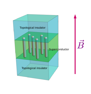
Figure 1: (Color online) Schematic view of a type II superconductor sandwiched between two STIs in presence of a magnetic field $\vec{B}$. Due to the topological magnetoelectric effect, the vortex lines, represented by straight flux tubes, acquire an electric polarization.

II.2 The Hall conductivity and the Witten effect

If there are no magnetic monopoles, we can derive the Hall conductivity from the current density obtained from Eq. (1)., by assuming that there is an interface separating a topologically trivial insulator ($\theta=0$) from a topologically nontrivial one ($\theta\neq 0$). We then find a dissipationless Hall current Josephson-Witten given by,

$${\bf j}_{H}=-\frac{e^{2}}{4\pi^{2}}({\mbox{\boldmath$\nabla$}}\theta\times{\bf E}).$$ (8)

If we consider an electric field applied at the surface $z=0$, e.g., ${\bf E}=E\hat{\bf x}$, we obtain the transverse surface current

$$i_{y}=-\frac{e^{2}E}{4\pi^{2}}\int_{0}^{\infty}dz\frac{d\theta}{dz}=\sigma_{xy}E,$$ (9)

where the Hall conductivity Sitte2012 ,

$$\sigma_{xy}=\frac{e^{2}}{2\pi}\left(n-\frac{\theta}{2\pi}\right).$$ (10)

We note the similarity between the expression for the charge, Eq. (5) and the one for the Hall conductivity, Eq. (10). In the following, we will show that for the case of topological superconductors this is not a mere accident (note, however, that a superconductor has elementary charge $2e$ rather than $e$).

This can already be seen by considering the very simple problem of a charged particle of mass $M$ constrained to move on a ring of radius $r$ and in the presence of a magnetic flux, $\Phi$. In this exactly solvable example it is easy to see that the current is given by,

$$j_{n}=-e\frac{dE_{n}}{d\Phi}=\frac{e^{3}}{2\pi Mr^{2}}\left(n-\frac{e\Phi}{2\pi}\right),$$ (11)

where

$$E_{n}(\Phi)=\frac{1}{2Mr^{2}}\left(n-\frac{e\Phi}{2\pi}\right)^{2},~{}~{}~{}~{}~{}~{}~{}~{}n\in\mathbf{Z},$$ (12)

are the exact energy eigenvalues.

III Compact Abelian Higgs model with axion term

Since the Witten effect in axion electrodynamics arises either in the presence magnetic monopoles or vortices, a general Abelian Higgs model accounting for both topological defects is given by the Lagrangian written in imaginary time,

$$\!\!\!\!{\cal L}=\frac{1}{4}{\cal F}_{\mu\nu}^{2}+\frac{ie^{2}\theta}{16\pi^{2}}{\cal F}_{\mu\nu}\tilde{\cal F}_{\mu\nu}+\frac{\rho^{2}}{2}(\partial_{\mu}\varphi+2eA_{\mu})^{2}+\frac{1}{2\rho_{V}^{2}}m_{\mu}^{2}.$$ (13)

Here, the field strength and its dual are given by Cardy ,

$${\cal F}_{\mu\nu}=F_{\mu\nu}+\frac{\pi}{e}\tilde{M}_{\mu\nu},~{}~{}~{}~{}~{}~{}$$ (14)

and

$$\tilde{\cal F}_{\mu\nu}=\tilde{F}_{\mu\nu}+\frac{\pi}{e}M_{\mu\nu}.$$ (15)

with $F_{\mu\nu}=\partial_{\mu}A_{\nu}-\partial_{\nu}A_{\mu}$ and $\tilde{F}_{\mu\nu}=(1/2)\epsilon_{\mu\nu\lambda\rho}F_{\mu\nu}$. We also have that $M_{\mu\nu}=\partial_{\mu}M_{\nu}-\partial_{\nu}M_{\mu}$ and $\tilde{M}_{\mu\nu}=(1/2)\epsilon_{\mu\nu\lambda\rho}M_{\mu\nu}$ where

$$M_{\mu}(x)=\int d^{4}x^{\prime}G(x-x^{\prime})m_{\mu}(x^{\prime}),$$ (16)

with the Coulomb Green function $G(x)=1/(4\pi^{2}x^{2})$. The field $m_{\mu}(x)$ is conserved and has the meaning of a magnetic monopole current. Thus, $M_{\mu}(x)$ is a monopole gauge field. We automatically have that $\partial_{\mu}M_{\mu}=0$ in view of the conservation of the monopole current; it follows that $\partial_{\mu}\tilde{\cal F}_{\mu\nu}=(\pi/e)m_{\nu}$, as expected. We will later see that the parameter $\rho_{V}$ emulates vortex stiffness. The way in which it appears in Eq. (13), $\rho_{V}^{-1}$ represents the chemical potential of monopoles. As discussed in Ref. Cardy , the field strength ${\cal F}_{\mu\nu}$ is a four-dimensional generalization of the superfluid velocity of two-dimensional superfluids NelKost . The magnetic monopole contribution accounts for the compactness of the local $U(1)$ gauge group in the same way that point vortices in two-dimensional superfluids account for the periodicity of the phase of the superfluid wavefunction Cardy . This procedure allows one to incorporate the periodicity of lattice fields in a continuum field theory approach where the fields become multivalued KleinertMultival .

In the absence of magnetic monopoles ($m_{\mu}=0$), Eq. (13) describes a three-dimensional superconductor with a $\theta$-term, which can be realized via a heterostructure like the one shown in Fig. 1. For $\theta=0$ and in the presence of monopoles, the phase structure of Eq. (13) has been discussed in the past using a lattice gauge theory formulation FS , where it has been pointed out that the model with two units of charge features three phase rather than two. Indeed, for the case of one unit of charge the Higgs and confinement phases cannot be distinguished, differently of the case with two units of charge. The third phase in the problem is the Coulomb phase. There is a first-order phase transition between the Higgs and the confined phases Lattice-Higgs . For $\theta\neq 0$ a first-order transition between the Higgs and the confinemed phases is still expected, but there are several such transitions, which are labeled by the integer monopole charge $m$ Cardy-theta ; Cardy-Rabinovici .

Further insight into the theory (13) can be obtained by introducing an auxiliary field $h_{\mu}$ to rewrite it (see Appendix A) as,

$${\cal L}^{\prime} = \frac{1}{4}(F_{\mu\nu}^{2}+f_{\mu\nu}^{2})+i\frac{e^{2}\theta}{16\pi^{2}}F_{\mu\nu}\tilde{F}_{\mu\nu}+im_{\mu}\left(\frac{\pi}{e}h_{\mu}+\frac{e\theta}{4\pi}A_{\mu}\right)$$ (17)

$$+ \frac{\rho^{2}}{2}(\partial_{\mu}\varphi+2eA_{\mu})^{2}+\frac{1}{2\rho_{V}^{2}}m_{\mu}^{2},$$

where $f_{\mu\nu}=\partial_{\mu}h_{\nu}-\partial_{\nu}h_{\mu}$. Physically, the gauge field $h_{\mu}$ accounts for the magnetic flux inside the vortex lines, akin to the London theory. Now, in order to integrate out the monopole gauge field subject to the constraint $\partial_{\mu}m_{\mu}=0$, we introduce a Lagrange multiplier $\varphi_{V}$ enforcing the constraint and perform the Gaussian integration over $m_{\mu}$ to obtain,

$${\cal L} = \frac{1}{4}(F_{\mu\nu}^{2}+f_{\mu\nu}^{2})+i\frac{e^{2}\theta}{16\pi^{2}}F_{\mu\nu}\tilde{F}_{\mu\nu}$$ (18)

$$+ \frac{\rho^{2}}{2}(\partial_{\mu}\varphi+2eA_{\mu})^{2}+\frac{\rho_{V}^{2}}{2}\left(\partial_{\mu}\varphi_{V}+\frac{\pi}{e}h_{\mu}+\frac{e\theta}{4\pi}A_{\mu}\right)^{2}.$$

The above Lagrangian indicates that $\varphi_{V}$ physically represents the phase of a vortex disorder field and that $\rho_{V}$ can be indeed be interpreted as a vortex stiffness. Due to the magnetoelectric (axionic) coupling, the vortex current couples directly to the vector potential with charge $e\theta/(4\pi)$.

Despite similarities with the Ginzburg-Landau theory of three-dimensional topological superconductors discussed in Ref. Qi-Witten-Zhang , Eq. (18) has a very different physical content. The theory of Ref. Qi-Witten-Zhang features two superconducting order parameters coupled to the vector potential with charge $2e$, and $\theta$ is the phase difference between the phases of each order parameter. Furthermore, the gauge field $h_{\mu}$ is absent.

The Lagrangian (18) for $\theta=0$ is a model for superconducting cosmic strings introduced by Witten quite some time ago Witten-SC-strings . Note that the presence of the $\theta$-term leads to a fractionalization of the vortex string charge. Indeed, the vortex string charge is given by,

$$Q_{V} = S\int_{L}ds\left[\vphantom{\frac{e\theta}{4\pi}}2e\rho^{2}(\partial_{t}\varphi+2eA_{0})\right.$$ (19)

$$+ \left.\frac{e\theta}{4\pi}\rho_{V}^{2}\left(\partial_{t}\varphi_{V}+\frac{\pi}{e}h_{0}+\frac{e\theta}{4\pi}A_{0}\right)\right],$$

where $S$ corresponds to a cross-sectional area of the string and the integral is along a path $L$ defined by the vortex line, which can also form closed loops in general. For $\theta=0$ the above equation reduces to the standard formula for the vortex charge.

IV Electromagnetic duality

IV.1 Dual model

In the absence of matter fields (i.e., $\rho=0$), the Lagrangian (13) reduces to a compact Maxwell theory with an axion term. Note that for $\theta=0$ the two Higgs sectors in Eq. (18) decouple. The corresponding Higgs electrodynamics of vortices that is obtained in this way corresponds precisely to the model dual to the compact Maxwell theory in 3+1 dimensions Peskin . For $\theta\neq 0$, the gauge field $A_{\mu}$ remains coupled to the vortex Higgs model when $\rho=0$. The compact Maxwell theory with an axion term has the same form as the Lagrangian for the electrodynamics of a topological insulator Qi-2008 , except that the latter case does not include magnetic monopoles. We may interpret the compact version of the axion electrodynamics of topological insulators as a model for topological interacting systems, like topological Mott insulators Senthil_Science-2014 .

Up to the surface term, the Lagrangian (18) has an electromagnetic self-duality made transparent by a shift $h_{\mu}\to h_{\mu}-\frac{e^{2}\theta}{4\pi^{2}}A_{\mu}$, followed by the rescalings, $h_{\mu}\to 2eh_{\mu}$, $A_{\mu}\to(\pi/e)A_{\mu}$. Following these, the Lagrangian reads

$${\cal L} = \frac{1}{4}\left[\begin{array}[]{cc}F_{\mu\nu}&f_{\mu\nu}\end{array}\right]\left[\begin{array}[]{cc}\frac{\pi^{2}}{e^{2}}+\frac{e^{2}\theta^{2}}{16\pi^{2}}&-\frac{e^{2}\theta}{2\pi}\\ \vskip 6.0pt plus 2.0pt minus 2.0pt\cr-\frac{e^{2}\theta}{2\pi}&4e^{2}\end{array}\right]\left[\begin{array}[]{c}F_{\mu\nu}\\ \vskip 6.0pt plus 2.0pt minus 2.0pt\cr f_{\mu\nu}\end{array}\right]+i\frac{\theta}{16}F_{\mu\nu}\tilde{F}_{\mu\nu}$$ (25)

$$+ \frac{\rho^{2}}{2}(\partial_{\mu}\varphi+2\pi A_{\mu})^{2}+\frac{\rho_{V}^{2}}{2}(\partial_{\mu}\varphi_{V}+2\pi h_{\mu})^{2}.$$ (26)

From the above representation a duality first discussed in Ref. Cardy-theta in the context of a $U(1)$ lattice gauge theory is obtained. It is given by the transformations,

$$e^{\prime}=\frac{1}{2}\sqrt{\frac{\pi^{2}}{e^{2}}+\frac{e^{2}\theta^{2}}{16\pi^{2}}},~{}~{}~{}~{}~{}~{}~{}\theta^{\prime}=-\frac{4\theta e^{2}}{\frac{\pi^{2}}{e^{2}}+\frac{e^{2}\theta^{2}}{16\pi^{2}}},$$ (27)

with the field transformations, $A_{\mu}\to h_{\mu},~{}h_{\mu}\to-A_{\mu},~{}\{\varphi\to\varphi_{V},~{}\rho\to\rho_{V}\},$ and $\{\varphi_{V}\to-\varphi,~{}\rho_{V}\to\rho\}$, such that the Lagrangian is invariant up to the surface ($\theta$-) term, meaning that the Lagrangian is self-dual in the bulk. From Eq. (25), we realize that Eq. (27) implies that the Dirac duality $e^{2}e^{\prime 2}=\pi^{2}/4$ of the $\theta=0$ case is replaced by a matrix relation $MM^{\prime}=(\pi^{2}/4)I$ when $\theta\neq 0$. Here, $M$ is the matrix appearing in Eq. (25), and $I$ is a $2\times 2$ identity matrix Note-1 . This electromagnetic duality emulates a symmetry, since broadly, dualities are unitary transformations that become symmetries at self-dual points Zohar-PRL-2010 . In the context of topological states, symmetry related aspects of duality have been recently studied in terms of interacting Dirac fermions Wang-Senthil ; Metlitski-Vishwanath ; Witten-2015 ; Metlitski-2015 ; Fradkin-2015 .

We can integrate out $\varphi$ in Eq. (17) by introducing a conserved charge current $j_{\mu}$ to obtain,

$${\cal L}^{\prime} = \frac{1}{4}(F_{\mu\nu}^{2}+f_{\mu\nu}^{2})+i\frac{e^{2}\theta}{16\pi^{2}}F_{\mu\nu}\tilde{F}_{\mu\nu}+i\frac{\pi}{e}m_{\mu}h_{\mu}$$ (28)

$$+ ie\left(2j_{\mu}+\frac{\theta}{4\pi}m_{\mu}\right)A_{\mu}+\frac{1}{2\rho^{2}}j_{\mu}^{2}+\frac{1}{2\rho_{V}^{2}}m_{\mu}^{2}.$$

Due to the $\theta$-term, the gauge field $A_{\mu}$ couples to both charge and monopole currents, implying that the physical current is

$$eJ_{\mu}=2ej_{\mu}+\frac{e\theta}{4\pi}m_{\mu}.$$ (29)

Thus, integrating $eJ_{0}$ over the volume yields,

$$Q=e\left(2n+m\frac{\theta}{4\pi}\right),$$ (30)

where $n,m\in\mathbb{Z}$, and we have assumed the normalizations,

$$\int d^{3}x~{}j_{0}(x)=n,~{}~{}~{}~{}~{}~{}\int d^{3}x~{}m_{0}(x)=m,$$ (31)

which shows that Eq. (30) is yet another incarnation of the Witten effect. From Eq. (30) we note the invariance $\theta\to\theta+8\pi$, $n\to n-m$ as a consequence of the periodicity of $\theta$ Cardy-theta . Setting $j_{\mu}=0$ and $m_{\mu}=0$ reduces to the situation of a non-interacting topological insulator Qi-2008 . We further distinguish here the following relevant special cases. When $j_{\mu}=0$ and $m_{\mu}\neq 0$, the theory describes an interacting topological insulator, since no charge is flowing and the gauge field is compact. If both $j_{\mu}$ and $m_{\mu}$ are nonzero, a polarized state of dipoles made of one electric and one magnetic charge, the so called dyon Schwinger-1969 , may form. If such polarized dyonic system is overall charge neutral, we obtain a diamagnetolectric rather than a dielectric type of insulator.

If we integrate out $A_{\mu}$ and $h_{\mu}$ in Eq. (28), we obtain the continuum version of the lattice dual model obtained by Cardy Cardy-theta and Cardy and Rabinovici Cardy-Rabinovici ,

$$\tilde{S} = \frac{1}{2}\left(\frac{\pi^{2}}{e^{2}}+\frac{e^{2}\theta^{2}}{16\pi^{2}}\right)\int d^{4}x\int d^{4}x^{\prime}G(x-x^{\prime})m_{\mu}(x)m_{\mu}(x^{\prime})$$ (32)

$$+ \frac{(2e)^{2}}{2}\int d^{4}x\int d^{4}x^{\prime}G(x-x^{\prime})j_{\mu}(x)j_{\mu}(x^{\prime})$$

$$+ \frac{e^{2}\theta}{2\pi}\int d^{4}x\int d^{4}x^{\prime}G(x-x^{\prime})j_{\mu}(x)m_{\mu}(x^{\prime})$$

$$+ \int d^{4}x\left(\frac{1}{2\rho^{2}}j_{\mu}^{2}+\frac{1}{2\rho_{V}^{2}}m_{\mu}^{2}\right),$$

apart from the local quadratic terms $j_{\mu}^{2}$ and $m_{\mu}^{2}$. The electromagnetic duality (27) holds once more, provided that the replacements $m_{\mu}\to j_{\mu}$ and $j_{\mu}\to-m_{\mu}$ are made.

Vortices and (superfluid) particles have large stiffnesses in the lattice formulation of Ref. Cardy-theta or, equivalently, no chemical potentials for charge and magnetic currents. However, such local quadratic terms should be generated by short-distance fluctuations.

Note that when $\rho\to 0$, corresponding to the regime of a compact Maxwell theory with an axion term, the currents $j_{\mu}$ are frozen to zero, and the dual action (32) becomes a vector Coulomb gas of magnetic monopole currents.

IV.2 Renormalization aspects

From the electromagnetic self-duality (27) we see that $e^{\prime 2}\theta^{\prime}=-e^{2}\theta$ and that,

$$e^{\prime}e=\frac{1}{2}\sqrt{\pi^{2}+\frac{e^{4}\theta^{2}}{16\pi^{2}}},$$ (33)

must be invariant by renormalization, i.e., $e^{\prime}_{r}e_{r}=e^{\prime}e$, where the subindex $r$ denotes renormalized counterparts. If $Z_{A}$ is the wavefunction renormalization for the field $A_{\mu}$, we obtain from the Ward identities the usual result, $e^{2}_{r}=Z_{A}e^{2}$ following from gauge invariance. Thus, if $Z_{h}$ denotes the wavefunction renormalization for the field $h_{\mu}$, duality invariance immediately implies that $Z_{A}Z_{h}=1$. Therefore, if we use the Ward identities once more, we obtain,

$$\theta_{r}=\sqrt{Z_{A}Z_{h}}\theta=\theta,$$ (34)

implying that $\theta$ does not renormalize. Thus, we have,

$$e^{2}_{r}\theta_{r}F_{r,\mu\nu}\tilde{F}_{r,\mu\nu}=e^{2}\theta F_{\mu\nu}\tilde{F}_{\mu\nu},$$ (35)

implying that the axion term is a renormalization invariant. This is consistent with the topological character of the axion term as a topological term. Indeed, since it does not depend on the metric, we expect it to be insensitive to scale transformations and therefore it must not change under renormalization.

V Boundary theory and duality at strong-coupling

Since $F_{\mu\nu}\tilde{F}_{\mu\nu}=2\epsilon_{\mu\nu\lambda\rho}\partial_{\mu}(A_{\nu}\partial_{\lambda}A_{\rho})$, the $\theta$-term yields a Chern-Simons (CS) term at the boundary. Thus, if we consider a system defined with a boundary at $z=0$, the actual physics of the problem is described by a dimensionally reduced system in the strong-coupling limit. To see this we first write,

$$\frac{1}{4}F_{\mu\nu}^{2}=\frac{1}{2}(\epsilon_{\mu\nu\lambda}\partial_{\nu}A_{\lambda})^{2}+\frac{1}{2}(\partial_{z}A_{\mu}-\partial_{\mu}A_{z})^{2},$$ (36)

where now it is understood that the Greek indices on the RHS of the above equation refer to three-dimensional spacetime, $x_{\parallel}=(\tau,x,y)$, with a similar expression holding for $f_{\mu\nu}$. Thus, upon integrating out both $A_{z}$ and $h_{z}$, we obtain that the action associated to the Lagrangian (28) can be written in the form,

$$S^{\prime} = \frac{1}{2}\int d^{4}x\left[(\epsilon_{\mu\nu\lambda}\partial_{\nu}A_{\lambda})^{2}+(\epsilon_{\mu\nu\lambda}\partial_{\nu}h_{\lambda})^{2}+(\partial_{z}A_{\mu})^{2}+(\partial_{z}h_{\mu})^{2}+ieJ_{\mu}A_{\mu}+i\frac{\pi}{e}m_{\mu}h_{\mu}+\frac{1}{2\rho^{2}}j_{\mu}^{2}+\frac{1}{2\rho_{V}^{2}}m_{\mu}^{2}\right]$$ (37)

$$+ i\frac{e^{2}\theta}{8\pi^{2}}\int d^{3}x_{\parallel}\epsilon_{\mu\nu\lambda}A_{\mu}\partial_{\nu}A_{\lambda}+\frac{(2e)^{2}}{2}\int d^{3}x_{\parallel}\int d^{3}x_{\parallel}^{\prime}G_{3D}(x_{\parallel}-x_{\parallel}^{\prime})j_{z}(x_{\parallel})j_{z}(x_{\parallel}^{\prime})$$

$$+ \frac{1}{2}\left(\frac{\pi^{2}}{e^{2}}+\frac{e^{2}\theta^{2}}{16\pi^{2}}\right)\int d^{3}x_{\parallel}\int d^{3}x_{\parallel}^{\prime}G_{3D}(x_{\parallel}-x_{\parallel}^{\prime})m_{z}(x_{\parallel})m_{z}(x_{\parallel}^{\prime})+\frac{e^{2}\theta}{2\pi}\int d^{3}x_{\parallel}\int d^{3}x_{\parallel}^{\prime}G_{3D}(x_{\parallel}-x_{\parallel}^{\prime})j_{z}(x_{\parallel})m_{z}(x_{\parallel}^{\prime})$$

where $G_{3D}(x_{\parallel}-x_{\parallel}^{\prime})=1/(4\pi|x_{\parallel}-x_{\parallel}^{\prime}|)$ and,

$$j_{z}(x_{\parallel})=\int_{-\infty}^{\infty}dzj_{z}(x_{\parallel},z),~{}~{}~{}~{}~{}~{}~{}~{}~{}~{}m_{z}(x_{\parallel})=\int_{-\infty}^{\infty}dzm_{z}(x_{\parallel},z),$$ (38)

and we have used that $\theta(z)=\theta$ for $z\geq 0$, vanishing otherwise. The second and third lines of Eq. (37) contain only surface modes, while the bulk still contributes in the first line.

An interesting limiting case where the boundary theory decouples from the bulk is obtained by letting $e^{2}\to\infty$. By rescaling $A_{\mu}\to e^{-1}A_{\mu}$ and $h_{\mu}\to e^{-1}h_{\mu}$ in Eq. (28), the action for $e^{2}\to\infty$ becomes,

$$S_{\infty}=i\frac{\theta}{8\pi^{2}}\int d^{3}x_{\parallel}\epsilon_{\mu\nu\lambda}A_{\mu}\partial_{\nu}A_{\lambda}$$ (39)

$$+ \int d^{4}x\left[i\left(2j_{\mu}+\frac{\theta}{4\pi}m_{\mu}\right)A_{\mu}+\frac{1}{2\rho^{2}}j_{\mu}^{2}+\frac{1}{2\rho_{V}^{2}}m_{\mu}^{2}\right].$$

Because there is no Maxwell term in $S_{\infty}$, we have that $J_{\mu}=0$ in the bulk and the currents exist only on the surface, i.e., we have an insulating bulk. From Eq. (37) we also see that both $j_{z}$ and $m_{z}$ are constrained to vanish in the limit $e^{2}\to\infty$. Since $J_{\mu}$ vanishes in the bulk, Eq. (30) implies that $\theta/(8\pi)=-n/m$, $m\neq 0$. This result is consistent with Cardy’s discussion Cardy-theta of the phase structure of the lattice model, although the boundary theory has not been considered in Ref. Cardy-theta . There the critical point is attained at values $\theta/(2\pi)=-n/m$ (note the factor $2\pi$ instead of $8\pi$, which arises in our case because the charge of our bosons is $2e$), when the bare coupling becomes infinitely large.

Note that locking $\theta$ to $-8\pi n/m$ in the strong-coupling regime implies that $\theta$ cannot be smoothly connected to zero, corresponding to a situation similar to the one encountered recently Nogueira-Sudbo-Eremin in the renormalization group analysis of a three-dimensional topological superconductor of the type studied in Ref. Qi-Witten-Zhang . In the following we will elaborate further on this regime by means of the duality transformation.

A subtle aspect of the boundary theory following from Eq. (39) is uncovered when performing the Gaussian integral over $A_{\mu}$. Integrating out $A_{\mu}$ at the boundary leads to the effective Lagrangian at strong coupling ($J_{\mu}\neq 0$ at the boundary),

$$\tilde{\cal L}_{\infty}=i\frac{2\pi^{2}}{\theta}\epsilon_{\mu\nu\lambda}J_{\mu}\frac{\partial_{\nu}}{\partial^{2}}J_{\lambda}+\frac{1}{2\rho^{2}}j_{\mu}^{2}+\frac{1}{2\rho_{V}^{2}}m_{\mu}^{2}.$$ (40)

Solving the current conservation constraints yields, $j_{\mu}=\epsilon_{\mu\nu\lambda}\partial_{\nu}a_{\lambda}$ and $m_{\mu}=\epsilon_{\mu\nu\lambda}\partial_{\nu}b_{\lambda}$. Therefore,

$$\tilde{\cal L}_{\infty} = \frac{1}{2\rho^{2}}(\epsilon_{\mu\nu\lambda}\partial_{\nu}a_{\lambda})^{2}+\frac{1}{2\rho_{V}^{2}}(\epsilon_{\mu\nu\lambda}\partial_{\nu}b_{\lambda})^{2}$$ (41)

$$+ i\frac{2\pi^{2}}{\theta}\epsilon_{\mu\nu\lambda}\left(2a_{\mu}+\frac{\theta}{4\pi}b_{\mu}\right)\partial_{\nu}\left(2a_{\lambda}+\frac{\theta}{4\pi}b_{\lambda}\right).$$

If we define a two component gauge field $(h_{I\mu})=(a_{\mu},b_{\mu})$, we can rewrite the above Lagrangian in the form,

$$\tilde{\cal L}_{\infty}=\frac{1}{2}\sum_{I}\frac{1}{\rho_{I}}(\epsilon_{\mu\nu\lambda}\partial_{\nu}h_{I\lambda})^{2}+i\pi\epsilon_{\mu\nu\lambda}\sum_{I,J}K_{IJ}h_{I\mu}\partial_{\nu}h_{J\lambda},$$ (42)

where $\rho_{1}=\rho$ and $\rho_{2}=\rho_{V}$, and $K_{IJ}$ are the elements of the matrix,

$$K=\left[\begin{array}[]{cc}-m/n&1\\ \vskip 6.0pt plus 2.0pt minus 2.0pt\cr 1&-n/m\end{array}\right],$$ (43)

The result of a matrix CS term is reminiscent from effective theories for the fractional quantum Hall state Wen-Zee . Actually, our system is rather an anyon superfluid, as $\det K=0$, implying the existence of a gapless mode. Note, however, that the entries of the matrix $K$ are not necessarily integers in this case.

The Lagrangian (41) describes a free theory leading us to conclude that the strongly coupled theory at the boundary is non-interacting. However, this is an example where standard continuum manipulations yield an incorrect result. The Lagrangian (41) is actually incomplete, as an analysis made in the lattice will now demonstrate. The difficulty lies on the fact that solving the current conservation constraint in the continuum formulation misses in some cases the periodic character of phase variables that underly the current conservation itself. There is, in fact, a discrete periodicity in the current that cannot always be properly captured with a field-theoretical analysis performed directly in the continuum.

The lattice boundary theory associated with the bulk action (39) is

$$S_{\infty}^{b} = \sum_{l}\left[i\frac{\theta}{8\pi^{2}}\epsilon_{\mu\nu\lambda}A_{l\mu}\Delta_{\nu}A_{l\lambda}+i\left(2j_{l\mu}+\frac{\theta}{4\pi}m_{l\mu}\right)A_{l\mu}\right.$$ (44)

$$+ \left.\frac{1}{2\rho^{2}}j_{l\mu}^{2}+\frac{1}{2\rho_{V}^{2}}m_{l\mu}^{2}\right],$$

where the lattice derivative is defined in a standard way as $\Delta_{\mu}f_{l}=f_{l+1}-f_{l}$ (with unit lattice spacing). The currents $j_{l\mu}$ and $m_{l\mu}$ are now integer valued lattice fields, making the normalization superfluous. Thus, the partition function

$$Z_{\infty}^{b}=\sum_{\{j_{l\mu}\}}\sum_{\{m_{l\mu}\}}\delta_{\Delta_{\mu}j_{l\mu},0}\delta_{\Delta_{\mu}m_{l\mu},0}\int_{-\infty}^{\infty}\left[\prod_{j}dA_{j\mu}\right]e^{-S_{\infty}^{b}},$$ (45)

with the current conservation constraints being enforced by Kronecker deltas. Using the integral representation of the Kronecker deltas,

$$\delta_{\Delta_{\mu}n_{l\mu},0}=\int_{0}^{2\pi}\frac{d\varphi_{l}}{2\pi}e^{i\varphi_{l}\Delta_{\mu}n_{l\mu}},$$ (46)

$$\delta_{\Delta_{\mu}s_{l\mu},0}=\int_{0}^{2\pi}\frac{d\varphi_{Vl}}{2\pi}e^{i\varphi_{Vl}\Delta_{\mu}s_{l\mu}},$$ (47)

in Eq. (45), and applying once more the Poisson formula Note-3 ,

$$S_{\infty}^{b} = \sum_{l}\left[i\frac{\theta}{8\pi^{2}}\epsilon_{\mu\nu\lambda}A_{l\mu}\Delta_{\nu}A_{l\lambda}+\frac{\rho^{2}}{2}(\Delta_{\mu}\varphi_{l}-2\pi p_{l\mu}-2A_{l\mu})^{2}\right.$$ (48)

$$+ \left.\frac{\rho_{V}^{2}}{2}\left(\Delta_{\mu}\varphi_{Vl}-2\pi q_{l\mu}-\frac{\theta}{4\pi}A_{l\mu}\right)^{2}\right],$$

with another set of integer fields, $p_{l\mu}$ and $q_{l\mu}$.

Integrating over $A_{l\mu}$ yields a lattice version of Eq. (40) where the currents are integer fields. Solving the current conservation constraints yields integer-valued gauge fields, $j_{l\mu}=\epsilon_{\mu\nu\lambda}\Delta_{\nu}N_{l\lambda}$ and $m_{l\mu}=\epsilon_{\mu\nu\lambda}\Delta_{\nu}M_{l\lambda}$. This point is the key to understand why Eq. (41) is not quite correct. The corresponding lattice action has the same form as Eq. (41), but with integer-valued gauge fields. Introducing real-valued lattice gauge fields via the Poisson formula Note-2 , we obtain

$$\tilde{S}_{\infty}^{b} = \sum_{l}\left[\frac{1}{2\rho^{2}}(\epsilon_{\mu\nu\lambda}\Delta_{\nu}a_{l\lambda})^{2}+\frac{1}{2\rho_{V}^{2}}(\epsilon_{\mu\nu\lambda}\Delta_{\nu}b_{l\lambda})^{2}\right.$$ (49)

$$+ i\frac{2\pi^{2}}{\theta}\epsilon_{\mu\nu\lambda}\left(2a_{l\mu}+\frac{\theta}{4\pi}b_{l\mu}\right)\Delta_{\nu}\left(2a_{l\lambda}+\frac{\theta}{4\pi}b_{l\lambda}\right)$$

$$- \left.2\pi in_{l\mu}a_{l\mu}-2\pi is_{l\mu}b_{l\mu}\right],$$

where $n_{l\mu}$ and $s_{l\mu}$ are integer fields representing conserved currents, which in this case is a consequence of gauge invariance. In contrast to Eq. (41), due to the coupling of the gauge fields to the currents, Eq. (49) does not yield a free quadratic theory.

The action $\tilde{S}_{\infty}^{b}$ corresponds to the boundary dual of the action ${S}_{\infty}^{b}$. Besides realizing that the theory given by Eq. (40) is actually not free, the dual transformation above shows that $\rho$ and $\rho_{V}$ of the action ${S}_{\infty}^{b}$ become the dielectric constants (or gauge couplings) in the dual action $\tilde{S}_{\infty}^{b}$. While ${S}_{\infty}^{b}$ is strongly coupled, $\tilde{S}_{\infty}^{b}$ is not. This allows us to find a regime where the boundary theory becomes self-dual. The self-dual regime is expediently explored using the actions of Eqs. (44,49). In Eq. (44), $m_{l\mu}$ vanishes when $\rho_{V}\to 0$. Similarly, in Eq. (49), $b_{l\mu}$ can be gauged away in this limit. Thus, by assuming the limit $\rho_{V}\to 0$ and rescaling $A_{l\mu}\to\pi A_{l\mu}$, we obtain the self-duality of the actions (44) and (49) at $\rho\to\infty$, provided $\theta/(8\pi)=\pm 1$, in which case the actions become precisely equivalent.

VI Possible generalizations

It is in principle possible to connect the compact Maxwell theory discussed in this paper to quantum spin models exhibiting an emergent $U(1)$ symmetry, like for example, those models described by the theory of deconfined quantum critical points Senthil-2004 . In order to put in perspective the types of bosonic topological states we are looking for in terms of spins models, we start by recalling some properties of deconfined critical points in 2+1 dimensions that are useful in this paper. We first consider a version of the Faddeev-Skyrme model FS-model ; Babaev as discussed similarly in Ref. Nogueira-Sudbo-2012 ,

$${\cal L}=\frac{1}{2g}(\partial_{\mu}{\bf n})^{2}+\frac{1}{2e^{2}}[\epsilon_{\mu\nu\lambda}\partial_{\nu}c_{\lambda}+\epsilon_{\mu\nu\lambda}{\bf n}\cdot(\partial_{\nu}{\bf n}\times\partial_{\lambda}{\bf n})]^{2},$$ (50)

where ${\bf n}^{2}=1$ and $c_{\mu}$ is a non-compact $U(1)$ gauge field. The strongly coupled regime $g\to\infty$ describes a nontrivial paramagnetic phase where the Lagrangian (50) becomes a compact Maxwell theory. This can be shown by using ’t Hooft’s construction tHooft-1974 of an Abelian gauge field from a non-Abelian one. Indeed, we can write $F_{\mu\nu}={\bf n}\cdot{\bf F}_{\mu\nu}=\partial_{\mu}c_{\nu}-\partial_{\nu}c_{\mu}+{\bf n}\cdot(\partial_{\mu}{\bf n}\times\partial_{\nu}{\bf n})$, where ${\bf F}_{\mu\nu}=\partial_{\mu}{\bf J}_{\nu}-\partial_{\nu}{\bf J}_{\mu}-{\bf J}_{\mu}\times{\bf J}_{\nu}$ is a non-Abelian field strength associated with the $O(3)$ gauge field, ${\bf J}_{\mu}={\bf n}c_{\mu}+{\bf n}\times\partial_{\mu}{\bf n}$. Since,

$$Q=\frac{1}{8\pi}\oint_{S}dS_{\mu}\epsilon_{\mu\nu\lambda}{\bf n}\cdot(\partial_{\nu}{\bf n}\times\partial_{\lambda}{\bf n}),$$ (51)

where $Q\in\mathbb{Z}$, the $g\to\infty$ limit of the theory dualizes to a sine-Gordon theory with $\pi/2$ periodicity, rather than the usual $2\pi$ one of Polyakov’s compact Maxwell theory in 2+1 dimensions Polyakov . Physically the $\pi/2$ periodicity represents the $\pi/2$ rotations mapping a VBS state into another one Senthil-2004 . Since the sine-Gordon model in 2+1 dimensions is always gapped, there is no phase transition occurring in the system. This gap leads to a finite string tension between spinons and anti-spinons in the original model, which impedes a deconfinement to occur. Since $[\epsilon_{\mu\nu\lambda}{\bf n}\cdot(\partial_{\nu}{\bf n}\times\partial_{\lambda}{\bf n})]^{2}=(\partial_{\mu}{\bf n}\times\partial_{\nu}{\bf n})^{2}$, and ${\bf n}$ is the direction of the spin, a lattice model associated to the compact Maxwell term would automatically include four-spin interactions between singlet bonds, similarly to the so called $J-Q$ model Sandvik_2007 . The limit $g\to\infty$ corresponds to the case where the four-spin singlet bond interaction dominates the physics.

A topologically nontrivial theory in 2+1 dimensions can be obtained by taking ’t Hooft’s construction one step further to add into the Lagrangian (50) the (non-abelian) CS term,

$${\cal L}_{\rm CS} = i\frac{\theta}{16\pi^{2}}\epsilon_{\mu\nu\lambda}\left[{\bf J}_{\mu}\cdot\partial_{\nu}{\bf J}_{\lambda}+\frac{1}{3}{\bf J}_{\mu}\cdot({\bf J}_{\nu}\times{\bf J}_{\lambda})\right]$$ (52)

$$= i\frac{\theta}{16\pi^{2}}\left[\epsilon_{\mu\nu\lambda}c_{\mu}\partial_{\nu}c_{\lambda}-\frac{2}{3}c_{\mu}\epsilon_{\mu\nu\lambda}{\bf n}\cdot(\partial_{\nu}{\bf n}\times\partial_{\lambda}{\bf n})\right].$$

One way to realize the above CS contribution in models of quantum criticality in 2+1 dimensions is to assume a physical situation where the quantum phase transition occurs on the surface of a (3+1)-dimensional system. In this case, the CS term arises from a so called $\theta$-term in the action of a (3+1)-dimensional theory, which has the well-known form,

$${\cal S}_{\theta}=i\frac{\theta}{32\pi^{2}}\int d^{4}x\epsilon_{\mu\nu\lambda\rho}{\bf F}_{\mu\nu}\cdot{\bf F}_{\lambda\rho}=i\frac{\theta}{32\pi^{2}}\int d^{4}x\partial_{\mu}K_{\mu},$$ (53)

where $K_{\mu}=2\epsilon_{\mu\nu\lambda\rho}[{\bf J}_{\nu}\cdot\partial_{\lambda}{\bf J}_{\rho}+(1/3){\bf J}_{\nu}\cdot({\bf J}_{\lambda}\times{\bf J}_{\rho})]$ is the CS current. Again, it is possible to define a compact abelian $\theta$-term from the non-abelian one. Within this point of view, a topological interacting state of matter in three dimensions mimics the electrodynamics of topological band insulators Qi-2008 , where a fluctuating field associated to topological defects leads to an emergent compact $U(1)$ symmetry.

VII Conclusions

We have constructed and exploited the dualities of a compact abelian Higgs model with a topological axion term and shown that it is equivalent to a topological, non-compact, abelian Higgs model having two Higgs and two gauge fields, akin to the model for superconducting vortex strings, but with a topological term. In other words, we have established the equivalence between a topological theory having bosonic particles coupled to monopoles in a gauge invariant way and a topological theory having bosonic particles and vortices. This equivalence allows us to better understand how the Witten effect also applies to a system having vortex lines and no monopoles: the two versions of the Witten effect are simply dual to each other.

The duality is particularly interesting when the topological field theory system has a boundary, like the cases that typically arise in topological condensed matter states of matter Hasan-Kane-RMP ; Zhang-RMP-2011 . In particular, we have shown that in the strongly interacting regime $\theta=-8\pi n/m$, with $n$ and $m$ being integers ($m\neq 0$). The same quantization appears at infinite coupling critical point of the bulk lattice theory, as previously demonstrated via symmetry arguments involving modular transformations Cardy-theta . The strong-coupling boundary theory features two gauge fields and a mutual CS term. We have shown that its dual exactly corresponds to a two-scalar field Higgs model coupled to a single gauge field whose dynamics is governed by the CS term, with no Maxwell term in the Lagrangian. Interestingly, the scalar field associated to the vortices provides a charge that is topologically induced, being just given by $\theta/(4\pi)=-2n/m$.

Appendix A Derivation of Eq. (8) from Eq. (7)

We have,

$${\cal F}_{\mu\nu}^{2}=F_{\mu\nu}^{2}+\frac{2\pi}{e}\epsilon_{\mu\nu\alpha\beta}F_{\mu\nu}\partial_{\alpha}\int d^{4}x^{\prime}G(x-x^{\prime})m_{\beta}(x^{\prime})+\left(\frac{\pi}{e}\right)^{2}\epsilon_{\mu\nu\lambda\rho}\epsilon_{\mu\nu\alpha\beta}\int d^{4}x^{\prime}\int d^{4}x^{\prime\prime}\partial_{\lambda}G(x-x^{\prime})\partial_{\alpha}G(x-x^{\prime\prime})m_{\beta}(x^{\prime})m_{\rho}(x^{\prime\prime}).$$ (54)

It turns out that the second term in the above equation vanishes, while for the last term we use,

$$\epsilon_{\mu\nu\lambda\rho}\epsilon_{\mu\nu\alpha\beta}=2(\delta_{\lambda\alpha}\delta_{\rho\beta}-\delta_{\lambda\beta}\delta_{\rho\alpha}).$$ (55)

Thus, in the action we obtain a contribution,

$$2\int d^{4}x\int d^{4}x^{\prime}\int d^{4}x^{\prime\prime}G(x-x^{\prime})\underbrace{[-\partial^{2}G(x-x^{\prime\prime})]}_{=\delta^{4}(x^{\prime\prime}-x)}m_{\rho}(x)m_{\rho}(x^{\prime\prime}),$$ (56)

where we have used integration by parts along with $\partial_{\lambda}G(x-x^{\prime})=-\partial_{\lambda}^{{}^{\prime}}G(x-x^{\prime})$, for the term proportional to $\delta_{\lambda\beta}\delta_{\rho\alpha}$, and $\partial_{\lambda}^{{}^{\prime}}m_{\lambda}(x^{\prime})=0$. Therefore, the Maxwell term in the action reads,

$$S_{\rm Maxwell}=\frac{1}{4}\int d^{4}xF_{\mu\nu}^{2}+\frac{\pi^{2}}{2e^{2}}\int d^{4}x\int d^{4}x^{\prime}G(x-x^{\prime})m_{\rho}(x)m_{\rho}(x^{\prime}).$$ (57)

In view of the constraint $\partial_{\mu}m_{\mu}=0$, we can introduce an auxiliary field to rewrite the above equation in the form,

$$S_{\rm Maxwell}=\frac{1}{4}\int d^{4}x\left[(F_{\mu\nu}^{2}+f_{\mu\nu}^{2})+i\frac{\pi}{e}h_{\mu}m_{\mu}\right],$$ (58)

where $f_{\mu\nu}=\partial_{\mu}h_{\nu}-\partial_{\nu}h_{\mu}$.

For the $\theta$-term we have,

$$\epsilon_{\mu\nu\lambda\rho}{\cal F}_{\mu\nu}{\cal F}_{\lambda\rho} = \epsilon_{\mu\nu\lambda\rho}{F}_{\mu\nu}{F}_{\lambda\rho}+\frac{2\pi}{e}\epsilon_{\mu\nu\lambda\rho}\epsilon_{\lambda\rho\alpha\beta}F_{\mu\nu}\partial_{\alpha}\int d^{4}x^{\prime}G(x-x^{\prime})m_{\beta}(x^{\prime})$$ (59)

$$+ \left(\frac{\pi}{e}\right)^{2}\epsilon_{\mu\nu\lambda\rho}\epsilon_{\mu\nu\alpha\beta}\epsilon_{\lambda\rho\gamma\delta}\int d^{4}x^{\prime}\int d^{4}x^{\prime\prime}\partial_{\alpha}G(x-x^{\prime})\partial_{\gamma}G(x-x^{\prime\prime})m_{\beta}(x^{\prime})m_{\delta}(x^{\prime\prime}).$$

Now, we have to use,

$$\epsilon_{\mu\nu\lambda\rho}\epsilon_{\lambda\rho\alpha\beta}=2(\delta_{\mu\alpha}\delta_{\nu\beta}-\delta_{\mu\beta}\delta_{\nu\alpha}),$$ (60)

and, similarly,

$$\epsilon_{\mu\nu\lambda\rho}\epsilon_{\lambda\rho\gamma\delta}=2(\delta_{\mu\gamma}\delta_{\nu\delta}-\delta_{\mu\delta}\delta_{\nu\gamma}).$$ (61)

Thus,

$$S_{\rm axion} = i\frac{e^{2}\theta}{32\pi^{2}}\epsilon_{\mu\nu\lambda\rho}\int d^{4}x{\cal F}_{\mu\nu}{\cal F}_{\lambda\rho}=i\frac{e^{2}\theta}{32\pi^{2}}\left[\int d^{4}x\epsilon_{\mu\nu\lambda\rho}{F}_{\mu\nu}{F}_{\lambda\rho}+\frac{4\pi}{e}(\delta_{\mu\alpha}\delta_{\nu\beta}-\delta_{\mu\beta}\delta_{\nu\alpha})\int d^{4}x\int d^{4}x^{\prime}F_{\mu\nu}(x)\partial_{\alpha}G(x-x^{\prime})m_{\beta}(x^{\prime})\right.$$ (62)

$$+ \left.2\left(\frac{\pi}{e}\right)^{2}(\delta_{\mu\gamma}\delta_{\nu\delta}-\delta_{\mu\delta}\delta_{\nu\gamma})\epsilon_{\mu\nu\alpha\beta}\int d^{4}x\int d^{4}x^{\prime}\int d^{4}x^{\prime\prime}\partial_{\alpha}G(x-x^{\prime})\partial_{\gamma}G(x-x^{\prime\prime})m_{\beta}(x^{\prime})m_{\delta}(x^{\prime\prime})\right].$$

Integration by parts produces,

$$\int d^{4}x\int d^{4}x^{\prime}\partial_{\mu}A_{\nu}(x)\partial_{\mu}G(x-x^{\prime})m_{\nu}(x^{\prime})=\int d^{4}xA_{\nu}(x)m_{\nu}(x),$$ (63)

such that,

$$S_{\rm axion} = i\frac{e^{2}\theta}{32\pi^{2}}\epsilon_{\mu\nu\lambda\rho}\int d^{4}x{\cal F}_{\mu\nu}{\cal F}_{\lambda\rho}=i\frac{e^{2}\theta}{32\pi^{2}}\left\{\int d^{4}x\epsilon_{\mu\nu\lambda\rho}{F}_{\mu\nu}{F}_{\lambda\rho}+\frac{8\pi}{e}\int d^{4}xA_{\nu}(x)m_{\nu}(x)-\frac{8\pi}{e}\int d^{4}x\int d^{4}x^{\prime}\partial_{\mu}A_{\mu}(x)\partial_{\nu}G(x-x^{\prime})m_{\mu}(x^{\prime})\right.$$ (64)

$$+ \left.\frac{2\pi^{2}}{e^{2}}\epsilon_{\mu\nu\alpha\beta}\int d^{4}x\int d^{4}x^{\prime}\int d^{4}x^{\prime\prime}[\partial_{\alpha}G(x-x^{\prime})\partial_{\mu}G(x-x^{\prime\prime})m_{\beta}(x^{\prime})m_{\nu}(x^{\prime\prime})-\partial_{\alpha}G(x-x^{\prime})\partial_{\nu}G(x-x^{\prime\prime})m_{\beta}(x^{\prime})m_{\mu}(x^{\prime\prime})]\right\}$$

$$= i\frac{e^{2}\theta}{32\pi^{2}}\left[\int d^{4}x\epsilon_{\mu\nu\lambda\rho}{F}_{\mu\nu}{F}_{\lambda\rho}+\frac{8\pi}{e}\int d^{4}xA_{\nu}(x)m_{\nu}(x)+\frac{8\pi}{e}\int d^{4}x\int d^{4}x^{\prime}A_{\nu}(x)\partial_{\nu}\underbrace{\partial_{\mu}G(x-x^{\prime})}_{=-\partial_{\mu}^{{}^{\prime}}G(x-x^{\prime})}m_{\mu}(x^{\prime})\right.$$

$$+ \left.\frac{4\pi^{2}}{e^{2}}\epsilon_{\mu\nu\alpha\beta}\int d^{4}x\int d^{4}x^{\prime}\int d^{4}x^{\prime\prime}\partial_{\alpha}G(x-x^{\prime})\partial_{\mu}G(x-x^{\prime\prime})m_{\beta}(x^{\prime})m_{\nu}(x^{\prime\prime})\right].$$

Therefore, after some final algebraic manipulations, we obtain that the sum of the Maxwell and axion actions yields,

$$S_{\rm Maxwell}+S_{\rm axion}=\int d^{4}x\left[\frac{1}{4}(F_{\mu\nu}^{2}+f_{\mu\nu}^{2})+i\frac{e^{2}\theta}{32}\epsilon_{\mu\nu\lambda\rho}F_{\mu\nu}F_{\lambda\rho}+\left(\frac{e\theta}{4\pi}A_{\mu}+\frac{\pi}{e}h_{\mu}\right)m_{\mu}\right].$$ (65)

References

• (1) M. Z. Hasan and C. L. Kane, Rev. Mod. Phys. 82, 3045 (2010).
• (2) X.-L. Qi and S.-C. Zhang, Rev. Mod. Phys. 83, 1057 (2011).
• (3) A. P. Schnyder, S. Ryu, A. Furusaki, and A. W. W. Ludwig Phys. Rev. B 78, 195125 (2008).
• (4) X.-L. Qi, T. L. Hughes, and S.-C. Zhang, Phys. Rev. B 78, 195424 (2008).
• (5) S. Ryu, J. E. Moore, and A. W. W. Ludwig, Phys. Rev. B 85, 045104 (2012).
• (6) X.-L. Qi, E. Witten, and S.-C. Zhang, Phys. Rev. B 87, 134519 (2013); Y. Gu and X.-L. Qi, arXiv:1512.04919.
• (7) P. Goswami and B. Roy, Phys. Rev. B 90, 041301(R) (2014); see also arXiv:1211.4023 by the same authors.
• (8) F. S. Nogueira, A. Sudbø, and I. Eremin, Phys. Rev. B 92, 224507 (2015).
• (9) E. Witten, Nucl. Phys. B 249, 557 (1985).
• (10) A. H. Guth, Phys. Rev. D 21, 2291 (1980).
• (11) M. Peskin, Ann. Phys. (N.Y.) 113, 122 (1978).
• (12) A. M. Polyakov, Nucl. Phys. B 120, 429 (1977).
• (13) J. Fröhlich and T. Spencer, J. Stat. Phys. 24, 617 (1981).
• (14) M. Göpfer and G. Mack, Commun. Math. Phys. 82, 545 (1982).
• (15) M. B. Einhorn and R. Savit, Phys. Rev. D 17, 2583 (1978).
• (16) J. L. Cardy, Nucl. Phys. B 205, 17 (1982).
• (17) J. L. Cardy and E. Rabinovici, Nucl. Phys. B205, 1 (1982).
• (18) F. S. Nogueira, Z. Nussinov, and J. van den Brink, arXiv:1607.04150.
• (19) E. Witten, Phys. Lett. B 86, 283 (1979).
• (20) M. Sitte, A. Rosch, E. Altman, and L. Fritz, Phys. Rev. Lett. 108, 126807 (2012).
• (21) J. L. Cardy, Nucl. Phys. B 170, 369 (1980).
• (22) D. R. Nelson and J. M. Kosterlitz, Phys. Rev. Lett. 39, 1201 (1977).
• (23) H. Kleinert, Multivalued Fields in Condensed Matter, Electromagnetism, and Gravitation (World Scientific, Singapore, 2008).
• (24) E. Fradkin and S. H. Shenker, Phys. Rev. D 19, 3682 (1979).
• (25) D. J. E. Callaway and L. J. Carson, Phys. Rev. D 25, 531 (1982).
• (26) Note that $e^{2}e^{\prime 2}=\pi^{2}/4$ is obtained instead of the more familiar form, $e^{2}e^{\prime 2}=4\pi^{2}$, since the charge of the Cooper pair is $2e$.
• (27) E. Cobanera, G. Ortiz, and Z. Nussinov, Phys. Rev. Lett. 104, 020402 (2010); Advances in Physics 60, 679 (2011).
• (28) C. Wang and T. Senthil, Phys. Rev. X 5, 041031 (2015); Phys. Rev. X 6, 011034 (2016).
• (29) M. A. Metlitski, arXiv:1510.05663.
• (30) A. P. O. Chan, T. Kvorning, S. Ryu, and E. Fradkin, Phys. Rev. 93, 155122 (2016).
• (31) M. A. Metlitski and A. Vishwanath, Phys. Rev. B 93, 245151 (2016).
• (32) E. Witten, Rev. Mod. Phys. 88, 035001 (2016).
• (33) J. Schwinger, Science 165, 757 (1969).
• (34) C. Wang, A. C. Potter, and T. Senthil, Science 343, 629 (2014); C. Wang and T. Senthil, Phys. Rev. B 89, 195124 (2014).
• (35) X.-G. Wen and A. Zee, Phys. Rev. B 44, 274 (1991); Nucl. Phy. B (Proc. Suppl.) 15, 135 (1990).
• (36) The Poisson summation formula is given by
$$\sum_{n=-\infty}^{\infty}f(n)=\sum_{m=-\infty}^{\infty}\int_{-\infty}^{\infty}\frac{dx}{2\pi}f(x)e^{i2\pi mx}.$$
• (37) The form of the Poisson summation formula that is useful in this case corresponds to the identity,
$$\sum_{n=-\infty}^{\infty}e^{-\frac{\epsilon}{2}n^{2}+ixn}=\sqrt{\frac{2\pi}{\epsilon}}\sum_{m=-\infty}^{\infty}e^{-\frac{1}{2\epsilon}(x-2\pi m)^{2}}.$$
• (38) T. Senthil, A. Vishwanath, L. Balents, S. Sachdev, and M. P. A. Fisher, Science, 303, 1490 (2004); T. Senthil, L. Balents, S. Sachdev, A. Vishwanath, and M. P. A. Fisher, Phys. Rev. B 70, 144407 (2004).
• (39) L. D. Faddeev, Preprint IAS-75-QS70 (Institute for Advanced Studies, Princeton, 1970).
• (40) E. Babaev, Phys. Rev. B 79, 104506 (2009).
• (41) F. S. Nogueira and A. Sudbø, Phys. Rev. B 86, 045121 (2012).
• (42) G. ’t Hooft, Nucl. Phys. B 79 276 (1974).
• (43) A. W. Sandvik, Phys. Rev. Lett. 98, 227202 (2007).