He ii $\lambda$4686 emission from the massive binary system in $\eta$ Car:
constraints to the orbital elements and the nature of the periodic minima

Abstract

$\eta$ Carinae is an extremely massive binary system in which rapid spectrum variations occur near periastron. Most notably, near periastron the He ii $\lambda$4686 line increases rapidly in strength, drops to a minimum value, then increases briefly before fading away. To understand this behavior, we conducted an intense spectroscopic monitoring of the He ii $\lambda$4686 emission line across the 2014.6 periastron passage using ground- and space-based telescopes. Comparison with previous data confirmed the overall repeatability of $EW$(He ii $\lambda 4686$), the line radial velocities, and the timing of the minimum, though the strongest peak was systematically larger in 2014 than in 2009 by $26$%. The $EW$(He ii $\lambda 4686$) variations, combined with other measurements, yield an orbital period $2022.7\pm 0.3$ d. The observed variability of the $EW$(He ii $\lambda 4686$) was reproduced by a model in which the line flux primarily arises at the apex of the wind-wind collision and scales inversely with the square of the stellar separation, if we account for the excess emission as the companion star plunges into the hot inner layers of the primary’s atmosphere, and including absorption from the disturbed primary wind between the source and the observer. This model constrains the orbital inclination to 135^∘ – 153^∘, and the longitude of periastron to 234^∘ – 252^∘. It also suggests that periastron passage occurred on $T_{0}=2456874.4\pm 1.3$ d. Our model also reproduced $EW$(He ii $\lambda 4686$) variations from a polar view of the primary star as determined from the observed He ii $\lambda 4686$ emission scattered off the Homunculus nebula.

1. Introduction

Eta Carinae ($\eta$ Car) is one of the most luminous ($L_{\rm bol}\gtrsim 5\times 10^{6}$ L_⊙) and most massive stars in our Galaxy (e.g. Davidson & Humphreys, 1997). $\eta$ Car is one of the few luminous blue variable stars, or simply LBVs Humphreys (1978); Conti (1984), with a very well constrained luminosity and age. Located at a distance of $\sim$2.3 kpc in the very young stellar cluster Trumpler 16, $\eta$ Car underwent a giant, non-terminal outburst in the early 1840s, wherein it ejected more than 10 M_⊙, creating the dusty, bipolar Homunculus nebula (Gaviola, 1950; Smith et al., 2003a; Steffen et al., 2014). The luminosity of the $\eta$ Car stellar source is derived from the enormous infrared luminosity of the surrounding Homunculus, whose dust absorbs the central stars’ UV radiation and re-radiates as thermal IR radiation (Davidson & Humphreys, 1997).

The central source in $\eta$ Car is believed to be composed of two massive stars. On one hand, the evolutionary stage and physical parameters of the primary star are relatively well constrained: it is in the luminous blue variable (LBV) stage with a mass-loss rate of about $10^{-3}$ M_⊙ yr^-1, a wind terminal velocity of $420$ km s^-1, and a luminosity in excess of $10^{6}$ L_⊙, which makes the primary star’s spectrum dominant at wavelengths longer than $1000$ Å (Davidson & Humphreys, 1997; Hillier et al., 2001, 2006; Groh et al., 2012a). On the other hand, due to the fact that the secondary star has never been directly observed, its physical parameters and evolutionary stage are still under debate. Nevertheless, the presence of a secondary star is inferred from the cyclic variability of the X-ray emission and changes in the ionization stage of the spectrum of the central source observed every $5.54$ yr (the so-called spectroscopic cycle or event). X-ray observations suggest that the secondary has a wind speed of $\approx 3000$ km s^-1 and a mass-loss rate of $\sim 10^{-5}$ M_⊙ yr^-1 (Pittard & Corcoran, 2002), while studies about the nebular ionization suggest that the secondary is an O-type star with $35000\lesssim T_{\mathrm{eff}}\lesssim 41000$ K (Verner et al., 2005; Teodoro et al., 2008; Mehner et al., 2010).

The binary nature of $\eta$ Car is very useful for constraining the current physical parameters of the stars in the system. As mentioned before, the nature of the unseen secondary star is inferred from the symbiotic-like spectrum of the system, with lines of low ionization potential (e.g. Fe ii, 7.9 eV) excited by the LBV primary star and high excitation forbidden lines (e.g. [Ne iii], 41 eV) attributed to photoionization by the hotter companion star. The short duration of the low excitation events (Damineli et al., 2008a, b) and X-ray minimum (Corcoran et al., 2010) suggests a high orbital eccentricity. The first set of orbital elements, obtained from the radial velocity ($RV$) curve derived from observations of the Pa$\delta$ and P$\gamma$ lines (Damineli et al., 1997), suggested an eccentricity $e=0.6$, orbital inclination $i\approx 70\arcdeg$, and a longitude of periastron $\omega\approx 286\arcdeg$ (note that this value refers to the orbit of the secondary in the relative orbit). In this configuration, the secondary star is ‘behind’ the primary at periastron. Davidson (1997) pointed out that the $RV$ curve was better reproduced by adopting an orbit with higher eccentricity ($e\gtrsim 0.8$) but with the same orientation as found by (Damineli et al., 1997). Corcoran et al. (2001) showed that the first X-ray light curve observed during the 1997-8 periastron passage was well reproduced by $e=0.9$, which was later corroborated by analysis of X-ray light curves from multiple periastron passages (e.g. Okazaki et al., 2008; Parkin et al., 2009, 2011; Russell, 2013). Currently, $e=0.9$ is the value adopted by most researchers.

There is a consensus that the $\eta$ Car binary orbital axis is closely aligned with the Homunculus polar axis at an inclination $130\arcdeg\lesssim i\lesssim 145\arcdeg$ and position angle $302\arcdeg\lesssim PA\lesssim 327\arcdeg$ (see e.g. Madura et al., 2012). However, some residual debate exists regarding the longitude of periastron of the secondary star. On one hand, results from multi-wavelength observational monitoring campaigns, together with three-dimensional (3D) hydrodynamical and radiative transfer models of $\eta$ Car’s binary colliding winds, have constrained this parameter to $230\arcdeg\lesssim\omega\lesssim 270\arcdeg$, which places the primary star between the observer and the hotter companion star at periastron (Nielsen et al., 2007; Hamaguchi et al., 2007; Henley et al., 2008; Okazaki et al., 2008; Parkin et al., 2009; Moffat & Corcoran, 2009; Groh et al., 2010; Richardson et al., 2010; Gull et al., 2011; Mehner et al., 2011; Madura et al., 2012; Madura & Groh, 2012; Groh et al., 2012b; Groh et al., 2012a; Teodoro et al., 2013; Madura et al., 2013; Clementel et al., 2014, 2015a, 2015b; Richardson et al., 2015). On the other hand, there are some that favor an orientation with $\omega=90\arcdeg$ (e.g. Falceta-Gonçalves et al., 2005; Abraham & Falceta-Gonçalves, 2007; Kashi & Soker, 2008, 2009, 2015), which would place the companion between the primary and the observer at periastron.

The nature of the spectroscopic events also remains unclear. Potential scenarios include (i) low excitation event due to blanketing of UV radiation as the secondary star plunges into the primary dense wind (e.g. Damineli, 1996; Damineli et al., 1998; Damineli et al., 1999), (ii) an effect similar to a shell ejection (e.g. Davidson, 2002; Smith et al., 2003b; Zanella et al., 1984), (iii) an eclipse of the secondary star by the primary’s dense wind (Okazaki et al., 2008), and (iv) a collapse of the colliding winds region onto the weaker-wind secondary component (Davidson et al., 2002; Parkin et al., 2011; Mehner et al., 2011; Teodoro et al., 2012; Madura et al., 2013). The behavior of different spectral features during periastron may actually be a result of different combinations of the above physical effects. Models that assume solely an eclipse as the origin for the spectroscopic events cannot reproduce the long duration of the minimum in the X-ray light curve, as the models predict a recovery time that is shorter than observed (Parkin et al., 2009). Moreover, the observed recovery time of the X-rays varies from cycle to cycle (Corcoran et al. 2010; Corcoran et al. 2015, in prep.), which is almost impossible to explain in the context of a pure eclipse phenomenon. Hence a ‘collapse’ of the colliding winds region or some similar effect that is sensitive to relatively small changes in the stellar/wind parameters of the system has been proposed in order to help explain the long duration and variable recovery of the X-rays (Parkin et al. 2009; Madura et al. 2013; Russell 2013; Corcoran et al. 2015, in prep.). The unusual behavior of the He ii $\lambda 4686$ line emission during periastron passage in $\eta$ Car is also thought to be at least partially due to a collapse of the wind-wind collision region (Martin et al., 2006; Mehner et al., 2011; Teodoro et al., 2012; Madura et al., 2013; Mehner et al., 2015).

Until the discovery of a sudden increase in He ii $\lambda 4686$ line intensity just before the spectroscopic event (Steiner & Damineli, 2004), it was believed that $\eta$ Car had no He ii $\lambda 4686$ emission. The periodic nature of the He ii $\lambda 4686$ emission shows that it is directly related to $\eta$ Car’s binary nature, although the exact details of the line formation mechanism are debatable (Martin et al., 2006; Mehner et al., 2011; Teodoro et al., 2012; Madura et al., 2013). The large intrinsic luminosity of the He ii $\lambda 4686$ line at periastron ($\sim 300$ L_⊙) requires a luminous source of He⁺ ionizing photons with energy greater than $54.4$ eV and/or a high flux of photons with wavelength of about $304$ Å (40.8 eV). In either case, it is implied that the hot companion star and/or the colliding winds play a crucial role in the He ii $\lambda 4686$ line formation. The He ii $\lambda 4686$ emission is likely connected to the wind-wind collision region since the post-shock primary wind is the most luminous source of photons with energies between $54$ eV and $500$ eV in the system. The short duration of the deep minimum in the He ii $\lambda 4686$ emission (time interval where the line profile has completely disappeared, which lasts $\sim$1 week) and the He ii $\lambda 4686$ emission’s recovery and rapid fading after periastron passage (see Mehner et al., 2011; Teodoro et al., 2012; Mehner et al., 2015) suggest a very compact emitting source, making it a promising probe to understand the physics involved in the periodic minima.

Table 1Summary of the HST/STIS observations of $\eta$ Carinae. All the observations have $R=7581$ per resolution element.

Program	P. I.	Mapping	Pixel	Slit	Observation	$SNR$a
ID		region size	scale	PA	date
		(arcsec2)	(arcsec pixel-1)
11506	K. Noll	6.4$\times$2.0	0.10	$+79.51\arcdeg$	2009 Jun 30	955
12508	T. Gull	6.4$\times$2.0	0.05	$-138.66\arcdeg$	2011 Nov 20	272
12750	T. Gull	6.4$\times$2.0	0.05	$-174.84\arcdeg$	2012 Oct 18	368
13054	T. Gull	6.4$\times$2.0	0.05	$-136.73\arcdeg$	2013 Sep 03	265
				$-56.3\arcdeg$	2014 Feb 17	374
				$+61.4\arcdeg$	2014 Jun 09	359
				$+107.6\arcdeg$	2014 Aug 02	503
				$+162.1\arcdeg$	2014 Sep 28	462
Total number of spectra						8
aSignal-to-noise ratio per resolution element.

Table 2Summary of the 2014.6 ground-based observations of $\eta$ Carinae.

Contribution from professional observatories
Observatory	P. I.	Telescope	Spectrograph	$N$a
CTIO	N. Richardson	$1.5$ m	chiron	114
	F. Walter
OPD	A. Damineli	$1.6$ m	Coudé	36
		$0.6$ m	Lhires iii	57
SOAR	M. Teodoro	$4.1$ m	Goodman	37
MJUO	K. Pollard	$1$ m	hercules	26
CASLEO	E. Fernández-Lajús	$2.15$ m	reosc dc	19
Contribution from SASER members
Observer	Location	Telescopeb	Spectrograph + Camera	$N$a
P. Luckas	Perth, Australia	$0.35$ m	Spectra L200 + Atik 314L	17
B. Heathcote	Melbourne, Australia	$0.28$ m	Lhires iii + Atik 314L	10
M. Locke	Canterbury, New Zealand	$0.40$ m	Spectra L200 + SBIG ST-8	7
J. Powles	Canberra, Australia	$0.25$ m	Spectra L200 + Atik 383L+	7
T. Bohlsen	Armidale, Australia	$0.28$ m	Spectra L200 + SBIG ST-8XME	5
Total number of spectra				335
aTotal number of spectra used in the present work.
bExcept for P. Luckas, who uses a Ritchey-Chrétien, the SASER team employs Schmidt-Cassegrain telescopes.

There have been many attempts to explain the formation and behavior of $\eta$ Car’s He ii $\lambda 4686$ emission (e.g. Steiner & Damineli, 2004; Martin et al., 2006; Mehner et al., 2011; Teodoro et al., 2012; Davidson et al., 2015; Mehner et al., 2015). The model proposed by Madura et al. (2013), based on the results of 3D hydrodynamical simulations, presents another mechanism for explaining $\eta$ Car’s He ii $\lambda 4686$ emission. In this model, the He ii $\lambda 4686$ emission is a result of a pseudo ‘bore hole’ effect (Madura & Owocki, 2010) wherein at phases around periastron the He⁺ zone located deep within the primary’s dense extended wind is exposed to extreme UV photons emitted from near the apex of the wind-wind collision zone. The extreme UV photons emitted around the apex of the wind-wind collision interface penetrate into the primary’s He⁺ region, producing He²⁺ ions whose recombination produces the observed He ii $\lambda 4686$ emission. This model is promising as it contains all of the required ingredients constrained by the observational data: a powerful source of photons with energies greater than $54.4$ eV (the colliding wind shocks), a relatively compact region containing a large reservoir of He⁺ ions (the inner $3$ AU region of the dense primary wind), and a physical mechanism to explain the brief duration and timing of the observed He ii $\lambda 4686$ flare around periastron (penetration of the colliding winds’ region into the primary’s He⁺ core). However, this mechanism is only effective about $30$ d before through $30$ d after periastron passage, when the apex is close to or inside the He⁺ core. Since the observations indicate that the He ii $\lambda 4686$ equivalent width starts to increase about $6$ months before periastron passage, the ‘bore hole’ effect cannot be the sole mechanism responsible for the He ii $\lambda 4686$ emission; additional processes must be present before the onset of the ‘bore hole’ effect.

In order to better understand the He ii $\lambda 4686$ emission in $\eta$ Car and its relation to the binarity and the recent reports of supposed changes that might have occurred in the system (Corcoran et al., 2010; Mehner et al., 2011), we organized an intensive campaign to monitor the He ii $\lambda 4686$ line across $\eta$ Car’s 2014.6 periastron passage. Our observing campaign is the most detailed yet of an $\eta$ Car He ii $\lambda 4686$ event, consisting of over 300 individual spectral observations. The main goals of the campaign were to: (1) collect data with both medium-to-high resolution ($\Delta v\lesssim 100$ km s^-1) and high signal-to-noise ratio ($SNR>200$), since the line is broad and very faint at times far from the periastron events (about $-0.1$ Å in equivalent width) and (2) to have daily visits for a few months around the periastron event. The campaign was successful, generating a large database that allowed us to (1) determine the period and stability of the He ii $\lambda 4686$ equivalent width ($EW$) curve, (2) constrain the orbital parameters of the system, as well as the time of periastron passages, and (3) develop a quantitative model to explain the observed variations in the He ii $\lambda 4686$ equivalent width and the nature of the periodic minima.

In the following section, we describe the observations and the data reduction and analysis. The results are presented in Section 3 followed by a discussion (Section 4). Finally, a summary of the main results and conclusions are presented in Section 6.

2. Observations, data reduction, and analysis

The data presented in this work were obtained by the $\eta$ Car International Campaign team, composed of members from different observatories that participated in the monitoring of the 2014.6 event of $\eta$ Car. The main characteristics of the telescopes and instruments used during the observations are summarized in Tables 1 and 2.

As we had contributions from many different instruments and instrumental configurations, the $SNR$s presented in this work are given per resolution element. The resolution element of each spectrum was measured using the mean FWHM (full width at half maximum) obtained from a gaussian fit to a few isolated line profiles of the comparison lamp spectrum around $4741$ Å.

The equivalent width measurements were performed homogeneously, using the protocol described in Teodoro et al. (2012), which was adapted from Martin et al. (2006). For a detailed discussion on the definition of continuum and integration regions, as well as the continuum fitting procedure, we refer the reader to those publications. For the present work, we needed to change the width of the blue continuum (see Figure 1) because the relatively small width previously used was susceptible to contamination by N II absorption and emission components, which seemed stronger in the 2014.6 event than in the previous one (see Davidson et al., 2015). To dilute the influence of these components in the blue continuum region, we kept the same wavelength as before, but adopted a wider range to estimate the intensity of the continuum. Then we applied a linear fit to the blue and red continuum intensity and used the result as a baseline for the equivalent width measurements.

The consistency of the measurements was achieved by always measuring the equivalent width using the same method and then applying a single systematic correction to the measurements from each dataset in order to account for instrumental differences. We adopted the measurements from the integrated $2\times 2$ arcsec² maps of HST/STIS as a baseline (i.e. no corrections were applied to them) to determine the systematic correction for each observatory. The largest systematic correction used in the present work was $2$ Å, and it was applied to the CASLEO/REOSC dataset because of significant distortions present in the spectra due to difficulties in removing the blaze function of that spectrograph. For all the other datasets, we used systematic corrections smaller than $0.5$ Å.

2.1. CTIO/CHIRON

We monitored the system with the ctio 1.5 m telescope and the fiber-fed chiron spectrograph (Tokovinin et al., 2013) from early 2012 through mid 2014 as an extension of the monitoring efforts presented by Richardson et al. (2010); Richardson et al. (2015). The fiber is 2.7 arcsec on the sky, which is large enough so that we should not suffer from large spatial variations in the observed background nebulosity. The resulting spectra have a resolving power between 80,000 and 100,000 and exhibit a strong blaze function. In order to remove the blaze function and have a realistic normalized spectrum, we compared each spectrum to a spectrum obtained of HR 4468 (B9.5 Vn), which has very few spectral features except for H$\alpha$ and H$\beta$ in the spectral window 4500–7500 Å. The stability of chiron allowed us to achieve a good rectification of the continuum without the need of frequent observations of standard stars (in fact, we only needed one for each observation mode). The wavelength calibration of the data was performed using a ThAr lamp spectrum obtained on the same night as the observations of $\eta$ Car. We also used the narrow line emission component (originating in the nebulosity around the central source whose velocity is relatively well known) to check the wavelength solution.

2.2. OPD

The spectra from OPD (Observatório do Pico dos Dias; operated by LNA/MCT-Brazil) were collected at the Zeiss 0.6 m telescope with the Lhires iii spectrograph equipped with a Atik 460EX CCD. A set of additional spectra, with higher spectral resolution, was taken at the Coudé focus of the 1.6 m telescope to check for continuum normalization and heliocentric transformations of the Lhires iii spectra.

Data reduction was done with iraf in the standard way. For the Lhires iii dataset, the typical resolution element was about $95$ km s^-1, whereas for the Coudé spectra it was about $50$ km s^-1. This resolution element was enough to give information on the velocity field of the region forming the He ii $\lambda 4686$ line (FWHM$>$400 km s^-1). Both dataset presented a typical $SNR$ of about 550.

In addition to $\eta$ Car, a bright A-type star (in general a spectrophotometric standard) was also observed in order to aid the normalization process of the stellar continuum. Wavelengths were transformed to the heliocentric reference system and checked against the narrow line components reported by Damineli et al. (1998).

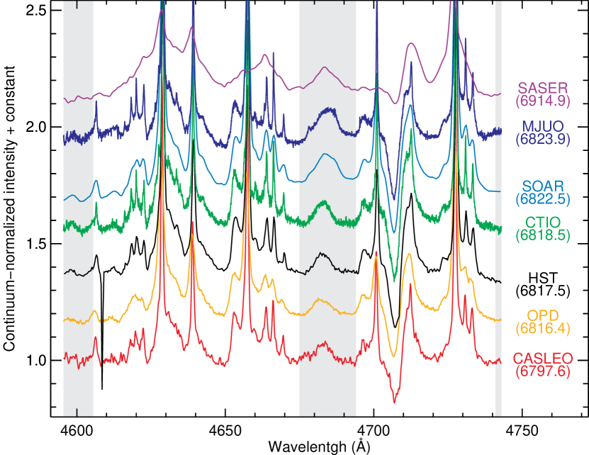
Figure 1.— Typical processed and reduced spectra from collaborators of the campaign. The observatory/team and the date of acquisition (JD-2450000) of the spectrum are indicated on the right side of the figure. Note that, except for the SASER spectrum, which was obtained after the minimum, all of the other spectra were obtained before it and within a timeframe of about 26 d. The vertical shaded regions indicate the regions adopted for continuum (blue: $4600\pm 5$ Å; red: $4742\pm 1$ Å) and line integration ($4675$–$4694$ Å).

2.3. CASLEO/REOSC

Spectral data of $\eta$ Car were also obtained at the Complejo Astronómico El Leoncito (CASLEO), Argentina, from 2014 March through August. The frequency of observations was increased around the periastron passage during 2014 July/August.

The spectra were collected using the reosc spectrograph in its echelle mode, attached to the 2.15-m ‘J. Sahade’ telescope. A Tek $1024\times 1024$ pixel² CCD (24 $\mu$m pixel), was used as detector, providing a dispersion of $0.2$ Å pixel^-1. The wavelength coverage ranges from $4200$ through $6750$ Å.

The normalization of $\eta$ Car spectra was performed by dividing it by the continuum of a hot star, usually $\omega$ Car or $\theta$ Car. Additional residuals were minimized by fitting a low-order polynomial function and defining ad hoc spectral ranges to constrain the continuum to the region $4550$–$4750$ Å.

2.4. HST/STIS

High spatial sampling ($0.05$–$0.1$ arcsec per pixel) spectroscopic mapping of the region was recorded at critical binary orbital phases between 2009 June and 2014 November using the Hubble Space Telescope/Space Telescope Imaging Spectrograph (HST/STIS; see Table 1). The spectra of interest utilized the $52\times 0.1$ arcsec² aperture with the G430M grating centered at $4706$ Å. The mappings were accomplished by a pattern of slit positions centered on $\eta$ Car. While the first two mappings were done at a spacing of $0.1$ arcsec, subsequent mappings were done at $0.05$ arcsec spacing. Allowance for potential detector saturation was provided by a sub-array mapping directly centered on $\eta$ Car. Due to solar panel orientation constraints, the aperture position angle changed between observations. As $\eta$ Car is close to the HST orbital pole, visits were done during continuous viewing zone opportunities, thus increasing observing efficiency more than two-fold. Spatial mappings from these data indicate that the HST/STIS response to the central source have a FWHM=$0.12$ arcsec.

A data cube of flux values was constructed for each spatial position in right ascension and declination at $0.05$ arcsec spacing and in velocity relative to He ii $\lambda 4686$ at 25 km s^-1 intervals ranging from $-8,000$ to $+10,000$ km s^-1.

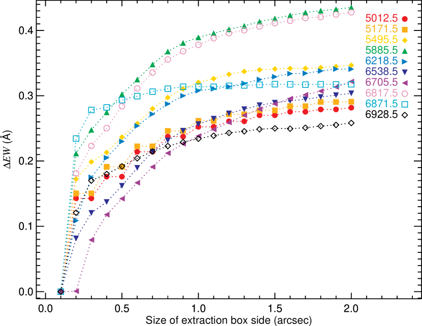
Figure 2.— Aperture correction for the He ii $\lambda 4686$ equivalent width measurements from HST/STIS for each of the 10 visits (the legend indicates ${\rm JD}-2,450,000$ for each visit). The measurements were subtracted by the equivalent width measured within a box region with dimensions $0.1\times 0.1$ arcsec². The larger the extraction aperture, the larger the correction factor to be applied to the HST/STIS measurements in order to compare with the ground-based measurements. The corrected equivalent width, shown in the rest of this paper, is thus given by $EW=EW^{\prime}+\Delta EW$, where $EW^{\prime}$ is the value obtained using an extraction aperture of $0.1\times 0.1$ arcsec².

For the HST/STIS data, the equivalent width of He ii $\lambda 4686$ was measured using the same procedure as for the ground-based observations. However, unlike the space-based observations, emission from the central source cannot be separated from the surrounding nebulosity in ground-based observations due to atmospheric seeing. Hence, direct comparison between the two datasets might be hampered by unwanted contaminations, not only from nebular emission but also from continuum scattered off fossil wind structures (Teodoro et al., 2013). For space-based observations, the contribution from such contaminations is directly proportional to the slit aperture, whereas for ground-based observations, they are always present.

Figure 2 shows that, as we increase the size of the aperture, the amount of He ii $\lambda 4686$ emission relative to the continuum decreases. This indicates that the He ii $\lambda 4686$ emission and adjacent continuum do not come from the same volume. Hence, in order to properly compare the HST/STIS measurements with those obtained by ground-based telescopes, we measured the He ii $\lambda 4686$ equivalent width using the final spectrum obtained from summing up the spectra from the entire $2\times 2$ arcsec² mapping region of the HST/STIS data cube.

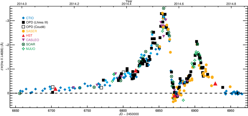
Figure 3.— Equivalent width of He ii $\lambda 4686$. The different symbols and colors identify the contributions from each listed observatory/team. Note that the HST/STIS measurements were obtained using the integrated spectrum within a $2\times 2$ arcsec² region in order to account for the aperture correction required to adequately compare the space- and ground-based measurements. A table containing all the measurements and information about each spectrum is available for download online (see Appendix).

2.5. SOAR/Goodman

The data obtained with the Goodman spectrograph were processed and reduced using standard iraf tasks to correct them for bias and flat-field, as well as to perform the extraction and wavelength calibration of the spectra. For the latter, we used a CuAr lamp to determine a low order (between 3 and 5) Chebyshev polynomial solution for the pixel-wavelength correlation. Observations of a hot standard star (HD 303308; O4 v) were obtained – either just before or following those of $\eta$ Car – in order to correct the spectra by the low frequency distortions caused by instrumental response. The final product was a dataset of spectra with a $SNR$ per resolution element typically in the range from 200 to 1000 (90% of the data) and spectral resolution element of about $85$ km s^-1.

2.6. MJUO/Hercules

Table 3Additional data from the 2009.0 event obtained by R. Chini using the BESO spectrograph on the Hexapod telescope.

JD	EW (Å)	Va (km s-1)
2454846.0	$-0.86\pm 0.10$	$-237.7$
2454851.8	$-0.17\pm 0.10$	$-46.7$
2454871.8	$-0.60\pm 0.10$	$+1.6$
2454874.8	$-0.86\pm 0.10$	$-91.6$
2454877.8	$-0.88\pm 0.10$	$-87.4$
2454882.8	$-1.21\pm 0.10$	$-92.9$
2454887.8	$-0.97\pm 0.10$	$-122.7$
2454891.8	$-0.67\pm 0.10$	$-56.2$
2454896.8	$-0.63\pm 0.10$	$-56.2$
aVelocity of the peak.

Observations for the campaign were taken during 2014 May through 2014 October. The reduction software used was an in-house sequence of packages written using matlab. We typically obtained one to three spectra of $\eta$ Car with exposure time varying between 600 and 1200 s, and one spectrum of the bright hot star $\theta$ Car, with exposure time between 300 and 600 s, depending on sky conditions. The hot star was observed in order to determine the continuum and telluric features for the normalization process. We took a Th-Ar lamp spectrum before and after each science exposure for precise wavelength calibration. Flat-fields were taken at the beginning or end of each night in order to correct the science data for variations on the detector response.

By tracing the orders in the Th-Ar spectral images along the axes defined by the flat fields and using the location of the spectral lines used for wavelength calibration, a full set of wavelength-calibrated axes is obtained along which the stellar orders can be traced. Median filtering was used to remove cosmic rays. The spectral orders of each science image were extracted and merged into a single 1D spectrum.

2.7. SASER

All the data obtained by the members of the Southern Astro Spectroscopy Email Ring (SASER) were fully processed and reduced by them using the standard basic procedure for long slit observations, namely, correction for the bias level and pixel-to-pixel variations, extraction of the spectrum, and wavelength calibration using a comparison lamp. Most of the data were delivered without any continuum normalization. However, they presented variations in intensity within the range $4600$–$4750$ Å that was accounted for by using a linear fit to this region.

2.8. Additional data from the 2009.0 event obtained with HPT/BESO

In this paper, we used 9 additional high resolution ($R\sim 50000$) spectra covering the wavelength range from 3620 to 8530 Å to study the variations in the He ii $\lambda 4686$ strength during the recovery and fading phases after periastron passage. These additional data were obtained with the Bochum Echelle Spectrograph for the Optical (BESO; Fuhrmann et al., 2011) attached to the 1.5 m Hexapod-Telescope (HPT) at the Universitätssternwarte Bochum on a side-hill of Cerro Armazones in Chile. All spectra were reduced with a pipeline based on a MIDAS package adapted from FEROS, the similar ESO spectrograph on La Silla. The results of our measurements for these additional data are listed on Table 3.

3. Results

The high data quality and frequency of observations allowed us to analyze and characterize the variations of the He ii $\lambda 4686$ emission line in unprecedented detail. Figure 3 shows the He ii $\lambda 4686$ equivalent width measurements, EW(He ii $\lambda 4686$), for the entire 2014.6 campaign.

3.1. The period of the spectroscopic cycle derived from the He ii $\lambda 4686$ monitoring

To determine the period of the spectroscopic cycle for He ii $\lambda 4686$, we analyzed the equivalent width measurements using two approaches. (1) We used data encompassing only the last three periastron passages, and then only the data from the interval of sharp decrease in equivalent width prior to the deep minimum. (2) We used the entire equivalent width curve and all datasets, which includes the 1992.4, 2003.5, 2009.0, and 2014.6 events

First, we focused our attention on the decreasing phase of the equivalent width just before the onset of the minimum. During this phase, the equivalent width rapidly decreases from its absolute maximum to a minimum level, which seems to be close to zero. One of the difficulties in assessing the real minimum intensity level is that we need data with both high resolving power and high signal-to-noise, which is not always available for a long-term dedicated monitoring. Also, small variations in the spectrum induced by data processing, reduction, and/or normalization of the spectra are the major contributors to stochastic fluctuations during the minimum intensity phase.

We noted that, as opposed to 2003.5 and 2009.0, the decreasing phase for the 2014.6 periastron passage did not occur at a linear rate. Therefore, instead of adopting the methodology used by Damineli et al. (2008a) for the disappearance of the narrow component of the He i $\lambda 6678$ line, we used the approach suggested by Mehner et al. (2011). This method consists in finding the minimum ($EW_{\mathrm{min}}$) and maximum ($EW_{\mathrm{max}}$) value for the equivalent width during periastron passage, ignoring the time when they occur. Then, the mid-point is determined by $EW_{\mathrm{m}}=(EW_{\mathrm{min}}+EW_{\mathrm{max}})/2$. Next, the observed equivalent width that is nearest to $EW_{\mathrm{m}}$ is found, for which the corresponding time, JD($EW_{\mathrm{m}}$), is taken as reference. Applying this procedure to consecutive periastron passages allows us to determine the period by calculating the difference between JD($EW_{\mathrm{m}}$)’s. Figure 4 illustrates this methodology and shows the results for data from the last three events (2003.5, 2009.0, and 2014.6). The mean period obtained by using this approach was $2022.9\pm 0.2$ d, where the uncertainty is the standard deviation of the mean (the standard error is $0.14$ d).

We also used the entire curve (including all the observations from 1992.4 up to 2014.6) to determine the period for the He ii $\lambda 4686$. We folded the equivalent width curve using trial periods to determine which period would result in the least dispersion of the data. This method, called phase dispersion minimization (PDM; Stellingwerf, 1978), is frequently used to search for periodic signals in the light curve of eclipsing binary systems. In this work, we adopted the Plavchan algorithm (Plavchan et al., 2008), which is a variant of the PDM method. The Plavchan algorithm folds the light curve to trial periods and, for each period, computes the $\chi^{2}$ difference between the original and the box-car smoothed data, but only for a predefined number of worst-fit subset of the data. Thus, the best period is the one that produces the lowest $\chi^{2}$ value.

Using the Periodogram Service available at the NASA Exoplanet Archive, we tested a sample of 300 trial periods, equally distributed between 2010 and 2040 d. The number of elements of the worst-fit subset was set to 50 and we adopted a smoothing box-car size of 0.01 in phase. With these parameters, the result of the analysis using the Plavchan algorithm is shown in Figure 5a.

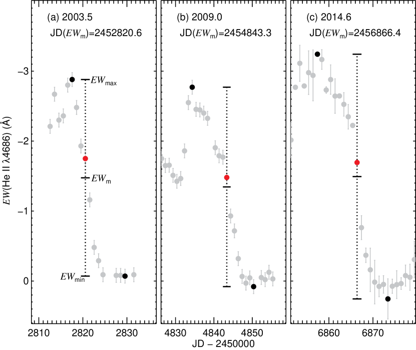
Figure 4.— Period determination using the equivalent width of He ii $\lambda 4686$ around periastron passage for the last 3 events: (a) 2003.5, (b) 2009.0, and (c) 2014.6. The two black dots in each panel indicate the observed maximum and minimum $EW$(He ii $\lambda 4686$), from where the mean equivalent width, $EW_{\mathrm{m}}$, was determined. The red dot indicates the observation nearest to $EW_{\mathrm{m}}$, whereas the vertical dotted line indicates the corresponding time of the observation, JD($EW_{\mathrm{m}}$), indicated on the top of each panel. The period was then determined as the mean of the differences $2014.6-2009.0$ and $2009.0-2003.5$. The mean period of the He ii $\lambda 4686$ obtained by this method was $2022.9\pm 0.2$ d.

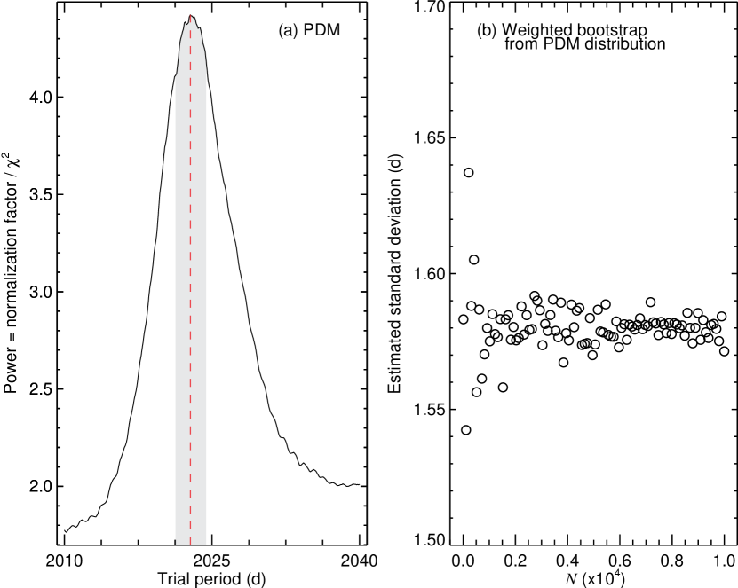
Figure 5.— (a) He ii $\lambda 4686$ period determination using phase dispersion minimization analysis (PDM) of the entire dataset covering the 5 last events (1992.4, 1998.0, 2003.5, 2009.0, and 2014.6). The analysis was performed using the Plavchan period-finding algorithm, resulting in a period of $2022.8$ d. The standard deviation of the mean (shaded area in (a)) was estimated by using a weighted bootstrap technique, suggesting a value of $\pm 1.58$ d.

Table 4Period of the spectroscopic cycle determined by different methods (adapted from Damineli et al. 2008a).

Method	Perioda (d)
$V$ band	$2021\pm 2$
$J$ band	$2023\pm 1$
$H$ band	$2023\pm 1$
$K$ band	$2023\pm 1$
$L$ band	$2023\pm 2$
Fe ii $\lambda 6455$ P Cyg radial velocity	$2022\pm 2$
He i $\lambda 6678$ broad comp. radial velocity	$2022\pm 1$
Si ii $\lambda 6347$ EW	$2022\pm 1$
Fe ii $\lambda 6455$ P Cyg EW	$2021\pm 2$
He i $\lambda 6678$ narrow comp. EW	$2026\pm 2$
He i $\lambda 10830$ EW	$2022\pm 1$
X-ray light curve (1992–2014)	$2023.5\pm 0.7$
He ii $\lambda 4686$ EW (1992–2014)	$2022.9\pm 1.6$
Weighted mean $\pm$ standard error	$2022.7\pm 0.3$
aThe error is the standard deviation of the mean.

The maximum of the PDM power distribution, which corresponds to the minimum $\chi^{2}$, occurred for a period of $2022.8$ d. Although the uncertainty associated with this result cannot be obtained directly from the PDM analysis, an estimate of the standard deviation of the mean can be determined by using a weighted bootstrap technique with resampling, where a random sample with a predefined size is drawn from the original period dataset (in this case, within the range $2010$–$2040$ d). The probability of drawing a given period was determined by the PDM distribution itself and we restricted the size of each drawn sample to be 75% the size of the original dataset. Repeating this procedure $N$ times, where $N\rightarrow\infty$, allows us to obtain an estimate of the true standard deviation of the mean. Figure 5b shows that this method rapidly converges: for $N\gtrsim 5000$ the dispersion of the results is about 1%, suggesting a standard deviation of the mean of about $\pm 1.6$ d.

The results from the two methods described in this section are consistent and can be used to obtain a mean period of $2022.9\pm 1.6$ d.

3.2. Reassessing the mean period of the spectroscopic cycle and its uncertainty

As an update to the previous work by Damineli et al. (2008a), we used the new result from He ii $\lambda 4686$ in combination with previous period determinations in order to obtain a mean period of the spectroscopic cycle. Table 4 lists some of the methods used to determine the period. That table is an adapted version of table 2 from Damineli et al. (2008a), which now includes an updated value for the period determined from the X-ray light curves, including data from 1992–2014 (Corcoran et al., in preparation), and the new determination from the He ii $\lambda 4686$ equivalent width (from 1992–2014).

The weighted mean period was determined by a two-step approach. First, an unweighted mean of the 13 periods listed in Table 4 was determined. Then, a new mean was determined by weighting each period by its absolute difference regarding the unweighted mean. This approach has the benefit of not being so sensitive to discrepant measurements, which has a great impact on the uncertainties in the period determination.

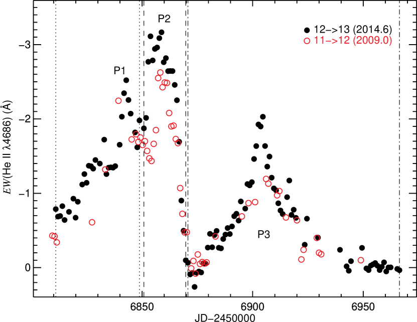
Figure 6.— Comparison between the equivalent width of He ii $\lambda 4686$ around periastron passage for the 2014.6 event (black filled circles) and that of 2009.0, shifted by 2022.8 d (red open circles). The vertical lines delimit the time interval used to check for variability in P1 (dotted lines), P2 (dashed lines), and P3 (dash-dotted lines) separately.

The result suggests a weighted mean period for the spectroscopic cycle of $2022.7\pm 0.3$ d, where the error is the standard error of the mean (the standard deviation is $0.9$ d). Thus, the mean period has not changed with the new measurements, but its uncertainty has considerably been reduced. Evidently, this improvement was mainly due to the fact that we adopted a weighted approach to the period determination, and not because we included an updated measurement from X-rays and a new datum from He ii $\lambda 4686$.

3.3. The recurrence of the EW curve

We tested the hypothesis that the overall distribution of the equivalent width of the He ii $\lambda 4686$ around the event is recurrent, i.e., it comes from the same distribution. We limited our analysis to the past two events (2009.0 and 2014.6) because they were monitored over almost one year (centered on the event) at a relatively high time sampling.

The period obtained from the He ii $\lambda 4686$ equivalent width was used to fold the observed curve of the 2009.0 event by 2022.9 d in order to compare it with the recent 2014.6 event. Three non-parametric statistical tests were employed to address the similarities between the equivalent width curves from 2009.0 and 2014.6: the Anderson-Darling $k$-sample test (Scholz & Stephens, 1987; Knuth, 2011), the two-sample Wilcoxon test (also known as Mann-Whitney test; Hollander & Wolfe, 1973; Bauer, 2012), and the Kolmogorov-Smirnov test (Birnbaum & Tingey, 1951; Conover, 1971; Durbin, 1973; Marsaglia et al., 2003). We used the R package R Core Team (2014) to perform the statistical analysis.

All of the statistical tests used here are non-parametric, which means that they make no assumption on the intrinsic distribution of the samples under comparison. The null hypothesis, $H_{0}$, for these tests is that the samples come from the same parent distribution. The tests return a parameter, called test statistic ($T_{\rm obs}$), which is then compared with a critical value ($T_{\rm c}$) that is calculated based on the size of the samples and on the chosen significance level, $\alpha$. Thus, the null hypothesis is rejected at the significance level $\alpha$ if $T_{\rm obs}\geq T_{\rm c}$, which is known as the traditional method. Another equally valid approach is to calculate the probability, under the null hypothesis, of getting a $T$ as large as $T_{\rm obs}$, which is called the $p$-value method. In this case, the $p$-value must be compared to the chosen significance level, $\alpha$, and the null hypothesis is rejected when $p(T\geq T_{\rm c})\leq\alpha$. For the analysis presented here, we established a significance level of $\alpha=0.05$, and we always discard $H_{0}$ whenever one of the two methods rejects the null hypothesis.

Figure 6 shows the equivalent width curve (ranging from JD = 2454787.5 through 2454926.0 for 2009.0 and from JD = 2456810.96 through 2456966.37 for the 2014.6 curve) for which we performed these statistical analyses. Table 5 indicates that both conditions, $T_{\rm obs}\leq T_{\rm c}$ and $p(T\geq T_{\rm c})\geq\alpha$, are true for all tests performed on the entire curve, suggesting that we cannot reject the null hypothesis. Note that, under the assumption that the null hypothesis is valid, a value of $p(T\geq T_{\rm c})\geq 0.1$ is classified as weak evidence against the null hypothesis at the significance level $\alpha=0.05$, whereas $p(T\geq T_{\rm c})\geq 0.2$ is considered as no evidence against the null hypothesis (Fisher, 1925, 1935). Thus, the results of the analysis for the entire curve suggest that there is only weak evidence of significant changes in the He ii $\lambda 4686$ equivalent width from one cycle to another.

Table 5Results of the two-sample statistical analysis, performed on the equivalent width curve of 2009.0 and 2014.6 (Figure 6), to test for the null hypothesis ($H_{0}$) that the two curves have the same distribution. $T_{\rm obs}$ is the test statistic and $p(T\geq|T_{\rm obs}|)$ is the probability, assuming that $H_{0}$ is valid, of obtaining a test statistic as extreme as observed. $N_{1}$ and $N_{2}$ are the sample size for 2009.0 and 2014.6, respectively.

Hypothesis test	$|T_{\rm obs}|$	$T_{\rm c}$a	$p(T\geq|T_{\rm obs}|)$	Reject $H_{0}$?
Entire curve ($N_{1}=54$ and $N_{2}=122$)
ADb	0.156	1.960	0.300	No
Wrsc	0.626	1.960	0.532	No
KSd	0.127	0.222	0.583	No
P1 only ($N_{1}=11$ and $N_{2}=32$)
AD	1.041	1.960	0.120	No
Wrs	0.334	1.960	0.738	No
KS	0.364	0.475	0.229	No
P2 only ($N_{1}=20$ and $N_{2}=20$)
AD	6.195	1.960	0.001	Yes
Wrs	3.00	1.960	0.003	Yes
KS	0.600	0.430	0.002	Yes
P3 only ($N_{1}=23$ and $N_{2}=70$)
AD	-0.021	1.960	0.365	No
Wrs	0.045	1.960	0.964	No
KS	0.199	0.327	0.501	No
aCritical value of the test for a significance level $\alpha=0.05$.
bAD: Anderson-Darling test.
cWrs: Wilcoxon rank sum test.
dKS: Kolmogorov-Smirnov test.

We also looked for changes in the intensity of each peak (P1, P2, and P3) separately. For this, we defined three data subsets, each one containing one peak, to be analyzed in the same way as the entire curve. The first subset, containing P1, is composed of data within the range 2454787.5–2454826.36 for 2009.0 and within 2456810.96–2456848.81 for 2014.6. The second subset, which contains P2, is composed of data within 2454827.36–2454846.29 for 2009.0 and within 2456850.81–2456869.74 for 2014.6. Finally, the third subset contains P3 and is composed of data within 2454847.29–2454926 for 2009.0 and within 2456870.73–2456966.37 for 2014.6.

The results shown in Table 5 suggest that P1 and P3 did not change significantly between 2009.0 and 2014.6. In contrast, P2 had a statistically significant increase in strength over this period; the mean difference between the two epochs is about 0.53 Å, which corresponds to a relative increase of about 26% from 2009.0 to 2014.6.

Caution is advised regarding the lack of variability of P1 and P3, since their different sample size (resulting from different frequencies of observations) might have some influence on the statistical analysis in the case where significant changes occurred during epochs not covered by the monitoring. Since P2 does not suffer from different sampling between 2009.0 and 2014.6, the result obtained for this peak is more reliable than that for P1 and P3. Nevertheless, even if we adopt a different time interval to be used for the statistical analyses of each peak (e.g. reducing the time interval for P3 to the range 2456880–2456935), the outcome of the tests remain unchanged. Therefore, our results suggest that P3 might be composed of a broad and a narrow component. The former has been detected in previous events, but the latter was only detected in 2014.6 due to the better time sampling of observations. Further discussion on this discrepancy in P3 between 2009.0 and 2014.6 is presented in Section 5.

3.3.1 Comparing equivalent width measurements from HST/STIS and ground-based

There has been a debate about discrepancies resulting from measuring the equivalent width of the He ii $\lambda 4686$ using HST/STIS and ground-based observations. Recently, Davidson et al. (2015), based on five measurements using HST/STIS data, suggested that the He ii $\lambda 4686$ equivalent width for the 2014.6 event was systematically different from the past cycles. Their conclusion relies on the direct comparison between HST/STIS and ground-based observations for the past two cycles (2009.0 and 2014.6).

In the case of $\eta$ Car, HST/STIS observations have undoubtedly higher quality than the ground-based ones in the sense that they allow us to obtain the spectrum of the central source with relatively less contamination from the surrounding nebulosities. Nevertheless, space-based observations could not be scheduled so as to have the same time coverage possible from the ground, which were performed almost on a daily basis (at least around the event, for the past two cycles). Also, ground-based optical spectra frequently are obtained with a much higher resolving power than possible with HST/STIS, allowing us to have better understanding of the line morphologies.

Thus, it is a good practice to compare the data obtained with HST/STIS with those obtained from ground-based telescopes. However, for the reasons mentioned in Section 2.4, aperture corrections must be applied to the measurements obtained from space-based telescopes in order to be properly compared with the ground-based measurements. This correction must be performed by summing up the observed equivalent width and the aperture correction factor obtained from Figure 2. Figure 7 shows the result of performing such corrections to the measurements published in Davidson et al. (2015). The amount of correction for each measurement was determined from our HST/STIS data using the closest observation. After the corrections were applied, no significant differences are observed (within the uncertainties of the measurements).

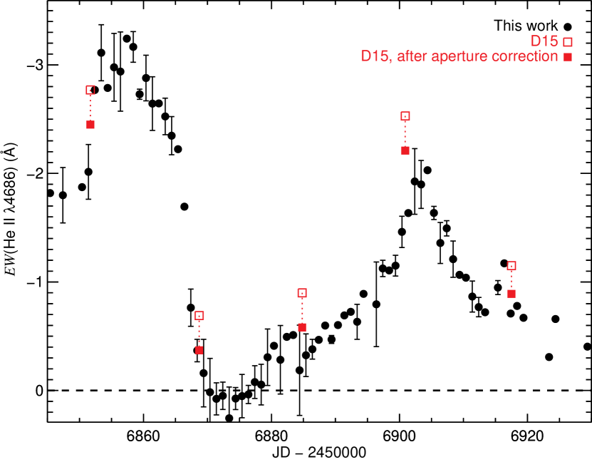
Figure 7.— Comparison between the measurements presented in this work for the 2014.6 event (using ground- and space-based telescopes) and those from Davidson et al. (2015, D15, using HST/STIS observations), before (red open squares) and after (red solid squares) applying aperture corrections to their measurements.

Although we did not detect significant variations in the overall behavior of the equivalent width curve of the He ii $\lambda 4686$ equivalent width in a timeframe of 5.54 yr, we cannot discard the possibility of changes over longer timescales. However, this can only be adequately addressed by continuously monitoring $\eta$ Car over several more cycles.

3.4. Detection of He ii $\lambda 4686$ emission around apastron

A comparison between the He ii $\lambda 4686$ line profile at phases around apastron and periastron is shown in Figure 8. That figure leaves no doubt about the positive detection of this line in emission at phases around apastron for the last cycle (between 2009.0 and 2014.6). Indeed, as can be seen from Figure 8a, there is a noticeable hump in the range from 4675 to 4694 Å, where the He ii $\lambda 4686$ is located at phases around periastron. As an illustration of what a zero He ii $\lambda 4686$ emission would look like, Figure 8b shows two spectra taken at the onset of the He ii $\lambda 4686$ deep minimum (2014 Jul 31), using CTIO/CHIRON and HST/STIS data. The region where the He ii $\lambda 4686$ line was previously detected is flat, showing no evident line profile.

Due to the restricted wavelength interval adopted to calculate the He ii $\lambda 4686$ equivalent width (4675–4694 Å), contamination from the broad component of the iron emission lines on both sides of the integration region are always included in the measurements at all phases. This effect can be especially significant at phases around apastron, when the intensity of the He ii $\lambda 4686$ line is relatively low and contaminations become stronger.

Although we cannot reliably determine the exact magnitude of the contaminations, we can estimate a minimum value for the He ii $\lambda 4686$ equivalent width at apastron by reducing the size of the integration region so that we keep only the observed line profile. As can be seen in Figure 8a, the He ii $\lambda 4686$ line profile is evident in the range 4679–4691 Å (shaded area in that figure). The equivalent width measured within this reduced region, at apastron, was about $-0.051$ Å for SOAR and $-0.048$ Å for HST/STIS, resulting in a minimum of $-0.05\pm 0.01$ Å. For the sake of completeness, the equivalent width measured within the wider wavelength interval (4675–4694 Å) was $-0.083$ Å for SOAR and $-0.075$ Å for HST/STIS, which implies an equivalent width of $-0.08\pm 0.01$ Å. Hence, the minimum equivalent width of the He ii $\lambda 4686$ emission line at apastron is $-0.07\pm 0.01$ Å.

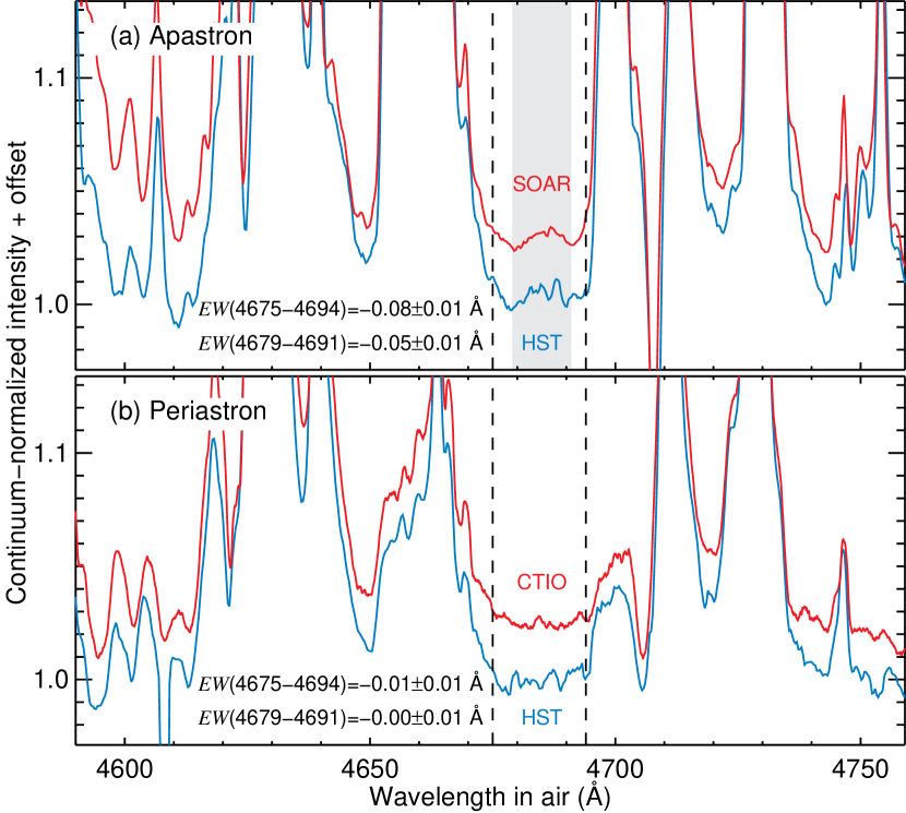
Figure 8.— Ground- and space-based spectra taken at phases around (a) apastron and (b) periastron, showing the consistency of the equivalent width ($EW$) measured in both data. For clarity, the ground-based spectra were shifted vertically by an offset of $0.025$. The vertical dashed lines indicate the wavelength interval from 4675–4694 Å, usually adopted for the equivalent width determination, whereas the shaded region indicates the range 4679–4691 Å, which was adopted at apastron in order to minimize the contribution from the wings of the neighboring iron lines to the flux within the integration region. The $EW$ indicated in each panel is the minimum value for each wavelength interval. See main text for more details.

4. Discussion

The phase-locked behavior of the overall He ii $\lambda 4686$ equivalent width curve (including P1, P2, and P3; see Figure 9a) suggests that at least the bulk of the line strength is due to non-stochastic processes occurring at phases close to periastron passages. However, due to intricate changes in the line profile, it is not clear yet where such a large amount of He ii $\lambda 4686$ emission is located, how extended it is, nor how the line emission mechanism changes with time. Nevertheless, our results have the potential to shed light on the dominant mechanism behind the changes in the He ii $\lambda 4686$ equivalent width curve.

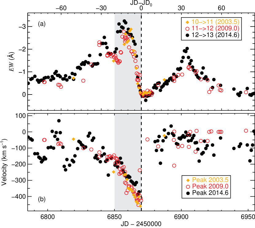
Figure 9.— (a) He ii $\lambda 4686$ equivalent width curve for the last three events folded by $2022.9$ d. (b) Doppler velocity measurements. The shaded region indicates the period where the peak velocity rapidly changes to more blue-shifted velocities, which repeated for the past three events. This kinematic behavior seems to be related only with P2.

There is a consensus that, at least during periastron passages, He ii $\lambda 4686$ emission should be produced close to the WWC region, most likely in the dense, cool, pre-shock primary wind (Martin et al., 2006; Teodoro et al., 2012; Madura et al., 2013). This is in agreement with the fact that the observed maximum Doppler velocity of the peak of the line profile is $400\lesssim|V|\lesssim 450$ km s^-1 (see Figure 9b), which is comparable to the primary wind terminal velocity of 420 km s^-1 (Groh et al., 2012a). This region is also favored by arguments related to the energy required to produce the observed line luminosity, as extensively discussed in previous works (e.g. Martin et al., 2006; Mehner et al., 2011; Teodoro et al., 2012). Thus, in general, any feasible scenario for the He ii $\lambda 4686$ production around periastron passage requires that the emitting region is adjacent to the wind-wind collision shock cone, close to its apex. This is the basic assumption for the model we propose next.

4.1. A model for the variations in the He ii $\lambda 4686$ equivalent width curve: opacity and geometry effects.

Assuming that the He ii $\lambda 4686$ emission is produced close to the apex of the shock cone, variations in the observed emission can, in principle, be explained by the increase in the total opacity along the line of sight to the emitting region, as the secondary moves deeper inside the dense primary wind. Intuitively, this mechanism would cause a gradual decrease (or increase, after periastron passage) of the observed flux that would depend on the extent and physical properties of the optically thick region in the extended primary wind, and also on the orbital orientation to the observer.

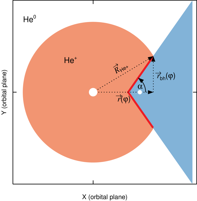
Figure 10.— Sketch (not to scale) of the intersection between the wind-wind interacting region (represented by a cone) and the He⁺ region (represented by the orange circle) at phases around periastron. When the stars (white circles) are close enough, so that the wind-wind interacting region penetrates the He⁺ core in the primary wind, high-energy radiation produced in the shock cone (red line) can easily ionize He⁺ ions, and some of the radiation due to the eventual recombination processes will escape through the aperture of the ‘bore hole’. This will lead to an increasing in the production of He ii $\lambda 4686$ photons.

This same approach was used by Okazaki et al. (2008) to show that the overall behavior of the RXTE X-ray light curve can be reproduced by assuming that the X-ray emission comes from a point source located at the apex of the shock cone and prone to attenuation by the primary wind. Recently, Hamaguchi et al. (2014) suggested that the variations across the spectroscopic events are composed of a combination of (1) occultation of the X-ray emitting region by the extended primary wind and (2) decline of the X-ray emissivity at the apex. In any case, opacity effects (either attenuation or occultation) can play an important role on the observed intensity of the radiation. Since the X-ray light curve shares some similarities with the He ii $\lambda 4686$ equivalent width curve (both rise to a maximum before falling to a minimum when there is no emission at all), we tested the hypothesis that the variations in the He ii $\lambda 4686$ equivalent width could also be the result of intrinsic emission attenuated by the extended primary wind.

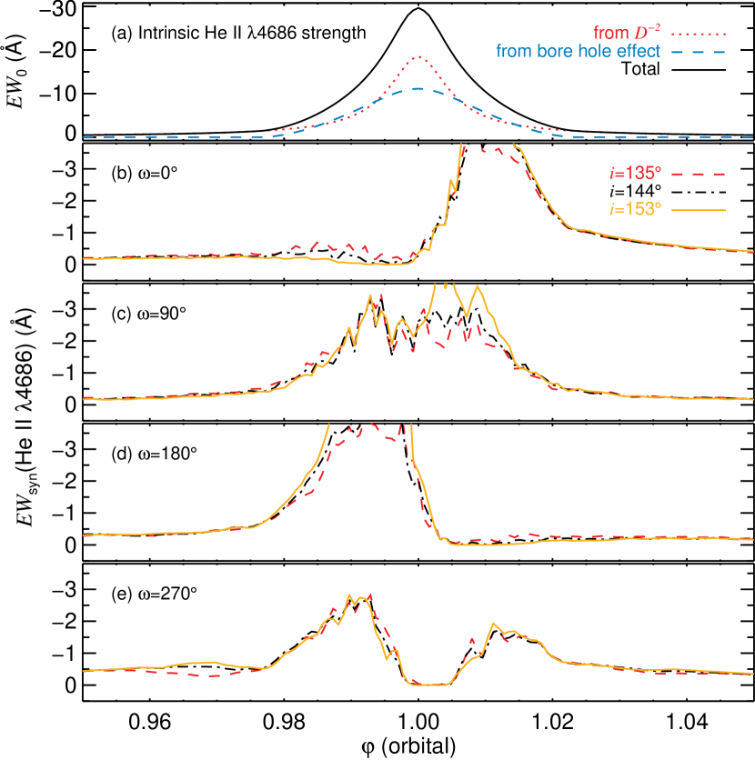
Figure 11.— (a) Intrinsic and (b–e) synthetic He ii $\lambda 4686$ equivalent width curves. The basic assumption is that the He ii $\lambda 4686$ emission comes from a region located at the apex and varies accordingly to the total column density in the line of sight to it as derived from 3D SPH simulations ($D$ is the distance between the stars). The same intrinsic line strength was assumed for all orbit orientations. For each value of the longitude of periastron ($\omega$), the different lines show the expected behavior of the equivalent width for the orbit inclinations ($i$) indicated in the legend. Variations in the equivalent width curve are more sensitive to $\omega$ than $i$. Based on these plots and the observations, we can promptly exclude $0\arcdeg\lesssim\omega\lesssim 180\arcdeg$ and favor $\omega$ close to $270\arcdeg$.

We used 3D SPH simulations of $\eta$ Car from Madura et al. (2013) to calculate the total optical depth in the line of sight to the apex at each phase by using

$$\tau_{\rm A}(\varphi)=\kappa_{e}\,\int_{z_{0}(\varphi)}^{R}\rho\,dz,$$ (1)

where $\rho$ and $\kappa_{e}$ are, respectively, the mass density and the mass absorption coefficient of the material in the line of sight to the apex. The integration starts at the position of the apex at each phase $z_{0}(\varphi)$ and goes up to the boundaries of the 3D SPH simulations, which, in this case, is a sphere with radius $R=154.5$ AU. For the present work, we assumed that electron scattering is the dominant process for the attenuation of the radiation in the line of sight, which corresponds to $\kappa_{e}=0.34$ cm² g^-1. Therefore, under these circumstances, the synthetic equivalent width, $EW_{\rm syn}$, at each orbital phase, was obtained using

$$EW_{\rm syn}(\varphi)=EW_{0}(\varphi)\,e^{-\tau_{\rm A}(\varphi)},$$ (2)

where $EW_{0}(\varphi)$ is the intrinsic equivalent width (corresponding to the unattenuated flux). In the present work, we included only two mechanisms responsible for $EW_{0}$: (i) a continuous production of He ii $\lambda 4686$ photons that varies reciprocally with the square of the distance $D$ between the stars (i.e. in radiative conditions; see Fahed et al., 2011) and (ii) an additional, temporary contribution from the ‘bore hole’ effect that depends on how deep the apex of the shock cone penetrates inside the primary wind (see Madura & Owocki, 2010).

We included the contribution from the ‘bore hole’ effect because, near periastron, due to the highly eccentric orbit, the wind-wind interacting region penetrates into the inner regions of the primary wind, eventually exposing its He⁺ core. The contribution from this mechanism to the observed He ii $\lambda 4686$ flux is proportional to how large the ‘bore hole’ is (see Figure 10). This assumption relies on the fact that high-energy radiation produced in the shock cone inside the He⁺ region (the red line between the cone and the sphere in Figure 10) can create He⁺⁺ ions, whose recombination will produce He ii $\lambda 4686$ photons. Some will eventually escape through the ‘bore hole’ and be detected by the observer.

The radius $r_{\rm bh}$ of the ‘bore hole’ is wavelength-dependent and varies with orbital phase. Considering the He⁺ region, $r_{\rm bh}$ as a function of the orbital phase is given by

$$r_{\rm bh}(\varphi)=(R^{2}_{\rm He^{+}}-r^{2}(\varphi))^{1/2},$$ (3)

where $r(\varphi)$ is the distance between the primary star and the plane formed by the aperture of the ‘bore hole’ (see Figure 10), given by

$$r(\varphi)=\frac{c^{2}\,z_{0}(\varphi)+(c^{2}\,(R^{2}_{\rm He^{+}}-z^{2}_{0}(\varphi))+R^{2}_{\rm He^{+}})^{1/2}}{c^{2}+1},$$ (4)

and $c=\tan\alpha$, where $\alpha$ is the half-opening angle of the cone formed by the wind-wind interacting region. In equations 3 and 4, $R_{\rm He^{+}}$ is the radius of the He⁺ region in the primary wind and $z_{0}(\varphi)$ is the distance between the primary and the apex at a given orbital phase. Figure 11a shows the contribution from each mechanism to the total intrinsic equivalent width $EW_{0}$. The relative contribution was chosen so that the transition between the two regimes occurred smoothly, as required by the observations. Thus, by combining the intrinsic strength for the line emission with the total opacity in the line of sight, we were able to calculate a synthetic equivalent width curve for different orbit orientations. The results for selected orbital orientations are shown in Figure 11b–e.

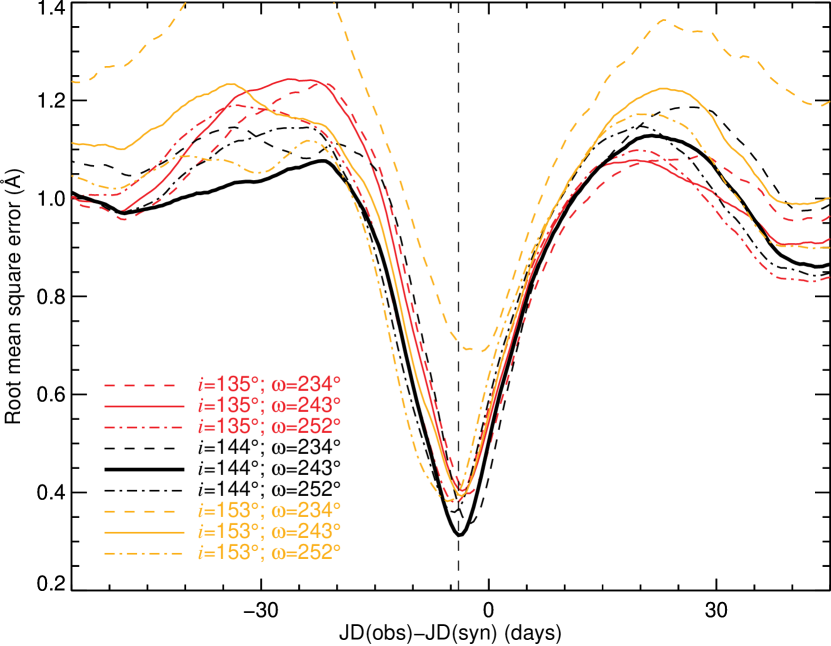
Figure 12.— Examples of the result of the comparison between the observed He ii $\lambda 4686$ equivalent width curve and a series of synthetic curves from 3D SPH simulations with different orbital orientations (3 inclinations and 3 longitude of periastron). For each comparison, we shifted the models in time to determine the time of periastron passage. Each curve shows the least root mean square error as a function of the difference between the time of the observations, JD(obs), and that of the synthetic equivalent width curve, JD(syn), for the indicated orbit orientation. The best match occurred for $i=144\arcdeg$, $\omega=243\arcdeg$ (black solid line), and a time shift of about $-4.0$ d.

4.2. Modeling the He ii $\lambda 4686$ equivalent width

4.2.1 The direct view of the central source

Based on the comparison between the overall profile of the observed He ii $\lambda 4686$ equivalent width curve from the past 3 cycles and those synthetic curves shown in Figure 11, one can readily discard models with $0\arcdeg\lesssim\omega\lesssim 180\arcdeg$. Orientations with $\omega=0\arcdeg$ produce results that have excessively high optical depths before periastron passage and way too little after it. This orientation cannot reproduce the observed rise of the equivalent width before periastron passage and also overestimates its strength after it. Orientations with $\omega=90\arcdeg$ produce symmetrical profiles, which do not correspond to the observations. Orientations with $\omega=180\arcdeg$ can reproduce fairly well the observations before periastron but fail to reproduce the observed equivalent width after periastron (they underestimate P3).

Regardless of the overall profile of the synthetic equivalent width curves, the crucial problem of models with $0\arcdeg\lesssim\omega\lesssim 180\arcdeg$ is that they cannot reproduce the observed phase of the deep minimum – the week-long phase where the observed equivalent width is zero.

Orientations with $230\arcdeg\lesssim\omega\lesssim 270\arcdeg$, on the other hand, seem to provide a good overall profile, as they predict an increase just before periastron passage followed by a rapid decrease to zero right after periastron passage, and the return to a lower (in modulo) equivalent width peak before fading away (P3). Thus, we focused our analysis on $\omega$ in this range.

The duration of the interval when the synthetic equivalent width remains near zero (and whether it is ever reached) is also regulated by the orbital inclination. Thus, we compared the observations with 16 synthetic equivalent width curves obtained from the permutation of 4 values of orbital inclination ($i\in\{126\arcdeg,135\arcdeg,144\arcdeg,153\arcdeg\}$) and 5 values of longitude of periastron ($\omega\in\{225\arcdeg,234\arcdeg,243\arcdeg,252\arcdeg,261\arcdeg\}$). Then we calculated the root mean square error (RMSE) between each model and the observations. The values for $i$ and $\omega$ were obtained from a pre-defined grid within the 3D SPH models. Also, note that the orbital plane is parallel to the plane of the sky for $i=0\arcdeg$ or $i=180\arcdeg$, whereas for $i=90\arcdeg$ or $i=270\arcdeg$ they are perpendicular to each other. Thus, the set of orbital inclinations that we investigated in this work was chosen based on the premise that the orbital axis is aligned with the Homunculus polar axis (see Madura et al., 2012).

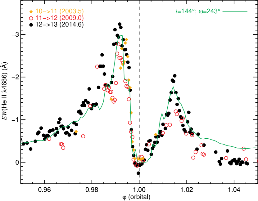
Figure 13.— Folded He ii $\lambda 4686$ equivalent width curve compared with the best synthetic model (solid green line). The minimum RMSE occurs when the synthetic model is shifted by $-4.0$ d relative to the observations. Note that now the phase corresponds to the orbital phase.

For each model, we also searched for the time shift to be applied to the models that would result in the least root mean square value between the model and the observations. Examples of the results of this analysis are shown in Figure 12. The minimum RMSE was reached for an orbit orientation with {$i=144\arcdeg$, $\omega=243\arcdeg$} and a time shift $\mathrm{JD(obs)}-\mathrm{JD(syn)}=-3.5$ d. A comparison between the best model (with the derived time shift applied) and the observations is shown in Figure 13.

Regarding the mean value and uncertainty of these results, statistical analysis showed that there are no significant differences between a model with a combination of $i=144\arcdeg$ and $234\arcdeg\lesssim\omega\lesssim 252\arcdeg$. In fact, within the range of orbit orientations that we focused our analysis on, only these models resulted in RMSE significantly lower than the others at the $2\sigma$ level. Therefore, the mean values we adopted for $i$ and $\omega$ are, respectively, $144\arcdeg$ and $243\arcdeg$ (coincidently equal to the best match), whereas the uncertainty on both values is defined by the step in the number of lines of sight used to produce the synthetic equivalent width curves from the 3D SPH models, which was set to $9\arcdeg$. In order to estimate the mean and uncertainty on the time shift, we adopted a sample composed of the time shift that resulted in the least RMSE for each one of the 16 models. The result was a mean time shift of $-4.0\pm 2.0$ d (the standard error is $\pm 0.5$ d). This means that periastron passage occurs 4 d after the onset of the He ii $\lambda 4686$ deep minimum.

4.2.2 The event as viewed from high stellar latitudes

An independent way to verify the reliability of our results would be analyzing the He ii $\lambda 4686$ equivalent width curve from different viewing angles and comparing them with the results from the direct view of the central source. Fortunately, in the case of $\eta$ Car, this is possible due to the bipolar reflection nebula – the Homunculus nebula – that surrounds the binary system. Each position along the Homunculus nebula ‘sees’ the central source along a different viewing angle (Smith et al., 2003b). An interesting position is the FOS4 (e.g. Davidson et al., 1995; Humphreys & HST-FOS eta Car Team, 1999; Zethson et al., 1999; Rivinius et al., 2001; Stahl et al., 2005), a region about $1$ arcsec² in area located approximately 4.5 arcsec from the central source along the major axis of the Homunculus that is believed to reflect the spectrum originating at stellar latitudes close to the polar region (for comparison, the spectrum from the direct view of the central source seems to arise from intermediate stellar latitudes; see e.g. Smith et al., 2003b).

We compared our results with those obtained at FOS4 by Mehner et al. (2015) using the same analysis that we did for the direct view of the central source. Note, however, that the time shift obtained from the observations at FOS4 needs to be corrected by the light travel time and the expansion of the reflecting nebula. We achieved this by using the Homunculus model derived by Smith (2006), to determine the necessary parameters of FOS4 (see Figure 14). In a coordinate system where a stellar latitude of $\theta=90\arcdeg$ corresponds to the pole of the receding NW lobe and $\theta=270\arcdeg$ corresponds to the pole of the approaching SE lobe, the spectrum reflected at FOS4 corresponds to a stellar latitude of $\theta({\rm FOS4})=258\arcdeg$, whereas the central source is viewed at $\theta_{0}=229\arcdeg$.

Figure 15 shows the search for the best match between the models and the observations. Since the orbital axis is closely aligned with the Homunculus polar axis, we investigated models corresponding to stellar latitudes $\theta\in\{252\arcdeg,261\arcdeg,270\arcdeg\}$ and $\omega\in\{225\arcdeg,243\arcdeg,252\arcdeg\}$. The best match was found for {$\theta=261\arcdeg$, $\omega=243\arcdeg$} and a time shift of $-21.0$ d. This model resulted in a RMSE significantly lower (at the $2\sigma$ level) than any other one. Note that this time shift of 21 d, obtained empirically Smith (2006), is consistent with previous estimates by Stahl et al. (2005) and Mehner et al. (2011) based on geometrical arguments.

Since the observations at FOS4 were not as frequent as for the direct view, our analysis is subject to aliasing, which explains the high frequency oscillations observed in Figure 15. Despite that, we determined a mean time shift at FOS4 of $-21.6\pm 1.3$ d (the standard error is $0.4$ d). Note that the smaller uncertainty of this result, when compared with the direct view of the central source, is not real. This is just an effect introduced by the fact that we used a smaller sample for the trial models for the polar region than for the direct view. Also, the variations between the trial models for the polar region are not as large as the ones for the direct view, which reduces the dispersion of the minimum RMSE (all the models for the pole region have similar time shift).

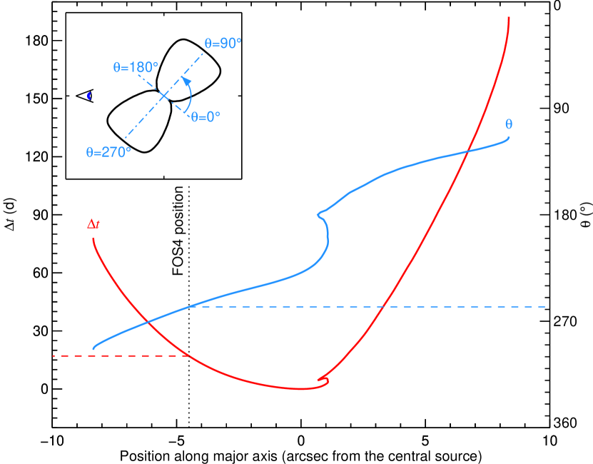
Figure 14.— Time delay ($\Delta t$) and stellar latitude ($\theta$) as a function of the projected position along the major axis of the Homunculus nebula. The inset illustration shows the the definition of the stellar latitude regarding the orientation of the Homunculus nebula. Values between $0\arcdeg$ and $180\arcdeg$ correspond to the NW lobe ($\theta=90\arcdeg$ being the NW pole), whereas latitudes between $180\arcdeg$ and $360\arcdeg$ correspond to the SE lobe ($\theta=270\arcdeg$ is the SE pole). In this system, the direct view of the central source corresponds to $\theta\equiv\theta_{0}=229\arcdeg$. The vertical dotted line indicates the FOS4 position, whereas the horizontal dashed lines indicate the corresponding values for $\Delta t=17$ d (left vertical axis) and $\theta=258\arcdeg$ (right vertical axis).

The time shift we derived for FOS4 has to be corrected by light travel delay. Considering that the lobes are expanding at $650$ km s^-1, the spectrum reflected at the FOS4 position would be delayed by $\Delta t=17$ d relative to the direct view of the central source. This means that $17$ d, out of the observed $-21.6$ d, are due to light travel effect that must be taken into account in order to compare with the observations of the central source (again, the minus sign means periastron occurs after the onset of the He ii $\lambda 4686$ deep minimum). Therefore, the best model for the observations at FOS4 results in an effective time shift of $17$ d$-21.6$ d$=-4.6\pm 0.4$ d, which is in agreement with the results obtained from the direct view of the central source. Figure 16 shows the best model compared with the observations at FOS4 (corrected for light travel time). An interesting result is that when the ‘bore hole’ effect is included, the models overestimate the equivalent width at FOS4, which suggests that the contributions due to this mechanism is small at high stellar latitudes. This makes sense, given the fact that the contribution from the ‘bore hole’ effect will be significant toward where the cavity is pointing to (i.e. low and intermediate latitudes).

The net result is that the ephemeris equation derived from the reflected observations at FOS4 (high stellar latitude), after correction by the travel time delay, is the same as for the direct view (intermediate stellar latitude). Therefore, the variations across the event for the He ii $\lambda 4686$ seem to be ultimately determined by the high opacity in the line of sight to the He ii $\lambda 4686$ emitting region during periastron passage, and not by a decrease in the intrinsic emission.

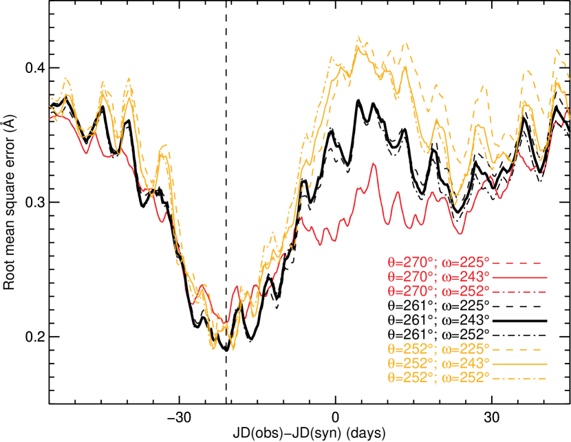
Figure 15.— Same as Figure 12, but for the position FOS4. At this position, we are looking at a spectrum originated at a stellar latitude $\theta$ that is being reflected off the Homunculus nebula. In this system, $\theta=90\arcdeg$ corresponds to the NW lobe pole, whereas $\theta=270\arcdeg$ corresponds to the SE lobe pole. The best match (black solid line) occurred for $\theta=261\arcdeg$, $\omega=243\arcdeg$, and a time shift of $-21.0$ d.

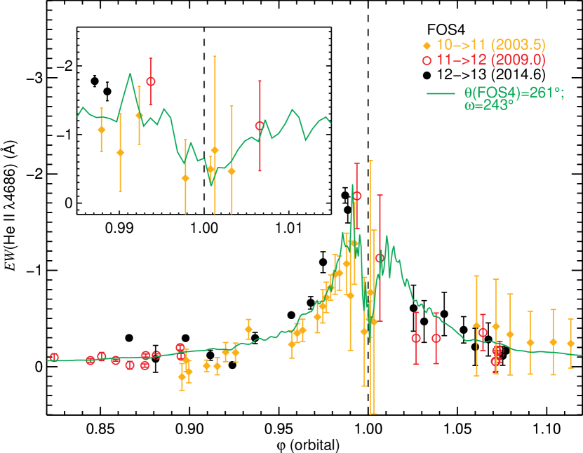
Figure 16.— FOS4 observations from Mehner et al. (2015) corrected by the time delay ($17$ d). The green solid line corresponds to the best match model: $\theta({\rm FOS4})=261\arcdeg$ and $\omega=243\arcdeg$. The vertical dashed line indicates periastron passage.

4.3. Ephemeris equation for periastron passage

The results presented in this paper allowed us to determine the time of the periastron passage, $T_{0}(2014.6)$, from two different line of sights. For the direct view, $T_{0}(2014.6)=2456874.1$ (standard deviation: $\pm 2.8$ d), whereas for the FOS4 $T_{0}(2014.6)=2456874.7$ (standard deviation: $\pm 2.3$ d). Therefore, the time of periastron passage is given by

$${\rm JD(periastron~{}passage)}=2456874.4+2022.7\,E,$$ (5)

where $E=(\Phi-13)$, $\Phi$ is the mean anomaly plus cycle, and $2022.7$ corresponds to the mean period of the spectroscopic cycle. The time of periastron passage determined by equation 5 has an uncertainty of $\pm 2.0$ d (standard error), which is the result of error propagation from all the parameters used to determine the mean values shown in that equation. Table 6 summarizes all the orbital elements derived in this work and Figure 17 illustrates the orientation of the orbit projected onto the sky using the mean value for the orbital elements.

4.4. The He ii $\lambda 4686$/X-ray connection

The comparison between the He ii $\lambda 4686$ emission and the X-rays is inevitable because both are tracers of high-energy processes that might be interconnected. For example, X-rays produced in the wind-wind shock might be used to doubly-ionize neutral helium, in which case the He ii $\lambda 4686$ emission should vary in a similar way to the X-rays.

In $\eta$ Car, the onset of the deep minimum, as determined from the observed He ii $\lambda 4686$ and $2$–$10$ keV X-ray emission light curves, occurs almost at the same time (see e.g. Teodoro et al., 2012; Hamaguchi et al., 2014). Incidentally, no significant changes in the time of the start of the deep minimum were observed over the past 3 cycles (Corcoran et al. 2016, in preparation). However, the recovery of the He ii $\lambda 4686$ emission and the $2$–$10$ keV X-ray flux occurs in a completely different way. So far, the observations support a scenario where the He ii $\lambda 4686$ emission presents a recovery phase (after the deep minimum) that is stable and repeatable, whereas for the X-rays, recovery cannot be predicted. Indeed, in 1998.0 and 2003.5, the full recovery of the $2$–$10$ keV X-ray flux occurred about 90 d after the onset of the deep minimum, but in 2009.0 it happened 30 d earlier than that. Even more intriguing, in 2014.6, the observations indicate that the recovery was intermediate between the 1998.0/2003.5 and 2009.0. Thus, the question is why does the He ii $\lambda 4686$ and the X-ray emission enter the deep minimum at the same time but recover from it so differently? Are they connected?

Hamaguchi et al. (2014) showed that the $2$–$10$ keV X-ray flux can be split into two regimes that behave differently in time: the soft (2–4 keV) and the hard X-ray band (4–8 keV). Those authors showed that the hard X-ray flux (4–8 keV) drops to a minimum before the soft X-ray flux (2–4 keV). In fact, by the time the latter reaches the minimum, the former is already recovering from it. Interestingly, He ii $\lambda 4686$ emission enters the minimum phase about 4 d after the hard X-rays and about 12 d before the soft X-rays. This fact not only corroborates the idea that the He ii $\lambda 4686$ emitting region is located in the vicinity of the apex (likely close to the hard X-ray emitting region), but is also consistent with the scenario proposed in this paper, in which the onset of the deep minimum is regulated by the orbital orientation and opacity effects, as the secondary moves toward periastron. In this scenario, emission from the apex should disappear first, followed by emission produced in regions gradually farther away from the WWC apex (i.e., downstream of the WWC structure). Therefore, the time when the deep minimum starts should be approximately the same for all features arising from spatially adjacent regions, as might be the case for He ii $\lambda 4686$ and the X-rays (especially the hard band flux).

Table 6Orbital elements derived in the present work, assuming orbital eccentricity $\epsilon=0.9$.

Parameter	Symbol	Value or range
Inclination	$i$	$135\arcdeg$–$153\arcdeg$
Longitude of periastron	$\omega$	$234\arcdeg$–$252\arcdeg$
Period	$P$	$2022.7\pm 0.3$a
Time of periastron passage	$T_{0}$(2014.6)	$2456874.4\pm 1.3$a
aThe error is the standard error of the mean.

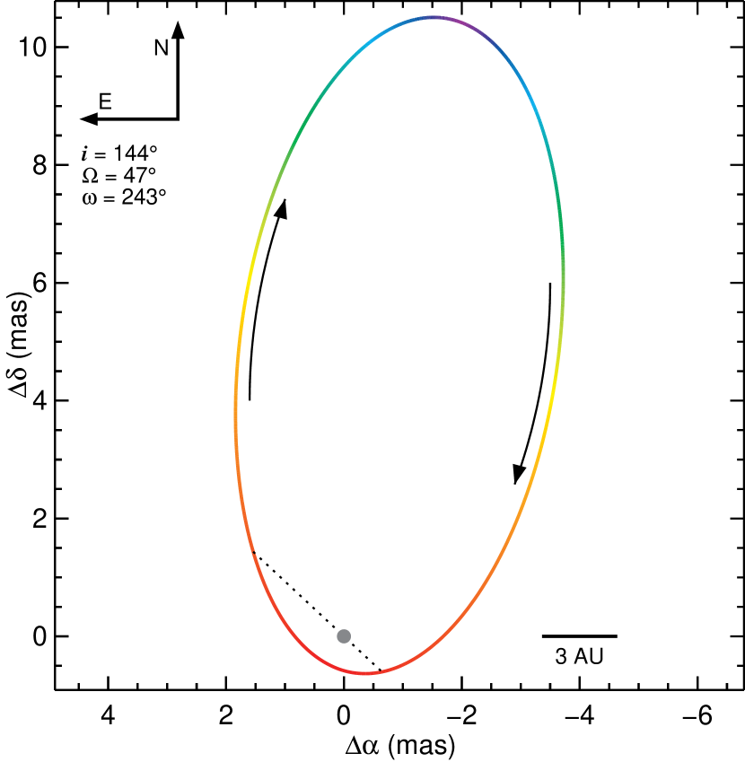
Figure 17.— Orientation of the orbit of the secondary star as projected onto the sky using the mean value of the orbital elements derived in the present work. The arrows indicate the direction of the orbital motion. Note that the orbit is with respect to the primary star. The orbit was color-coded using the actual (not projected) distance between the stars, so that the orbit path becomes red as the stars are close to each other around periastron passage, and purple when they are at apastron. We adopted a distance of $2350$ pc Smith (2006).

Using the ephemeris from Hamaguchi et al. (2014), the deep minimum phase in the hard X-rays occurred, approximately, from $\mathrm{JD}=2454843$ through $\mathrm{JD}=2454859$, which suggests that superior conjunction would have occurred within this interval. According to equation 5, the 2009.0 periastron passage occurred on $\mathrm{JD}=2454851.7$, which falls approximately in the middle of the phase of minimum hard X-ray flux. Moreover, note that, for $\omega=243\arcdeg$, superior conjunction occurs very close to periastron passage, only 3.6 d later. Therefore, the orbital orientation as derived from X-ray and He ii $\lambda 4686$ emission are consistent. This is not surprising in the scenario we propose here. Indeed, close to periastron passages, we expect the hard X-ray and the He ii $\lambda 4686$ to behave similarly (although they might not have a causal relation) because the apex of the shock cone is inside the primary He⁺ core where the He ii $\lambda 4686$ emission is being produced at these phases. The soft X-rays, however, are produced in extended regions along the shock cone, and will eventually be blocked by the inner dense parts of the primary star at a later time.

After periastron passage, the He ii $\lambda 4686$ emission behaves differently from the X-rays likely due to intrinsic physical processes that inhibit or even shut off the latter, but not the former. For example, if the shock cone structure would switch from adiabatic to radiative during periastron passage, the result would be a substantial decrease of the hardest X-ray emission because the wind-wind interacting region would be cooler. The subsequent recovery of the X-ray emission would then depend on stochastic processes in order to re-establish the emission from the hot plasma in the wind-wind interaction region. This is not, however, the case for the He ii $\lambda 4686$ emission because, during periastron passage, the He⁺ region of the primary star is exposed by the wind-wind interacting region, and, therefore, He ii $\lambda 4686$ emission can still be produced during this phase, even if there is very low X-ray emission from the WWC region.

5. Final remarks

Analysis of the data we have thus far indicate that only P2 has significantly increased in strength over the past two cycles (2009.0 and 2014.6). This is a robust result because we have daily measurements during the appearance of P2 for those epochs. However, except during the 2014.6 periastron passage, P1 and P3 have never been monitored with high cadence, which makes the comparison rather difficult because the equivalent width of the He ii $\lambda 4686$ line shows variations at a wide range of timescales.

One clear example is the absolute maximum strength of P3. The results from the 2009.0 analysis (including the additional data obtained with Hexapod/BESO) suggest that it is composed of a broad peak with a maximum absolute value of about $1.3$ Å, but the 2014.6 results indicate that P3 is actually a combination of broad and sharp components, with a maximum absolute value of $2$ Å. The broad component does repeat from cycle to cycle, but we cannot conclude the same for the narrow component, as we did not have enough time coverage during the time the narrow component seems to appear. Nonetheless, a caveat here is that short-timescale variations (less than a week) might occur due to local stochastic mechanisms, like the flares seen in X-rays before periastron passages. Such fluctuations cannot be easily distinguished from cyclic variations.

Our model is especially sensitive to two parameters: (i) the total opacity in the line of sight to the apex and (ii) to the size of the He⁺ region in the primary wind. Hence, changes in these parameters will reflect on the overall behavior of the He ii $\lambda 4686$ equivalent width curve. As a matter of fact, both parameters are ultimately connected to the mass-loss rate of the primary star. Changes in the primary’s mass-loss rate would result in variations in the timing and strength of the He ii $\lambda 4686$ equivalent width curve (as already discussed in Madura et al., 2013). The repeatability of the overall behavior of the He ii $\lambda 4686$ equivalent width over the past three cycles, as shown in this work, corroborates previous results that rule out large changes in mass-loss rate from the primary star over that time interval.

6. Conclusions

We have monitored the He ii $\lambda 4686$ emission line across the 2014.6 event using many ground-based telescopes as well as the HST. The main results derived from the analysis of the collected data are listed below.

• The period of $2022.9\pm 1.6$ d, derived from He ii $\lambda 4686$ monitoring, is in agreement with previous results;

• Based on several different measurements across the electromagnetic spectrum, the mean orbital period is $2022.7\pm 0.3$ d;

• We have not detected statistically significant changes in the overall behavior of the He ii $\lambda 4686$ equivalent width curve when comparing the events of 2009.0 and 2014.6 (best time sampled), which implies that the mechanism behind the production of EUV/soft X-rays photons must be relatively stable and recurrent;

• When comparing each peak separately, between 2009.0 and 2014.6, P1 and the broad component of P3 have not changed significantly. Nevertheless, P2 has increased by 26%;

• We have proposed a model to explain the variations of the He ii $\lambda 4686$ equivalent width curve across each event. The model assumes two different mechanisms responsible for the intrinsic production of the line emission: (1) a component that is inversely proportional to the square of the distance between the two stars (always present throughout the orbit) and (2) another one associated with the ‘bore hole’ effect (present within about $30$ d before and $30$ d after periastron passage; negligible outside this time interval). The intrinsic emission was then convolved with the total optical depth in the line of sight to the He ii $\lambda 4686$ emitting region (computed from 3D SPH simulations) to create a synthetic equivalent width that was compared with the observations;

• Our model was able to successfully reproduce the overall behavior of the He ii $\lambda 4686$ equivalent width curve from two very different viewing angles: a direct view and a polar view of the central source. The latter was possible due to observations from the FOS4 position on the SE lobe of the Homunculus nebula. This particular position is known for its capability of reflecting the spectrum of the central source produced at high stellar latitudes;

• The best match between the models and observations from two different viewing angles (direct view of the central source and FOS4) suggests $234\arcdeg\lesssim\omega\lesssim 252\arcdeg$;

• We have determined the time of periastron passage by comparing the time shift required to give the best match between models (for which we know the orbital phase) and observations for two different lines of sight. The results suggest that both directions ‘see’ the periastron passage at the same time, about $4$ d after the start of the deep minimum (as seen in the direct view of the central source);

In summary, our results suggest that the variations observed in the He ii $\lambda 4686$ equivalent width curve across the spectroscopic events are governed by a combination of the orbit orientation regarding the observer and the total optical depth in the line of sight to the emitting region. This is not a classical eclipse of the emitting region by the primary wind (the so-called ‘wind eclipse’ scenario). Instead, the ultimate nature of the spectroscopic event can be ascribed to the deep burial of the secondary star in the densest parts of the primary wind, so that emission from the vicinity of the apex of the shock cone cannot easily escape the system, resulting in a temporary decrease of the observed emission regardless of line of sight.

As a reminder, the onset of the next He ii $\lambda 4686$ deep minimum will occur on 2020 February 13. Periastron passage should occur four days later.

Table 7 lists all the 2014.6 measurements presented in this paper, as well as information about the quality and wavelength coverage of each spectrum used.

Table 7He ii $\lambda 4686$ emission line measurements and spectral characteristics of the data obtained during the international campaign to monitor the 2014.6 periastron passage.

	$EW$	Velocity of			Wavelength
JD-2450000		the peak	$\Delta\mathrm{v\tablenotemark{a}}$	SNR	coverage	Observatory
	(Å)	(km s-1)	(km s-1)		(Å)
4967.47314	$+0.16\pm 0.08$	$-10$	185.7	1579	3499–6168	SOAR
4978.45698	$+0.16\pm 0.08$	$-28$	185.8	1079	3497–6167	SOAR
5012.50000	$+0.03\pm 0.03$	$-678$	39.5	955	4560–4826	HST
5171.50000	$+0.20\pm 0.03$	$-678$	39.5	629	4560–4826	HST
5495.50000	$+0.35\pm 0.03$	$-678$	39.5	334	4560–4826	HST
5689.50746	$-0.23\pm 0.08$	$-23$	92.5	350	3509–4839	SOAR
5729.53926	$+0.06\pm 0.08$	$+522$	92.1	342	3516–4841	SOAR
5768.49673	$+0.12\pm 0.08$	$+514$	92.0	353	3517–4840	SOAR
5856.82809	$+0.08\pm 0.08$	$+526$	92.0	307	3517–4839	SOAR
5885.50000	$+0.16\pm 0.03$	$-678$	39.5	272	4560–4826	HST
5893.79688	$-0.24\pm 0.08$	$-668$	92.1	396	3509–4832	SOAR
5930.77193	$-0.06\pm 0.08$	$-59$	92.0	379	3513–4836	SOAR
5955.81938	$+0.14\pm 0.08$	$-672$	92.0	250	3518–4841	SOAR
5982.61373	$+0.11\pm 0.08$	$+526$	91.9	346	3517–4839	SOAR
5989.68923	$+0.01\pm 0.13$	$+530$	3.5	640	4505–4755	CTIO
5993.75221	$+0.04\pm 0.13$	$+530$	3.5	620	4505–4755	CTIO
6001.72621	$+0.08\pm 0.13$	$+530$	3.5	678	4505–4755	CTIO
6003.63393	$+0.05\pm 0.08$	$+514$	92.0	287	3518–4840	SOAR
6013.68632	$+0.22\pm 0.13$	$-684$	3.5	594	4505–4755	CTIO
6039.52767	$+0.02\pm 0.08$	$+525$	92.2	422	3511–4836	SOAR
6079.49884	$+0.03\pm 0.08$	$+515$	92.1	299	3519–4843	SOAR
6116.49641	$-0.13\pm 0.08$	$+530$	92.0	279	3521–4844	SOAR
6136.46326	$+0.08\pm 0.08$	$+527$	92.2	289	3515–4841	SOAR
6218.50000	$+0.22\pm 0.03$	$-358$	39.5	368	4560–4826	HST
6221.89057	$+0.20\pm 0.13$	$+530$	3.5	584	4505–4755	CTIO
6236.84632	$-0.06\pm 0.13$	$-684$	3.5	548	4505–4755	CTIO
6238.87015	$-0.04\pm 0.13$	$-684$	3.5	410	4505–4755	CTIO
6246.79354	$+0.01\pm 0.08$	$+521$	92.0	323	3517–4839	SOAR
6248.81477	$-0.10\pm 0.13$	$+530$	3.5	606	4505–4755	CTIO
6254.88181	$-0.19\pm 0.13$	$-684$	3.5	558	4505–4755	CTIO
6260.78284	$-0.05\pm 0.13$	$+530$	3.5	433	4505–4755	CTIO
6275.81899	$+0.28\pm 0.13$	$-684$	3.5	673	4505–4755	CTIO
6278.81225	$+0.26\pm 0.08$	$+518$	92.0	333	3516–4839	SOAR
6289.79792	$+0.16\pm 0.13$	$-684$	3.5	788	4505–4755	CTIO
6346.69729	$+0.09\pm 0.08$	$-673$	91.9	439	3520–4841	SOAR
6361.58149	$-0.24\pm 0.08$	$+526$	91.9	327	3518–4839	SOAR
6361.64473	$+0.12\pm 0.13$	$+530$	3.1	742	4505–4755	CTIO
6401.58757	$-0.07\pm 0.13$	$+530$	3.1	772	4505–4755	CTIO
6417.58964	$-0.09\pm 0.13$	$+530$	3.1	675	4505–4755	CTIO
6428.48444	$-0.03\pm 0.08$	$+522$	92.3	460	3511–4837	SOAR
6428.64093	$-0.03\pm 0.13$	$+131$	3.8	2046	4575–4800	CTIO
6452.52706	$-0.05\pm 0.08$	$+31$	92.2	357	3514–4840	SOAR
6488.47634	$-0.19\pm 0.08$	$+14$	91.9	484	3516–4838	SOAR
6538.50000	$+0.10\pm 0.03$	$-17$	39.5	265	4560–4826	HST
6607.84573	$+0.12\pm 0.13$	$+530$	3.1	497	4505–4755	CTIO
6612.86785	$-0.22\pm 0.13$	$+324$	3.1	577	4505–4755	CTIO
6613.83605	$-0.34\pm 0.08$	$+15$	91.1	420	3632–4941	SOAR
6655.76290	$+0.01\pm 0.15$	$-1$	47.2	615	6398–6720	SOAR
6656.70393	$-0.09\pm 0.08$	$-30$	3.1	1225	4283–4961	CTIO
6659.70988	$-0.08\pm 0.13$	$-29$	3.1	690	4505–4755	CTIO
6664.67479	$-0.17\pm 0.13$	$+530$	3.1	607	4505–4755	CTIO
6670.78253	$-0.01\pm 0.13$	$-31$	3.1	657	4505–4755	CTIO
6672.83764	$-0.04\pm 0.13$	$-71$	3.1	766	4505–4755	CTIO
6677.75915	$-0.17\pm 0.13$	$+12$	3.1	625	4505–4755	CTIO
6687.70761	$-0.10\pm 0.13$	$-37$	3.1	755	4505–4755	CTIO
6690.69063	$-0.18\pm 0.13$	$-6$	3.1	800	4505–4755	CTIO
6697.72572	$-0.27\pm 0.08$	$-2$	3.1	743	4505–4755	CTIO
6698.77338	$-0.17\pm 0.08$	$+55$	3.7	1814	4505–4755	CTIO
6701.62899	$-0.03\pm 0.13$	$+10$	99.7	399	4575–4800	OPD (Lhires iii)
6701.74483	$-0.26\pm 0.03$	$+136$	46.1	184	4571–5052	OPD (Coudé)
6705.50000	$-0.18\pm 0.03$	$+22$	39.5	374	4396–4894	HST
6710.66775	$-0.10\pm 0.03$	$+14$	3.1	911	4560–4826	CTIO
6712.69246	$-0.23\pm 0.13$	$-7$	3.1	614	4505–4755	CTIO
6718.70977	$-0.15\pm 0.13$	$-45$	3.1	680	4505–4755	CTIO
6724.59005	$-0.22\pm 0.13$	$-11$	3.7	1944	4505–4755	CTIO
6725.56888	$-0.12\pm 0.13$	$-103$	3.1	700	4575–4800	CTIO
6729.55975	$-0.23\pm 0.13$	$-126$	3.0	946	4505–4755	CTIO
6730.60581	$-0.23\pm 0.15$	$+527$	26.6	655	6399–6720	CASLEO
6732.60351	$-0.20\pm 0.13$	$-111$	3.0	899	4505–4755	CTIO
6739.49790	$-0.22\pm 0.13$	$-42$	91.3	934	4540–4760	SOAR
6739.54616	$-0.22\pm 0.13$	$-42$	3.1	828	4505–4755	CTIO
6746.51736	$-0.39\pm 0.35$	$-37$	3.1	628	3627–4940	CTIO
6750.53884	$-0.30\pm 0.13$	$+2$	3.1	642	4505–4755	CTIO
6754.55102	$-0.31\pm 0.13$	$-44$	3.1	702	4505–4755	CTIO
6759.52573	$-0.25\pm 0.13$	$-17$	91.4	486	4505–4755	SOAR
6763.55612	$-0.33\pm 0.13$	$-36$	29.1	1082	4505–4755	CASLEO
6765.58734	$-0.40\pm 0.35$	$+7$	3.0	878	3625–4940	CTIO
6766.54334	$-0.25\pm 0.13$	$-61$	3.1	987	4540–4760	CTIO
6767.50868	$-0.35\pm 0.13$	$+14$	3.1	908	4505–4755	CTIO
6769.52337	$-0.23\pm 0.13$	$-1$	46.1	517	4505–4755	OPD (Coudé)
6772.43126	$-0.54\pm 0.13$	$-73$	100.1	201	4505–4755	OPD (Lhires iii)
6774.54408	$-0.33\pm 0.13$	$-152$	3.1	784	4461–4959	CTIO
6775.46760	$-0.53\pm 0.13$	$+28$	3.7	1968	4571–5055	CTIO
6777.53611	$-0.45\pm 0.13$	$+71$	3.7	1819	4505–4755	CTIO
6781.47143	$-0.31\pm 0.13$	$-105$	3.1	911	4575–4800	CTIO
6784.84146	$-0.49\pm 0.13$	$-33$	3.2	1252	4575–4800	MJUO
6786.50087	$-0.56\pm 0.13$	$-43$	3.7	2346	4505–4755	CTIO
6786.80812	$-0.78\pm 0.08$	$-43$	3.2	1041	4586–4818	MJUO
6787.50338	$-0.62\pm 0.13$	$-46$	3.7	1774	4575–4800	CTIO
6787.80222	$-0.80\pm 0.08$	$-54$	3.2	1390	4586–4817	MJUO
6789.57938	$-0.80\pm 0.13$	$-135$	26.5	519	4575–4800	CASLEO
6791.55016	$-0.63\pm 0.08$	$-135$	3.1	1017	4586–4817	CTIO
6793.39493	$-0.57\pm 0.13$	$-159$	100.2	585	4540–4760	OPD (Lhires iii)
6793.43162	$-0.52\pm 0.13$	$-153$	100.2	260	4505–4755	OPD (Lhires iii)
6793.51309	$-0.61\pm 0.13$	$-163$	26.5	1712	4569–5053	CASLEO
6795.44909	$-0.63\pm 0.13$	$-185$	100.3	114	4569–5053	OPD (Lhires iii)
6795.44909	$-0.63\pm 0.13$	$-185$	100.3	114	4540–4760	OPD (Lhires iii)
6795.50702	$-0.72\pm 0.13$	$-174$	3.1	971	4570–5055	CTIO
6796.46794	$-0.52\pm 0.13$	$-175$	93.7	1262	4570–5055	SOAR
6796.66742	$-0.72\pm 0.13$	$-158$	100.3	103	4505–4755	OPD (Lhires iii)
6797.51150	$-0.80\pm 0.35$	$-159$	100.3	564	3593–4940	OPD (Lhires iii)
6797.56402	$-0.69\pm 0.13$	$-174$	26.5	462	4565–5049	CASLEO
6800.41794	$-0.87\pm 0.13$	$-93$	46.9	433	4556–5040	OPD (Coudé)
6800.46206	$-0.65\pm 0.13$	$-102$	3.1	838	4540–4760	CTIO
6801.49770	$-0.64\pm 0.13$	$-94$	3.1	737	4035–5176	CTIO
6802.50447	$-0.79\pm 0.13$	$+3$	3.7	1702	4505–4755	CTIO
6803.52719	$-0.70\pm 0.13$	$-100$	3.1	1034	4505–4755	CTIO
6805.46847	$-0.93\pm 0.13$	$-27$	100.3	388	4575–4800	OPD (Lhires iii)
6805.48993	$-1.01\pm 0.13$	$-4$	100.3	275	4505–4755	OPD (Lhires iii)
6806.52963	$-0.84\pm 0.13$	$-46$	3.7	460	4568–5052	CTIO
6807.61259	$-0.85\pm 0.13$	$+68$	3.7	490	4568–5052	CTIO
6809.45843	$-0.79\pm 0.13$	$-4$	3.7	2494	4575–4800	CTIO
6810.48189	$-0.69\pm 0.13$	$-94$	3.1	868	4575–4800	CTIO
6811.48702	$-0.79\pm 0.13$	$-260$	3.7	2121	4575–4800	CTIO
6812.45066	$-0.60\pm 0.13$	$-166$	99.3	151	4505–4755	OPD (Lhires iii)
6813.40174	$-0.76\pm 0.13$	$-239$	99.9	567	4575–4800	OPD (Lhires iii)
6813.42771	$-0.89\pm 0.13$	$-230$	99.9	193	4574–5054	OPD (Lhires iii)
6814.41074	$-0.66\pm 0.13$	$-176$	99.9	732	4573–5056	OPD (Lhires iii)
6814.43755	$-0.62\pm 0.13$	$-165$	99.9	186	4573–5056	OPD (Lhires iii)
6816.43650	$-0.73\pm 0.13$	$-205$	99.8	393	4573–5055	OPD (Lhires iii)
6816.43650	$-0.77\pm 0.13$	$-207$	99.8	280	4573–5055	OPD (Lhires iii)
6817.50000	$-0.94\pm 0.13$	$-178$	39.5	359	4573–5055	HST
6818.42255	$-0.91\pm 0.13$	$-174$	99.8	233	4573–5055	OPD (Lhires iii)
6818.50425	$-0.67\pm 0.03$	$-185$	3.1	888	4560–4826	CTIO
6820.41744	$-0.89\pm 0.13$	$-148$	102.4	546	4587–5069	OPD (Lhires iii)
6821.80127	$-1.09\pm 0.13$	$-67$	3.2	901	4505–4755	MJUO
6822.38703	$-1.14\pm 0.13$	$-136$	102.4	525	4577–5055	OPD (Lhires iii)
6822.45982	$-1.32\pm 0.22$	$-106$	91.2	2197	4586–4818	SOAR
6823.45482	$-1.20\pm 0.13$	$-58$	99.9	522	4577–5055	OPD (Lhires iii)
6823.53806	$-1.12\pm 0.35$	$-68$	3.1	772	3626–4938	CTIO
6823.86265	$-1.16\pm 0.13$	$-62$	3.2	960	4575–5057	MJUO
6824.51692	$-1.47\pm 0.13$	$-58$	3.1	1085	4505–4755	CTIO
6825.44362	$-1.27\pm 0.22$	$-89$	99.9	719	4589–4818	OPD (Lhires iii)
6825.46968	$-1.26\pm 0.13$	$-90$	99.9	379	4505–4755	OPD (Lhires iii)
6825.50553	$-1.59\pm 0.13$	$-68$	3.7	2021	4574–5057	CTIO
6826.42638	$-1.30\pm 0.13$	$-104$	99.9	924	4574–5057	OPD (Lhires iii)
6826.45073	$-1.30\pm 0.13$	$-83$	99.9	339	4575–4800	OPD (Lhires iii)
6826.85107	$-1.37\pm 0.13$	$-74$	3.2	886	4574–5057	MJUO
6827.40873	$-1.42\pm 0.13$	$-113$	99.9	835	4575–5057	OPD (Lhires iii)
6827.43762	$-1.21\pm 0.22$	$-107$	99.9	622	4586–4818	OPD (Lhires iii)
6827.77608	$-1.51\pm 0.13$	$-119$	3.2	1263	4574–5057	MJUO
6828.40903	$-1.38\pm 0.13$	$-67$	102.4	602	4574–5057	OPD (Lhires iii)
6829.50184	$-1.57\pm 0.22$	$-42$	3.1	481	4586–4818	CTIO
6830.39501	$-1.31\pm 0.13$	$-11$	99.9	637	4577–5055	OPD (Lhires iii)
6830.39501	$-1.32\pm 0.13$	$-23$	99.9	660	4505–4755	OPD (Lhires iii)
6831.47240	$-1.72\pm 0.13$	$-8$	91.3	411	4575–5057	SOAR
6832.50051	$-1.43\pm 0.13$	$-32$	3.1	908	4575–5057	CTIO
6833.37832	$-1.15\pm 0.35$	$-63$	99.9	800	3626–4938	OPD (Lhires iii)
6833.37832	$-1.20\pm 0.13$	$-60$	99.9	238	4505–4755	OPD (Lhires iii)
6833.50054	$-1.34\pm 0.13$	$-38$	3.7	1941	4574–5057	CTIO
6835.36656	$-1.35\pm 0.13$	$-159$	102.4	615	4574–5057	OPD (Lhires iii)
6835.53378	$-1.17\pm 0.13$	$-132$	3.1	489	4575–4800	CTIO
6836.36515	$-1.52\pm 0.13$	$-159$	102.4	997	4577–5055	OPD (Lhires iii)
6836.49685	$-1.33\pm 0.13$	$-149$	3.1	758	4505–4755	CTIO
6837.38253	$-1.40\pm 0.13$	$-184$	100.0	1368	4577–5055	OPD (Lhires iii)
6838.51346	$-1.65\pm 0.13$	$-196$	3.7	1813	4505–4755	CTIO
6839.46217	$-1.86\pm 0.13$	$-172$	100.0	395	4576–5058	OPD (Lhires iii)
6839.50001	$-1.98\pm 0.13$	$-169$	3.7	2037	4575–4800	CTIO
6840.45062	$-2.25\pm 0.13$	$-149$	100.0	360	4576–5059	OPD (Lhires iii)
6840.46309	$-2.53\pm 0.13$	$-124$	91.3	1422	4575–4800	SOAR
6840.49851	$-2.43\pm 0.13$	$-121$	3.7	2212	4575–5059	CTIO
6841.39145	$-2.08\pm 0.35$	$-73$	100.2	350	3627–4939	OPD (Lhires iii)
6842.43257	$-2.52\pm 0.13$	$-136$	102.4	1203	4575–4800	OPD (Lhires iii)
6843.38235	$-2.26\pm 0.13$	$-183$	102.4	704	4574–5058	OPD (Lhires iii)
6844.41845	$-2.07\pm 0.13$	$-171$	100.3	616	4577–5055	OPD (Lhires iii)
6845.46145	$-1.82\pm 0.13$	$-267$	3.1	737	4577–5055	CTIO
6847.45640	$-1.62\pm 0.13$	$-155$	3.7	1097	4577–5061	CTIO
6847.47008	$-1.98\pm 0.13$	$-167$	91.2	2228	4505–4755	SOAR
6850.38667	$-1.87\pm 0.13$	$-206$	102.4	658	4575–4800	OPD (Lhires iii)
6850.50978	$-1.82\pm 0.35$	$-182$	3.1	789	3628–4939	CTIO
6850.96486	$-1.93\pm 0.13$	$-185$	72.2	747	4577–5055	SASER
6851.38473	$-2.30\pm 0.13$	$-194$	102.4	875	4505–4755	OPD (Lhires iii)
6852.40542	$-2.77\pm 0.15$	$-217$	102.4	599	4574–4792	OPD (Lhires iii)
6852.49418	$-2.93\pm 0.13$	$-200$	25.9	1543	4577–5055	CASLEO
6853.37790	$-3.29\pm 0.15$	$-171$	102.4	949	4614–5359	OPD (Lhires iii)
6853.49939	$-2.79\pm 0.13$	$-163$	25.7	329	4577–5055	CASLEO
6854.80431	$-2.57\pm 0.30$	$-164$	3.2	732	4540–4760	MJUO
6854.89023	$-3.31\pm 0.13$	$-176$	46.4	409	4577–5055	SASER
6855.35972	$-2.95\pm 0.15$	$-229$	102.4	339	6396–6720	OPD (Lhires iii)
6855.45860	$-3.09\pm 0.30$	$-198$	3.1	1288	4540–4760	CTIO
6855.47657	$-2.79\pm 0.15$	$-220$	25.8	667	4781–6681	CASLEO
6855.77993	$-2.69\pm 0.15$	$-207$	3.2	1071	6397–6720	MJUO
6855.86527	$-3.10\pm 0.47$	$-229$	56.5	785	4586–4818	SASER
6855.94552	$-2.74\pm 0.15$	$-215$	206.1	1265	4570–4791	SASER
6856.36061	$-3.17\pm 0.13$	$-263$	102.4	449	4577–5055	OPD (Lhires iii)
6856.45431	$-3.16\pm 0.15$	$-263$	3.7	2879	6397–6720	CTIO
6856.46706	$-3.51\pm 0.13$	$-234$	91.4	1033	4505–4755	SOAR
6856.47223	$-2.35\pm 0.30$	$-275$	25.8	356	4540–4760	CASLEO
6856.87230	$-3.25\pm 0.47$	$-243$	52.4	409	4586–4818	SASER
6857.45360	$-3.23\pm 0.15$	$-266$	3.1	1229	4570–4791	CTIO
6858.40539	$-3.27\pm 0.15$	$-275$	102.4	622	4159–4913	OPD (Lhires iii)
6858.45238	$-3.07\pm 0.13$	$-271$	3.1	1329	4577–5055	CTIO
6858.48475	$-2.76\pm 0.13$	$-300$	25.8	521	4575–4800	CASLEO
6859.46549	$-2.70\pm 0.35$	$-272$	3.1	999	3625–4938	CTIO
6859.49223	$-3.03\pm 0.30$	$-295$	25.7	777	4540–4760	CASLEO
6860.38078	$-2.73\pm 0.15$	$-252$	102.4	802	4570–4791	OPD (Lhires iii)
6860.86021	$-2.82\pm 0.15$	$-251$	45.8	619	6020–6768	SASER
6861.39604	$-2.47\pm 0.15$	$-309$	102.4	585	6019–6768	OPD (Lhires iii)
6862.40458	$-2.65\pm 0.13$	$-304$	102.4	575	4505–4755	OPD (Lhires iii)
6862.86946	$-2.64\pm 0.15$	$-296$	46.3	65	5736–6824	SASER
6863.46562	$-2.41\pm 0.13$	$-326$	3.1	1162	4577–5055	CTIO
6863.47455	$-2.51\pm 0.13$	$-304$	91.3	1498	4505–4755	SOAR
6864.46694	$-2.37\pm 0.30$	$-323$	91.3	1031	4540–4760	SOAR
6864.46759	$-2.16\pm 0.15$	$-335$	3.1	1180	4773–6676	CTIO
6864.93373	$-2.22\pm 0.15$	$-326$	44.4	1271	6397–6720	SASER
6865.87094	$-1.69\pm 0.15$	$-313$	44.1	430	6397–6720	SASER
6866.51214	$-0.93\pm 0.13$	$-371$	3.0	1215	4505–4755	CTIO
6867.41180	$-0.88\pm 0.30$	$-398$	100.3	501	4540–4760	OPD (Lhires iii)
6867.46441	$-0.55\pm 0.15$	$-396$	3.0	770	6397–6720	CTIO
6867.46611	$-0.69\pm 0.13$	$-390$	91.3	670	4577–5055	SOAR
6867.85881	$-0.30\pm 0.15$	$-368$	3.2	733	4578–4791	MJUO
6868.39812	$-0.44\pm 0.13$	$-374$	100.2	379	4577–5055	OPD (Lhires iii)
6868.84061	$+0.19\pm 0.15$	$-681$	63.4	67	6397–6720	SASER
6869.38458	$-0.39\pm 0.13$	$-336$	100.3	663	4577–5055	OPD (Lhires iii)
6869.46329	$-0.28\pm 0.15$	$-98$	91.2	331	6398–6720	SOAR
6869.82462	$-0.48\pm 0.15$	$+530$	3.2	779	4578–4792	MJUO
6869.85601	$+0.35\pm 0.13$	$+350$	63.1	85	4505–4755	SASER
6869.94795	$+0.07\pm 0.35$	$-668$	208.6	267	3625–4938	SASER
6870.38838	$-0.24\pm 0.35$	$-677$	100.2	590	3626–4938	OPD (Lhires iii)
6870.45625	$+0.18\pm 0.13$	$+530$	3.1	796	4505–4755	CTIO
6870.46307	$+0.21\pm 0.15$	$+516$	91.5	1174	4570–4792	SOAR
6871.42775	$-0.03\pm 0.15$	$+523$	100.3	489	4570–4788	OPD (Lhires iii)
6871.46362	$+0.18\pm 0.15$	$+530$	3.1	729	6355–6724	CTIO
6871.49786	$-0.11\pm 0.13$	$-397$	26.0	391	4505–4755	CASLEO
6871.50000	$+0.09\pm 0.13$	$-678$	39.5	503	4574–5058	HST
6871.91627	$+0.22\pm 0.13$	$+528$	47.9	919	4505–4755	SASER
6872.37893	$-0.03\pm 0.35$	$+531$	102.4	581	3627–4939	OPD (Lhires iii)
6872.46439	$+0.07\pm 0.15$	$-684$	3.1	1381	4586–4818	CTIO
6872.85370	$+0.64\pm 0.13$	$+3$	60.8	79	4575–5059	SASER
6872.93725	$+0.31\pm 0.15$	$+514$	207.5	379	6397–6720	SASER
6873.38419	$+0.02\pm 0.15$	$+531$	102.4	592	4524–5100	OPD (Lhires iii)
6873.46368	$+0.06\pm 0.13$	$-684$	3.1	1000	4574–5058	CTIO
6873.48259	$+0.15\pm 0.35$	$+523$	25.9	667	3628–4938	CASLEO
6874.38414	$+0.12\pm 0.15$	$+531$	102.4	300	4586–4818	OPD (Lhires iii)
6874.45527	$-0.04\pm 0.15$	$+530$	3.1	1193	4526–5098	CTIO
6874.47893	$+0.14\pm 0.15$	$+374$	27.0	845	4174–4925	CASLEO
6874.85828	$+0.17\pm 0.15$	$+529$	72.1	118	6061–6804	SASER
6874.93947	$-0.25\pm 0.13$	$-76$	207.7	3778	4574–5058	SASER
6875.38311	$+0.14\pm 0.13$	$+531$	102.4	415	4505–4755	OPD (Lhires iii)
6875.47747	$+0.13\pm 0.35$	$+528$	26.0	687	3624–4939	CASLEO
6876.38636	$-0.00\pm 0.15$	$-90$	102.4	446	6061–6803	OPD (Lhires iii)
6876.45922	$-0.02\pm 0.13$	$-231$	3.1	387	4574–5059	CTIO
6876.48405	$+0.03\pm 0.13$	$+114$	26.0	836	4505–4755	CASLEO
6877.40420	$-0.18\pm 0.03$	$-56$	102.4	615	4540–4760	OPD (Lhires iii)
6877.48745	$+0.12\pm 0.03$	$-674$	26.0	603	4560–4826	CASLEO
6877.94054	$-0.02\pm 0.15$	$-212$	119.2	542	4572–4792	SASER
6878.39833	$-0.25\pm 0.15$	$-90$	102.4	572	6060–6805	OPD (Lhires iii)
6878.48279	$-0.39\pm 0.15$	$-94$	3.1	758	6060–6806	CTIO
6878.93662	$+0.04\pm 0.13$	$-104$	116.8	416	4577–5055	SASER
6878.98294	$-0.12\pm 0.13$	$-27$	146.3	93	4505–4755	SASER
6879.39884	$-0.60\pm 0.15$	$-67$	102.4	213	4561–5101	OPD (Lhires iii)
6879.46777	$-0.45\pm 0.15$	$-28$	3.1	969	4175–4925	CTIO
6880.46780	$-0.41\pm 0.15$	$-60$	3.1	951	6060–6808	CTIO
6880.48893	$-0.49\pm 0.13$	$-263$	102.4	86	4577–5055	OPD (Lhires iii)
6880.93207	$+0.08\pm 0.13$	$-32$	106.3	202	4505–4755	SASER
6881.46594	$-0.44\pm 0.03$	$-48$	3.1	1034	4540–4760	CTIO
6882.46242	$-0.49\pm 0.15$	$-55$	3.1	1248	5745–7657	CTIO
6883.46622	$-0.51\pm 0.13$	$-28$	3.1	439	4577–5055	CTIO
6883.47352	$-0.38\pm 0.13$	$-423$	27.0	887	4505–4755	CASLEO
6883.83814	$+0.29\pm 0.03$	$-26$	3.2	600	4540–4760	MJUO
6883.92037	$-0.47\pm 0.15$	$-131$	44.5	364	4488–5059	SASER
6884.93750	$-0.10\pm 0.15$	$-158$	122.0	423	4167–4923	SASER
6885.42504	$-0.42\pm 0.15$	$-79$	102.4	84	6065–6804	OPD (Lhires iii)
6885.46393	$-0.46\pm 0.13$	$-100$	3.1	806	4577–5055	CTIO
6885.87352	$-0.32\pm 0.03$	$-72$	145.8	303	4540–4760	SASER
6886.47066	$-0.44\pm 0.13$	$-38$	3.1	967	4577–5055	CTIO
6887.46157	$-0.47\pm 0.13$	$+11$	3.7	755	4505–4755	CTIO
6888.38076	$-0.60\pm 0.03$	$-33$	102.4	818	4540–4760	OPD (Lhires iii)
6888.93513	$-0.43\pm 0.13$	$-14$	115.4	168	4577–5055	SASER
6889.40109	$-0.47\pm 0.03$	$-21$	102.4	597	4540–4760	OPD (Lhires iii)
6889.46464	$-0.51\pm 0.15$	$+527$	26.0	338	4165–4917	CASLEO
6890.38792	$-0.60\pm 0.15$	$-10$	102.4	505	6054–6798	OPD (Lhires iii)
6890.84660	$-0.70\pm 0.13$	$+468$	59.0	140	4577–5055	SASER
6891.37832	$-0.68\pm 0.13$	$+35$	102.4	643	4505–4755	OPD (Lhires iii)
6892.37992	$-0.72\pm 0.15$	$+35$	102.4	1030	4165–4917	OPD (Lhires iii)
6892.93822	$-0.52\pm 0.15$	$-32$	106.2	207	4628–5808	SASER
6893.40410	$-0.75\pm 0.15$	$+12$	102.4	456	6054–6798	OPD (Lhires iii)
6894.39500	$-0.89\pm 0.13$	$-21$	102.4	380	4577–5055	OPD (Lhires iii)
6895.80517	$-1.24\pm 0.13$	$-22$	3.2	908	4505–4755	MJUO
6895.81175	$-0.60\pm 0.13$	$-198$	71.8	218	4505–4755	SASER
6895.93682	$-0.54\pm 0.13$	$+3$	95.0	112	4577–5055	SASER
6896.79905	$-1.18\pm 0.15$	$-54$	3.2	1023	4163–4919	MJUO
6896.82025	$-1.07\pm 0.13$	$-99$	71.1	296	4505–4755	SASER
6897.79931	$-1.11\pm 0.13$	$-39$	3.2	810	4505–4755	MJUO
6898.80025	$-1.08\pm 0.13$	$-30$	3.2	955	4505–4755	MJUO
6899.41741	$-1.22\pm 0.22$	$-56$	102.4	248	4540–4760	OPD (Lhires iii)
6899.79987	$-1.36\pm 0.03$	$-20$	3.2	931	4591–4817	MJUO
6900.39932	$-1.56\pm 0.15$	$-44$	102.4	262	4581–4792	OPD (Lhires iii)
6900.80626	$-1.64\pm 0.15$	$-23$	3.2	1231	4163–4919	MJUO
6901.80112	$-1.71\pm 0.15$	$-9$	3.2	956	6054–6798	MJUO
6902.37996	$-2.14\pm 0.13$	$-56$	102.4	540	4577–5055	OPD (Lhires iii)
6902.79568	$-1.64\pm 0.13$	$-3$	3.2	750	4505–4755	MJUO
6902.92365	$-2.02\pm 0.15$	$+30$	70.9	169	4573–5755	SASER
6903.39135	$-2.03\pm 0.13$	$-33$	102.4	410	4505–4755	OPD (Lhires iii)
6903.80951	$-2.03\pm 0.13$	$-21$	3.2	1365	4575–4800	MJUO
6904.80022	$-1.68\pm 0.13$	$-33$	3.2	920	4577–5055	MJUO
6905.40209	$-1.59\pm 0.15$	$-79$	102.4	253	4163–4919	OPD (Lhires iii)
6905.81433	$-1.42\pm 0.13$	$-25$	3.2	605	4577–5055	MJUO
6905.94347	$-1.15\pm 0.22$	$-14$	100.8	351	4540–4760	SASER
6906.38324	$-1.51\pm 0.13$	$-21$	102.4	419	4577–5055	OPD (Lhires iii)
6906.80165	$-1.58\pm 0.15$	$-23$	3.2	864	4489–5031	MJUO
6906.83424	$-1.46\pm 0.13$	$-56$	102.4	494	4577–5055	OPD (Lhires iii)
6907.37853	$-1.45\pm 0.13$	$-79$	102.4	317	4577–5055	OPD (Lhires iii)
6907.80059	$-1.35\pm 0.15$	$-18$	3.2	846	4163–4919	MJUO
6907.80869	$-1.02\pm 0.13$	$-52$	68.9	282	4577–5055	SASER
6908.38139	$-1.26\pm 0.13$	$-44$	102.4	159	4577–5055	OPD (Lhires iii)
6908.87070	$-1.08\pm 0.47$	$-11$	3.2	457	4586–4818	MJUO
6909.38647	$-1.05\pm 0.15$	$-33$	102.4	272	4619–5199	OPD (Lhires iii)
6910.38143	$-1.04\pm 0.15$	$-67$	102.4	279	4163–4919	OPD (Lhires iii)
6910.80338	$-0.76\pm 0.47$	$-57$	70.6	470	4586–4817	SASER
6910.82866	$-0.86\pm 0.15$	$-67$	102.4	1054	4622–5195	OPD (Lhires iii)
6911.30601	$-0.77\pm 0.47$	$-60$	398.8	79	4586–4818	SASER
6911.38002	$-1.07\pm 0.47$	$-79$	102.4	378	4586–4818	OPD (Lhires iii)
6911.80060	$-0.71\pm 0.13$	$-90$	102.4	652	4577–5055	OPD (Lhires iii)
6911.95672	$-0.83\pm 0.47$	$-123$	94.5	314	4586–4818	SASER
6912.94395	$-0.72\pm 0.13$	$-180$	89.7	226	4577–5055	SASER
6914.94813	$-0.99\pm 0.47$	$-145$	100.2	421	4586–4818	SASER
6915.24671	$-0.90\pm 0.47$	$-126$	473.3	124	4586–4818	SASER
6915.94736	$-1.17\pm 0.13$	$-128$	98.0	792	4577–5055	SASER
6916.94919	$-0.71\pm 0.47$	$-57$	117.3	114	4586–4818	SASER
6917.78979	$-0.78\pm 0.15$	$-102$	102.4	645	4618–5190	OPD (Lhires iii)
6919.26677	$-0.67\pm 0.13$	$-85$	453.1	477	4577–5055	SASER
6923.24250	$-0.31\pm 0.47$	$-81$	54.3	77	4586–4817	SASER
6924.23432	$-0.67\pm 0.47$	$-192$	137.9	84	4586–4817	SASER
6924.23432	$-0.65\pm 0.13$	$-95$	70.4	97	4577–5055	SASER
6928.50000	$-0.40\pm 0.47$	$-37$	39.5	462	4589–4818	HST
6938.83294	$-0.24\pm 0.15$	$-102$	102.4	708	4163–4919	OPD (Lhires iii)
6941.90973	$-0.02\pm 0.13$	$-643$	3.0	157	4577–5055	CTIO
6942.91028	$+0.04\pm 0.47$	$-90$	3.1	213	4586–4818	CTIO
6943.90679	$-0.09\pm 0.13$	$-74$	3.1	595	4577–5055	CTIO
6949.24499	$-0.27\pm 0.13$	$-81$	36.3	121	4577–5055	SASER
6950.87840	$+0.01\pm 0.47$	$-179$	3.1	1301	4586–4818	CTIO
6951.87621	$+0.03\pm 0.15$	$-114$	3.1	1268	4598–5169	CTIO
6952.86748	$-0.03\pm 0.13$	$-81$	3.1	725	4577–5055	CTIO
6953.88255	$-0.04\pm 0.47$	$+3$	3.1	1128	4586–4818	CTIO
6954.83416	$-0.06\pm 0.13$	$-13$	3.1	796	4577–5055	CTIO
6955.86423	$-0.03\pm 0.13$	$+223$	3.1	982	4577–5055	CTIO
6956.87673	$+0.03\pm 0.15$	$-27$	3.1	1281	4595–5168	CTIO
6957.89313	$-0.01\pm 0.13$	$+3$	3.1	914	4577–5055	CTIO
6958.86680	$-0.07\pm 0.15$	$+84$	3.1	850	4282–5799	CTIO
6959.84998	$+0.05\pm 0.13$	$-44$	3.1	951	4577–5055	CTIO
6960.73148	$-0.00\pm 0.13$	$-44$	102.4	599	4577–5055	OPD (Lhires iii)
6961.85099	$-0.00\pm 0.15$	$+33$	3.1	1009	4164–4918	CTIO
6964.86782	$+0.02\pm 0.15$	$-3$	3.1	904	4164–4918	CTIO
6965.86504	$+0.03\pm 0.15$	$-5$	3.1	1244	4168–4915	CTIO

References

- Abraham & Falceta-Gonçalves (2007) Abraham Z., Falceta-Gonçalves D., 2007, Monthly Notices of the Royal Astronomical Society, 378, 309
- Bauer (2012) Bauer D. F., 2012, Journal of the American Statistical Association, 67, 687
- Birnbaum & Tingey (1951) Birnbaum Z. W., Tingey F. H., 1951, The Annals of Mathematical Statistics, 22, 592
- Clementel et al. (2014) Clementel N., Madura T. I., Kruip C. J. H., Icke V., Gull T. R., 2014, Monthly Notices of the Royal Astronomical Society, 443, 2475
- Clementel et al. (2015a) Clementel N., Madura T. I., Kruip C. J. H., Paardekooper J. P., Gull T. R., 2015a, Monthly Notices of the Royal Astronomical Society, 447, 2445
- Clementel et al. (2015b) Clementel N., Madura T. I., Kruip C. J. H., Paardekooper J. P., 2015b, Monthly Notices of the Royal Astronomical Society, 450, 1388
- Conover (1971) Conover W. J., 1971, Practical nonparametric statistics. Vol. 15, New York, Wiley
- Conti (1984) Conti P. S., 1984, Observational Tests of the Stellar Evolution Theory. International Astronomical Union Symposium No. 105, 105, 233
- Corcoran et al. (2001) Corcoran M. F., Ishibashi K., Swank J. H., Petre R., 2001, The Astrophysical Journal, 547, 1034
- Corcoran et al. (2010) Corcoran M. F., Hamaguchi K., Pittard J. M., Russell C. M. P., Owocki S. P., Parkin E. R., Okazaki A., 2010, The Astrophysical Journal, 725, 1528
- Damineli (1996) Damineli A., 1996, Astrophysical Journal Letters v.460, 460, L49
- Damineli et al. (1997) Damineli A., Conti P. S., Lopes D. F., 1997, New Astronomy, 2, 107
- Damineli et al. (1998) Damineli A., Stahl O., Kaufer A., Wolf B., Quast G., Lopes D. F., 1998, VizieR On-line Data Catalog, 413, 30299
- Damineli et al. (1999) Damineli A., Lopes D. F., Conti P. S., 1999, in Eta Carinae at The Millennium. p. 288
- Damineli et al. (2008a) Damineli A., et al., 2008a, Monthly Notices of the Royal Astronomical Society, 384, 1649
- Damineli et al. (2008b) Damineli A., et al., 2008b, Monthly Notices of the Royal Astronomical Society, 386, 2330
- Davidson (1997) Davidson K., 1997, New Astronomy, 2, 387
- Davidson (2002) Davidson K., 2002, in The High Energy Universe at Sharp Focus: Chandra Science. p. 267
- Davidson & Humphreys (1997) Davidson K., Humphreys R. M., 1997, Annual Review of Astronomy and Astrophysics, 35, 1
- Davidson et al. (1995) Davidson K., Ebbets D., Weigelt G., Humphreys R. M., Hajian A. R., Walborn N. R., Rosa M., 1995, Astronomical Journal (ISSN 0004-6256), 109, 1784
- Davidson et al. (2002) Davidson K., Gull T., Walborn N. R., Gull T. R., 2002, in Eta Carinae: Reading the Legend. p. 7P
- Davidson et al. (2015) Davidson K., Mehner A., Humphreys R. M., Martin J. C., Ishibashi K., 2015, Astrophysical Journal, 801, L15
- Durbin (1973) Durbin J. J. ., 1973
- Fahed et al. (2011) Fahed R., et al., 2011, Monthly Notices of the Royal Astronomical Society, 418, 2
- Falceta-Gonçalves et al. (2005) Falceta-Gonçalves D., Jatenco-Pereira V., Abraham Z., 2005, 357, 895
- Fisher (1925) Fisher R. A., 1925, Statistical methods for research workers. Edinburgh, London, Oliver and Boyd
- Fisher (1935) Fisher R. A., 1935, The design of experiments. Edinburgh, London, Oliver and Boyde
- Fuhrmann et al. (2011) Fuhrmann K., Chini R., Hoffmeister V. H., Lemke R., Murphy M., Seifert W., Stahl O., 2011, Monthly Notices of the Royal Astronomical Society, 411, 2311
- Gaviola (1950) Gaviola E., 1950, Astrophysical Journal, 111, 408
- Gaviola (1953) Gaviola E., 1953, Astrophysical Journal, 118, 234
- Groh & Damineli (2004) Groh J. H., Damineli A., 2004, Information Bulletin on Variable Stars, 5492, 1
- Groh et al. (2010) Groh J. H., et al., 2010, Astronomy and Astrophysics, 517, 9
- Groh et al. (2012a) Groh J. H., Hillier D. J., Madura T. I., Weigelt G., 2012a, Monthly Notices of the Royal Astronomical Society, 423, 1623
- Groh et al. (2012b) Groh J. H., Madura T. I., Hillier D. J., Kruip C. J. H., Kruip C. J. H., Weigelt G., 2012b, The Astrophysical Journal Letters, 759, L2
- Gull et al. (2011) Gull T. R., Madura T. I., Groh J. H., Corcoran M. F., 2011, The Astrophysical Journal Letters, 743, L3
- Hamaguchi et al. (2007) Hamaguchi K., et al., 2007, Astrophysical Journal, 663, 522
- Hamaguchi et al. (2014) Hamaguchi K., et al., 2014, The Astrophysical Journal, 784, 125
- Hearnshaw et al. (2002) Hearnshaw J. B., Barnes S. I., Kershaw G. M., Frost N., Graham G., Ritchie R., Nankivell G. R., 2002, Experimental Astronomy, 13, 59
- Henley et al. (2008) Henley D. B., Corcoran M. F., Pittard J. M., Stevens I. R., Hamaguchi K., Gull T. R., 2008, The Astrophysical Journal, 680, 705
- Hillier et al. (2001) Hillier D. J., Davidson K., Ishibashi K., Gull T., 2001, The Astrophysical Journal, 553, 837
- Hillier et al. (2006) Hillier D. J., et al., 2006, The Astrophysical Journal, 642, 1098
- Hollander & Wolfe (1973) Hollander M., Wolfe D. A. j. a., 1973, Nonparametric statistical methods. Vol. 17, New York, Wiley
- Humphreys (1978) Humphreys R. M., 1978, Astrophysical Journal, 219, 445
- Humphreys & HST-FOS eta Car Team (1999) Humphreys R. M., HST-FOS eta Car Team 1999, Eta Carinae At The Millennium, 179, 107
- Kashi & Soker (2008) Kashi A., Soker N., 2008, Monthly Notices of the Royal Astronomical Society, 390, 1751
- Kashi & Soker (2009) Kashi A., Soker N., 2009, Publications of the Astron. Soc. of Australia, 397, 1426
- Kashi & Soker (2015) Kashi A., Soker N., 2015, eprint arXiv:1508.03576
- Knuth (2011) Knuth D. E., 2011, Choice Reviews Online, 48, 48
- Madura & Groh (2012) Madura T. I., Groh J. H., 2012, The Astrophysical Journal Letters, 746, L18
- Madura & Owocki (2010) Madura T. I., Owocki S. P., 2010, The Interferometric View on Hot Stars (Eds. Th. Rivinius & M. Curé) Revista Mexicana de Astronomía y Astrofísica (Serie de Conferencias) Vol. 38, 38, 52
- Madura et al. (2012) Madura T. I., Gull T. R., Owocki S. P., Groh J. H., Okazaki A. T., Russell C. M. P., 2012, Monthly Notices of the Royal Astronomical Society, 420, 2064
- Madura et al. (2013) Madura T. I., et al., 2013, Monthly Notices of the Royal Astronomical Society, 436, 3820
- Marsaglia et al. (2003) Marsaglia G., Tsang W. W., Wang J., 2003, Journal of Statistical Software, 8, 1
- Martin et al. (2006) Martin J. C., Davidson K., Humphreys R. M., Hillier D. J., Ishibashi K., 2006, The Astrophysical Journal, 640, 474
- Mehner et al. (2010) Mehner A., Davidson K., Ferland G. J., Humphreys R. M., 2010, The Astrophysical Journal, 710, 729
- Mehner et al. (2011) Mehner A., Davidson K., Martin J. C., Humphreys R. M., Ishibashi K., Ferland G. J., 2011, The Astrophysical Journal, 740, 80
- Mehner et al. (2015) Mehner A., et al., 2015, Astronomy and Astrophysics, 578, A122
- Moffat & Corcoran (2009) Moffat A. F. J., Corcoran M. F., 2009, The Astrophysical Journal, 707, 693
- Nielsen et al. (2007) Nielsen K. E., Corcoran M. F., Gull T. R., Hillier D. J., Hamaguchi K., Ivarsson S., Lindler D. J., 2007, The Astrophysical Journal, 660, 669
- Okazaki et al. (2008) Okazaki A. T., Owocki S. P., Russell C. M. P., Corcoran M. F., 2008, Monthly Notices of the Royal Astronomical Society: Letters, 388, L39
- Parkin et al. (2009) Parkin E. R., Pittard J. M., Corcoran M. F., Hamaguchi K., Stevens I. R., 2009, Monthly Notices of the Royal Astronomical Society, 394, 1758
- Parkin et al. (2011) Parkin E. R., Pittard J. M., Corcoran M. F., Hamaguchi K., 2011, The Astrophysical Journal, 726, 105
- Pittard & Corcoran (2002) Pittard J. M., Corcoran M. F., 2002, Astronomy and Astrophysics, 383, 636
- Plavchan et al. (2008) Plavchan P., Jura M., Kirkpatrick J. D., Cutri R. M., Gallagher S. C., 2008, The Astrophysical Journal Supplement Series, 175, 191
- R Core Team (2014) R Core Team 2014, R: A Language and Environment for Statistical Computing. R Foundation for Statistical Computing, Vienna, Austria
- Richardson et al. (2010) Richardson N. D., Gies D. R., Henry T. J., Fernández-Lajús E., Okazaki A. T., 2010, The Astronomical Journal, 139, 1534
- Richardson et al. (2015) Richardson N. D., Gies D. R., Gull T. R., Moffat A. F. J., St-Jean L., 2015, The Astronomical Journal, 150, 109
- Rivinius et al. (2001) Rivinius T., Wolf B., Stahl O., Kaufer A., 2001, in Eta Carinae and Other Mysterious Stars: The Hidden Opportunities of Emission Spectroscopy. p. 29
- Russell (2013) Russell C. M. P., 2013, PhD thesis, ProQuest Dissertations And Theses; Thesis (Ph.D.)–University of Delaware, University of Delaware
- Scholz & Stephens (1987) Scholz F. W., Stephens M. A., 1987, Journal of the American Statistical Association, 82, 918
- Smith (2006) Smith N., 2006, The Astrophysical Journal, 644, 1151
- Smith & Gehrz (1998) Smith N., Gehrz R. D., 1998, The Astronomical Journal, 116, 823
- Smith et al. (2003a) Smith N., Gehrz R. D., Hinz P. M., Hoffmann W. F., Hora J. L., Mamajek E. E., Meyer M. R., 2003a, The Astronomical Journal, 125, 1458
- Smith et al. (2003b) Smith N., Davidson K., Gull T. R., Ishibashi K., Hillier D. J., 2003b, The Astrophysical Journal, 586, 432
- Stahl et al. (2005) Stahl O., Weis K., Bomans D. J., Davidson K., Gull T. R., Humphreys R. M., 2005, Astronomy and Astrophysics, 435, 303
- Steffen et al. (2014) Steffen W., et al., 2014, Monthly Notices of the Royal Astronomical Society, 442, 3316
- Steiner & Damineli (2004) Steiner J. E., Damineli A., 2004, The Astrophysical Journal, 612, L133
- Stellingwerf (1978) Stellingwerf R. F., 1978, Astrophysical Journal, 224, 953
- Teodoro et al. (2008) Teodoro M., Damineli A., Sharp R. G., Groh J. H., Barbosa C. L., 2008, Monthly Notices of the Royal Astronomical Society, 387, 564
- Teodoro et al. (2012) Teodoro M., et al., 2012, The Astrophysical Journal, 746, 73
- Teodoro et al. (2013) Teodoro M., Madura T. I., Gull T. R., Corcoran M. F., Hamaguchi K., 2013, The Astrophysical Journal Letters, 773, L16
- Tokovinin et al. (2013) Tokovinin A., Fischer D. A., Bonati M., Giguere M. J., Moore P., Schwab C., Spronck J. F. P., Szymkowiak A., 2013, Publications of the Astronomical Society of the Pacific, 125, 1336
- Verner et al. (2005) Verner E., Bruhweiler F., Gull T., 2005, The Astrophysical Journal, 624, 973
- Zanella et al. (1984) Zanella R., Wolf B., Stahl O., 1984, Astronomy and Astrophysics (ISSN 0004-6361), 137, 79
- Zethson et al. (1999) Zethson T., Zethson T., Johansson S., Davidson K., Humphreys R. M., Ishibashi K., Ebbets D., 1999, Astronomy and Astrophysics, 344, 211