RELIABILITY OF SERIES AND PARALLEL SYSTEMS WITH CORRELATED NODES

∎ Consider a system of $N$ components in which traffic arrives as separate but correlated nonhomogenous Poisson streams to each node rather than passing into the system at one entry point. A method is given to construct such systems mathematically and derive the survival function of the system for any logical topology.

Keywords structure function, nonhomogeneous Poisson process, correlated traffic, system reliability

Mathematics Subject Classification Classify here

 1. INTRODUCTION

Figure 1: Logical Topology for a Hypothetical System with Correlated Traffic Streams

Consider a system with multiple nodes such that the external traffic goes to each node individually. We may view many systems in retail, manufacturing, and IT this way from the perspective of system reliability. For example, instead of viewing a series of checkout registers as a $G/G/K$ queueing system, we may instead view the system as having a parallel logical topology of $K$ nodes with separate but correlated traffic streams to each node. A manufacturing system in which each manufacturing site is responsible for assembling a portion of a widget may have separate shipments of raw materials arriving to each location.

In each of these examples, the separate traffic streams are certainly correlated. We will model the arrivals to each node using a nonhomogeneous Poisson process, and introduce a correlator process that will ensure all nodes are correlated but conditionally independent.

Let $\{N_{1}(t):t\geq 0\},\{N_{2}(t):t\geq 0\},\ldots,\{N_{K}(t):t\geq 0\}$ and a correlator process $\{N_{c}(t):t\geq 0\}$ be mutually independent nonhomogenous Poisson processes (NHPPs) with intensities $\lambda_{i}(t),i=1,...,K$ and $\lambda_{c}(t)$, respectively. Now suppose there are $K$ components (or queues) in this system, denoted $Q_{\ell,c},\ell=1,...,K$ such that the arrival processes $\{\mathcal{N}_{\ell,c}(t):t\geq 0\},\ell=1,...,K$ are given by $\mathcal{N}_{\ell,c}(t)=N_{\ell}(t)+N_{c}(t)$.

By Lemma A.1, the sum of $n$ independent NHPPs remains a NHPP. Thus, since $\{N_{\ell}\}_{\ell=1}^{K}$ and $\{N_{c}(t)\}$ are mutually independent, and $\mathcal{N}_{\ell}(t)=N_{\ell}(t)+N_{c}(t)$ is a NHPP, $E[\mathcal{N}_{\ell,c}(t)]=\lambda_{\ell}(t)+\lambda_{c}(t)$.

The covariance of $\mathcal{N}_{i}$ and $\mathcal{N}_{j}$ is given by

$$Cov(\mathcal{N}_{i,c},\mathcal{N}_{i,c})(t)=E[N_{q_{i}}N_{q_{j}}]-E[N_{q_{i}}]E[N_{q_{j}}]=\lambda_{c}(t)$$

and the correlation between $\mathcal{N}_{i,c}$ and $\mathcal{N}_{j,c}$ is thus given by

$$\rho_{\mathcal{N}_{i,c},\mathcal{N}_{j,c}(t)}=\frac{Cov(\mathcal{N}_{i,c},\mathcal{N}_{j,c})}{\sigma_{\mathcal{N}_{i,c}}\sigma_{\mathcal{N}_{j,c}}}=\frac{\lambda_{c}(t)}{\sqrt{(\lambda_{i}(t)+\lambda_{c}(t))(\lambda_{j}(t)+\lambda_{c}(t))}}$$

The rest of the paper is organized as follows. In Section 2 we derive the survival function for a two compoment series and parallel system with correlated nodes to show the full derivation and calculation. Section 3 generalizes Section 2, and Section 4 details different examples and gives the general method for derivation of any logical system architecture.

 2. SURVIVAL FUNCTION OF SYSTEM WITH TWO CORRELATED NODES

In [3], Traylor derives the unconditional survival function for a single server, or node under the following conditions:

1. Service requests and/or shipments, henceforth known as jobs, arrive to the node via a NHPP $\{N(t):t\geq 0\}$ with intensity function $\lambda(t)$. The arrival times are denoted $\{T_{j}\}_{j=1}^{N(t)}$.

2. Each job $j$ adds a random stress $\mathcal{H}_{j}$ to the system, increasing the breakdown rate until completion. The stresses $\{\mathcal{H}_{j}\}_{j=1}^{N(t)}\overset{i.i.d.}{\sim}\mathcal{H}$, where WLOG $\mathcal{H}$ is a discrete random variable with finite sample space $\{\eta_{i},...,\eta_{m}\}$ and pmf $P(\mathcal{H}=\eta_{i})=p_{i},i=1,...,m$. The stresses are mutually independent of all arrival times $\{T_{j}\}_{j=1}^{N(t)}$.

3. In addition, the jobs only add stress until completion of service.

4. The service times of each job are denoted $\{W_{j}\}_{j=1}^{N(t)}\overset{i.i.d.}{\sim}G_{W}(w)$ with pdf $g_{W}(w)=\frac{dG_{W}(w)}{dw}$ and are mutually independent of all stresses $\{\mathcal{H}_{j}\}_{j=1}^{N(t)}$ and service times $\{W_{j}\}_{j=1}^{N(t)}$

We now extend [3] and [1] and derive the unconditional survival function for the following systems.

 2.1. Series System

Suppose two nodes $Q_{\ell,1}$ and $Q_{\ell,2}$ are arranged in series with arrival processes $\mathcal{N}_{1}(t)=N_{1}(t)+N_{c}(t)$ and $\mathcal{N}_{2}(t)=N_{2}(t)+N_{c}(t)$. Let the NHPPs $\{N_{\ell}:t\geq 0\},\ell=1,2\text{ and }c$ have arrival times $\{T_{j_{\ell}}\}_{j_{\ell}=1}^{N_{\ell}(t)}$, service times $\{W_{j_{\ell}}\}_{j_{\ell}=1}^{N_{\ell}(t)}$, and stresses $\{\mathcal{H}_{j_{\ell}}\}_{j_{\ell}=1}^{N_{\ell}(t)}$ as in [3]. Assume that all stresses $\mathcal{H}_{j_{\ell}}\overset{i.i.d.}{\sim}\mathcal{H}$. In addition, all service times regardless of node are i.i.d. with distribution $G_{W}(w)$ and pdf $g_{W}(w)$. Let the baseline breakdown rate for $Q_{\ell,c}$ be $r_{0_{\ell,c}}(t),\ell=1,2$. Jobs in both queues add stress to the server until completion. Then for $Q_{\ell,c}$, the breakdown rate process for each node is given by

$$\mathcal{B}_{\ell,c}(t)=r_{0_{\ell,c}}(t)+\sum_{j_{\ell}=1}^{N_{\ell}(t)}\mathcal{H}_{j_{\ell}}\mathds{1}(T_{j_{\ell}}\leq t\leq T_{j_{\ell}}+W_{j_{\ell}})+\sum_{j_{c}=1}^{N_{c}(t)}\mathcal{H}_{j_{c}}\mathds{1}(T_{j_{c}}\leq t\leq T_{j_{c}}+W_{j_{c}})$$ (1)

The system survives past time $t$ if and only if both $Q_{1,c}$ and $Q_{2,c}$ survive past time $t$. Let $Y_{i,c},i=1,2$ be the random length of the node lifetime under workload (or renewal cycle if the node can be rebooted) $Q_{i,c},i=1,2$, and $Y_{S}$ the system life under workload.

$Q_{1,c}$ and $Q_{2,c}$ are conditionally independent under $\{N_{c}(t):t\geq 0\},\{T_{j_{c}}=t_{j_{c}}\}_{j_{c}=1}^{N_{c}(t)}$, $\{W_{j_{c}}=w_{j_{c}}\}_{j_{c}=1}^{N_{c}(t)}$, and $\{\mathcal{H}_{j_{c}}=\eta_{i_{j_{c}}}\}_{j_{c}=1}^{N_{c}(t)}$. Thus

$$P\left(Y_{S}>t\right. \left|N_{c}(t),\{T_{j_{c}}\}_{j_{c}=1}^{N_{c}(t)},\{W_{j_{c}}\}_{j_{c}=1}^{N_{c}(t)},\{\mathcal{H}_{j_{c}}\}_{j_{c}=1}^{N_{c}(t)}\right.\left.\right)$$

$$=P\left(Y_{1,c}>t\cap Y_{2,c}>t\left|N_{c}(t),\{T_{j_{c}}\}_{j_{c}=1}^{N_{c}(t)},\{W_{j_{c}}\}_{j_{c}=1}^{N_{c}(t)},\{\mathcal{H}_{j_{c}}\}_{j_{c}=1}^{N_{c}(t)}\right.\right)$$

$$=\prod_{i=1}^{2}P\left(Y_{i}>t\left|N_{c}(t),\{T_{j_{c}}\}_{j_{c}=1}^{N_{c}(t)},\{W_{j_{c}}\}_{j_{c}=1}^{N_{c}(t)},\{\mathcal{H}_{j_{c}}\}_{j_{c}=1}^{N_{c}(t)}\right.\right)$$ (2)

By Lemma A.2,

$$P \left(\right.Y_{\ell,c}>t\left|N_{c}(t),\{T_{j_{c}}\}_{j_{c}=1}^{N_{c}(t)},\{W_{j_{c}}\}_{j_{c}=1}^{N_{c}(t)},\{\mathcal{H}_{j_{c}}\}_{j_{c}=1}^{N_{c}(t)}\right.\left.\right)$$

$$=\bar{F}_{0_{\ell,c}}(t)\exp\left(-\sum_{j_{c}=1}^{N_{c}(t)}\mathcal{H}_{j_{c}}\min(W_{j_{c}},t-T_{j_{c}})\right)\exp\left(-E_{\mathcal{H}}\left[\mathcal{H}\int_{0}^{t}\exp(-\mathcal{H}w)m_{\ell}(t-w)\bar{G}_{W}(w)dw\right]\right)$$ (3)

where $\bar{F}_{0_{\ell,c}}=\exp\left(-\int_{0}^{t}r_{0}(x)dx\right)$. Thus from (2),

$$P\left(Y_{s}>t\right. \left|N_{c}(t),\{T_{j_{c}}\}_{j_{c}=1}^{N_{c}(t)},\{W_{j_{c}}\}_{j_{c}=1}^{N_{c}(t)},\{\mathcal{H}_{j_{c}}\}_{j_{c}=1}^{N_{c}(t)}\right.\left.\right)$$

$$=\bar{F}_{0_{1,c}}(t)\bar{F}_{0_{2,c}}(t)\exp\left(-2\sum_{j_{c}=1}^{N_{c}(t)}\mathcal{H}_{j_{c}}\min(W_{j_{c}},t-T_{j_{c}})\right)$$

$$\quad\times\exp\left(-E_{\mathcal{H}}\left[\mathcal{H}\int_{0}^{t}(m_{1}(t-w)+m_{2}(t-w))\exp(-\mathcal{H}w)\bar{G}_{W}(w)dw\right]\right)$$ (4)

The unconditional survival function for the two-component correlated series system is given in the following theorem.

Theorem 2.1.1.

Let $\{N_{1}(t):t\geq 0\},\{N_{2}(t):t\geq 0\},$ and $\{N_{c}(t):t\geq 0\}$ be independent NHPPs with intensities $\lambda_{1}(t),\lambda_{2}(t),$ and $\lambda_{c}(t)$, respectively. Suppose all arrival times $\{T_{j_{\alpha}}\}_{j_{\alpha}=1}^{N_{\alpha}(t)},\alpha=1,2;c$ are independent. Let all service times $\{W_{j_{\alpha}}\}_{j_{\alpha}=1}^{N_{\alpha}(t)},\alpha=1,2;c$ be i.i.d. with pdf $g_{W}(w)$ and distribution $G_{w}(w)$ and mutually independent of all arrival times. Let all stresses $\{\mathcal{H}_{j_{\alpha}}\}_{j_{\alpha}=1}^{N_{\alpha}(t)},\alpha=1,2;c$ be i.i.d. with distribution $\mathcal{H}$ as given in Condition (2), Section 2 and mutually independent of arrival times and service times. Suppose we have a system of two components ($Q_{1,c}$ and $Q_{2,c}$) arranged logically in series, where each component has a arrival process $\mathcal{N}_{i}(t)=N_{i}(t)+N_{c}(t),i=1,2$. Then the survival function of the system $S_{Y_{s}}(t)$ is given by

$$S_{Y_{s}}(t) =\bar{F}_{0_{1}}(t)\bar{F}_{0_{2}}(t)\exp\left(-E_{\mathcal{H}}\left[\mathcal{H}\int_{0}^{t}(m_{1}(t-w)+m_{2}(t-w))\exp(-\mathcal{H}w)\bar{G}_{W}(w)dw\right]\right)$$

$$\hskip 113.81102pt\times\exp\left(-2E_{\mathcal{H}}\left[\mathcal{H}\int_{0}^{t}\exp(-2\mathcal{H}w)m_{c}(t-w)\bar{G}_{w}(w)dw\right]\right)$$ (5)

Proof.

As in the proof of Theorem 3.1, [3],

$$S_{Y_{s}}(t) =E\left[E\left[P\left(Y_{s}>t\right.\left|N_{z}(t),\{T_{j_{c}}\}_{j_{c}=1}^{N_{z}(t)},\{W_{j_{c}}\}_{j_{c}=1}^{N_{z}(t)},\{\mathcal{H}_{j_{c}}\}_{j_{c}=1}^{N_{z}(t)}\right.\left.\right)\left.\right]\right|N_{c}(t),\{\mathcal{H}_{j_{c}}\}_{j_{c}=1}^{N_{c}(t)}\right]$$

$$=\bar{F}_{0_{1}}(t)\bar{F}_{0_{2}}(t)\exp\left(-E_{\mathcal{H}}\left[\mathcal{H}\int_{0}^{t}(m_{1}(t-w)+m_{2}(t-w))\exp(-\mathcal{H}w)\bar{G}_{W}(w)dw\right]\right)$$

$$\times E\left[E\left[\exp\left(-2\sum_{j_{c}=1}^{N_{c}(t)}\mathcal{H}_{j_{c}}\min(W_{j_{c}},t-T_{j_{c}})\left.\right)\right|N_{c}(t),\{\mathcal{H}_{j_{c}}\}_{j_{c}=1}^{N_{c}(t)}\right]\right]$$

We may calculate the given expectation in the exact same way as in the RSBR proof replacing $\mathcal{H}_{j_{c}}$ with $2\mathcal{H}_{j_{c}}$ to immediately see the given result. ∎

 2.2. Parallel System

Now suppose we retain all the same conditions (1)-(4), but we change the component structure to a parallel system. In this case, the system fails only if both components fail. Thus, conditioning on the entire $\{N_{c}\}$ process, both $Q_{1,c}$ and $Q_{2,c}$ are now independent, and

$$P\left(\right.Y_{s}<t \left|N_{c}(t),\{T_{z_{j}}\}_{j_{c}=1}^{N_{c}(t)},\{W_{j_{c}}\}_{j_{c}=1}^{N_{c}(t)},\{\mathcal{H}_{j_{c}}\}_{j_{c}=1}^{N_{c}(t)}\right.\left.\right)$$

$$=\prod_{\ell=1}^{2}P\left(\right.Y_{\ell,c}<t\left|N_{c}(t),\{T_{j_{c}}\}_{j_{c}=1}^{N_{c}(t)},\{W_{j_{c}}\}_{j_{c}=1}^{N_{c}(t)},\{\mathcal{H}_{j_{c}}\}_{j_{c}=1}^{N_{c}(t)}\right.\left.\right)$$

Hence, the conditional survival function of the parallel system is given by

$$P\left(\right.Y_{s}>t \left|N_{c}(t),\{T_{j_{c}}\}_{j_{c}=1}^{N_{c}(t)},\{W_{j_{c}}\}_{j_{c}=1}^{N_{c}(t)},\{\mathcal{H}_{j_{c}}\}_{j_{c}=1}^{N_{c}(t)}\right.\left.\right)$$

$$=1-P\left(\right.Y_{s}<t\left|N_{c}(t),\{T_{z_{j}}\}_{j_{c}=1}^{N_{c}(t)},\{W_{j_{c}}\}_{j_{c}=1}^{N_{c}(t)},\{\mathcal{H}_{j_{c}}\}_{j_{c}=1}^{N_{c}(t)}\right.\left.\right)$$

$$=\sum_{\ell=1}^{2}P\left(\right.Y_{\ell,c}>t\left|N_{c}(t),\{T_{j_{c}}\}_{j_{c}=1}^{N_{c}(t)},\{W_{j_{c}}\}_{j_{c}=1}^{N_{c}(t)},\{\mathcal{H}_{j_{c}}\}_{j_{c}=1}^{N_{c}(t)}\right.\left.\right)$$

$$\quad-\prod_{\ell=1}^{2}P\left(\right.Y_{\ell,c}>t\left|N_{c}(t),\{T_{j_{c}}\}_{j_{c}=1}^{N_{c}(t)},\{W_{j_{c}}\}_{j_{c}=1}^{N_{c}(t)},\{\mathcal{H}_{j_{c}}\}_{j_{c}=1}^{N_{c}(t)}\right.\left.\right)$$

Using Lemma A.2,

$$P \left(\right.Y_{s}>t\left|N_{c}(t),\{T_{j_{c}}\}_{j_{c}=1}^{N_{c}(t)},\{W_{j_{c}}\}_{j_{c}=1}^{N_{c}(t)},\{\mathcal{H}_{j_{c}}\}_{j_{c}=1}^{N_{c}(t)}\right.\left.\right)$$

$$=\bar{F}_{0_{1}}(t)\exp\left(-\sum_{j_{c}=1}^{N_{c}(t)}\mathcal{H}_{j_{c}}\min(W_{j_{c}},t-T_{j_{c}}\right)\exp\left(-E_{\mathcal{H}}[\mathcal{H}\int_{0}^{t}\exp(-\mathcal{H}w)m_{1}(t-w)\bar{G}_{W}(w)dw]\right)$$

$$+\bar{F}_{0_{2}}(t)\exp\left(-\sum_{j_{c}=1}^{N_{c}(t)}\mathcal{H}_{j_{c}}\min(W_{j_{c}},t-T_{j_{c}}\right)\exp\left(-E_{\mathcal{H}}[\mathcal{H}\int_{0}^{t}\exp(-\mathcal{H}w)m_{2}(t-w)\bar{G}_{W}(w)dw]\right)$$

$$+\bar{F}_{0_{1}}(t)\bar{F}_{0_{2}}(t)\exp\left(-2\sum_{j_{c}=1}^{N_{c}(t)}\mathcal{H}_{j_{c}}\min(W_{j_{c}},t-T_{j_{c}}\right)$$

$$\hskip 126.47249pt\times\exp\left(-E_{\mathcal{H}}[\mathcal{H}\int_{0}^{t}(m_{1}(t-w)+m_{2}(t-w))\exp(-\mathcal{H}w)\bar{G}_{W}(w)dw]\right)$$ (6)

Now, we may find $S_{Y_{S}}(t)$ for the parallel system in the same manner as the series system. Then, denoting $f^{r,q}_{\mathcal{H}}(t)=q\mathcal{H}\int_{0}^{t}e^{-q\mathcal{H}w}m_{r}(t-w)\bar{G}_{w}(w)dw$, where $r=\{1,...,K,c\}$ and $q\in\mathbb{N}$.

$$P(Y_{s}>t) =\bar{F}_{0_{1}}(t)\exp\left(-E_{\mathcal{H}}[f^{1,1}_{\mathcal{H}}(t)+f^{c,1}_{\mathcal{H}}(t)]\right)+\bar{F}_{0_{2}}\exp\left(-E_{\mathcal{H}}[f^{2,1}_{\mathcal{H}}(t)+f^{c,1}_{\mathcal{H}}(t)]\right)$$

$$\quad-\bar{F}_{0_{1}}(t)\bar{F}_{0_{2}}(t)\exp\left(-E_{\mathcal{H}}[f^{1,1}_{\mathcal{H}}(t)+f^{2,1}_{\mathcal{H}}(t)]\right)\exp\left(-E_{\mathcal{H}}\left[f^{c,2}_{\mathcal{H}}(t)\right]\right)$$ (7)

 3. GENERALIZATION TO $\mathbf{K}$ COMPONENT SYSTEMS

The systems in Sections 2.1 and 2.2 are generalized to $K$ components, all with the same correlator process $N_{c}$. Thus we now have components $Q_{1,c},...,Q_{K,c}$ with arrival processes $\mathcal{N}_{\ell,c}(t)=N_{\ell}(t)+N_{c}(t),\ell=1,...,K$.

 3.1. Survival Function of Series System with $K$ correlated components

The conditional survival function for a system with $K$ correlated nodes, all correlated by the same process $N_{c}(t)$ is a straightforward generalization of (4) and is given by

$$P\left(Y_{s}>t\right. \left|N_{c}(t),\{T_{j_{c}}\}_{j_{c}=1}^{N_{c}(t)},\{W_{j_{c}}\}_{j_{c}=1}^{N_{c}(t)},\{\mathcal{H}_{j_{c}}\}_{j_{c}=1}^{N_{c}(t)}\right.\left.\right)$$

$$=\left(\prod_{\ell=1}^{K}\bar{F}_{\ell,c}\right)\exp\left(-K\sum_{j_{c}=1}^{N_{c}(t)}\mathcal{H}_{j_{c}}\min(W_{j_{c}},t-T_{j_{c}})\right)$$

$$\quad\times exp\left(-E_{\mathcal{H}}\left[\mathcal{H}\int_{0}^{t}\left(\sum_{\ell=1}^{K}m_{\ell}(t-w)\right)\exp(-\mathcal{H}w)\bar{G}_{W}(w)dw\right]\right)$$ (8)

and thus the unconditional survival function for a series system of $K$ correlated components is given by

$$S_{Y_{s}}(t) =\left(\prod_{\ell=1}^{K}\bar{F}_{\ell,c}\right)\exp\left(-E_{\mathcal{H}}\left[\mathcal{H}\int_{0}^{t}\left(\sum_{\ell=1}^{K}m_{\ell}(t-w)\right)\exp(-\mathcal{H}w)\bar{G}_{W}(w)dw\right]\right)$$

$$\hskip 113.81102pt\times\exp\left(-KE_{\mathcal{H}}\left[\mathcal{H}\int_{0}^{t}\exp(-K\mathcal{H}w)m_{c}(t-w)\bar{G}_{w}(w)dw\right]\right)$$ (9)

 3.2. Survival Function of Parallel System with $\mathbf{K}$ correlated components

For a system with $K$ components in parallel, note again that the systems fails if and only if every component fails. Let $\xi_{\ell,c}(t)=P\left(Y_{\ell,c}>t\right.\left|N_{c}(t),\{T_{j_{c}}\}_{j_{c}=1}^{N_{c}(t)},\{W_{j_{c}}\}_{j_{c}=1}^{N_{c}(t)},\{\mathcal{H}_{j_{c}}\}_{j_{c}=1}^{N_{c}(t)}\right.\left.\right)$. Then the conditional survival function for the $K$-component parallel system is given by

$$P\left(Y_{S}>t\right.\left|N_{c}(t),\{T_{j_{c}}\}_{j_{c}=1}^{N_{c}(t)},\{W_{j_{c}}\}_{j_{c}=1}^{N_{c}(t)},\{\mathcal{H}_{j_{c}}\}_{j_{c}=1}^{N_{c}(t)}\right.\left.\right)=1-\prod_{\ell=1}^{K}(1-\xi_{\ell,c}(t))$$

Denote $\mathbf{\xi}=(\xi_{1,c},...,\xi_{K,c})$, $\mathbf{1}$ as the $K-$tuple of 1’s. Then

$$1-\prod_{\ell=1}^{K}(1-\xi_{\ell,c}(t)) =1-\sum_{\mathbf{\nu}\leq\mathbf{1}}{\mathbf{1}\choose\mathbf{\nu}}(-1)^{\mathbf{1}-\mathbf{\nu}}\mathbf{\xi}^{\mathbf{1}-\mathbf{\nu}}$$

$$=1-\sum_{s_{1}=0}^{1}\cdots\sum_{s_{K}=0}^{1}(-1)^{\scriptstyle 1-s_{1}}\xi_{\scriptscriptstyle 1,c}^{\scriptstyle 1-s_{\scriptscriptstyle 1}}\cdots(-1)^{\scriptstyle 1-s_{\scriptscriptstyle K}}\xi_{\scriptscriptstyle K,c}^{\scriptstyle 1-s_{\scriptscriptstyle K}}$$ (10)

Let $\mathcal{S}=\{s=(s_{1},...,s_{K}):s_{\ell}={0,1}\}$ denote all possible combinations of $s$ in the terms of (10). Let $\mathcal{L}_{\sigma}=\{\ell:s_{\ell}=0\text{ in }s_{\sigma},s_{\sigma}\in\mathcal{S}\}$. Then we may express (10) in the following way:

$$1-\prod_{\ell=1}^{K}(1-\xi_{\ell,c}(t))=1-\sum_{s\in\mathcal{S}}(-\mathbf{1})^{s}\xi^{s}$$ (11)

Using Lemma A.2,

$$\xi^{s}=\left(\prod_{\ell\in\mathcal{L}_{\sigma}}\bar{F}_{0_{\ell,c}}(t)\right) \exp\left(-E_{\mathcal{H}}\left[\mathcal{H}\int_{0}^{t}\left(\sum_{\mathcal{L}_{\sigma}}m_{\ell(t-w)}\right)e^{-\mathcal{H}w}\bar{G}_{W}(w)dw\right]\right)$$

$$\hskip 144.54pt\times\exp\left(-|\mathcal{L}_{\sigma}|\sum_{j_{c}=1}^{N_{c}(t)}\mathcal{H}_{j_{c}}\min(W_{j_{c}},t-T_{j_{c}})\right)$$ (12)

Thus, in a similar fashion to Theorem 2.1.1, the survival function for a system of $K$ correlated components in parallel is given by

$$S_{Y_{s}}(t) =1-\sum_{s\in\mathcal{S}}(-1)^{s}E[\xi^{s}]$$

$$=1-\sum_{s\in\mathcal{S}}(-1)^{s}\left(\prod_{\ell\in\mathcal{L}_{\sigma}}\bar{F}_{0_{\ell,c}}(t)\right)\exp\left(-E_{\mathcal{H}}\left[\int_{0}^{t}\bar{G}_{W}(w)\left(\mathcal{H}e^{-\mathcal{H}w}\sum_{\ell\in\mathcal{L}_{\sigma}}\left[m_{\ell}(t-w)\right]\right.\right.\right.$$

$$\hskip 252.94499pt+\left.\left.\left.|\mathcal{L}_{\sigma}|\mathcal{H}e^{-|\mathcal{L}_{\sigma}|\mathcal{H}w}m_{c}(t-w)\right)\right]\right)$$ (13)

 4. SELECTED OTHER LOGICAL SYSTEM ARCHITECTURES AND A GENERALIZED METHOD FOR OBTAINING SYSTEM SURVIVAL FUNCTIONS

This section extends the same principle of multiple nodes with one correlator process to other selected logical system architectures. It is common in the analysis of system reliability to employ structure functions which define the system state as a function of the component states. These structure functions give the system state (with binary assumption of working or failed) as a function of component states [2]. Denote $x_{i}$ as the state of component $i$. Then

$$x_{i}:=\begin{cases}0,&\text{ if $i$ has failed}\\ 1,&\text{ if $i$ is working}\end{cases}$$

Then the structure function of a system with $n$ components is given by

$$\phi(\mathbf{x})=\begin{cases}0,&\text{ if the system has failed when in state $\mathbf{x}$}\\ 1,&\text{ if the system is working when in state $\mathbf{x}$}\end{cases}$$

where $\mathbf{x}=(x_{1},...,x_{n})$ is the state vector.

As a brief example, the structure function of the series system with $K$ components is given by $\phi_{\text{series}}(\mathbf{x})=\prod_{\ell=1}^{K}x_{\ell}$. Replacing the binary $x_{\ell}$ by the conditional survival function

$$P\left(Y_{\ell,c}>t\left|N_{c}(t),\{T_{j_{c}}\}_{j_{c}=1}^{N_{c}(t)},\{W_{j_{c}}\}_{j_{c}=1}^{N_{c}(t)},\{\mathcal{H}_{j_{c}}\}_{j_{c}=1}^{N_{c}(t)}\right.\right)$$

for each component given by Lemma A.2, the conditional survival function for the series system given in  (8) is completely analogous to the structure function $\phi$.

The structure function for a parallel system is given by $\phi_{\text{parallel}}(\mathbf{x})=1-\prod_{\ell=1}^{K}(1-x_{\ell})$ which may be expanded into the form of  (10). Thus, using similar logic, the conditional survival function of a parallel system is analogous to the structure function of a parallel system. Therefore, for both a series and parallel system, the binary state variable $x_{\ell}$ and the conditional survival function for node $\ell$ may be viewed to be in a one-to-one correspondence of sorts. Thus, the system survival function is isomorphic to the system structure function for both series and parallel systems. Since every logical system architecture can be written either as a series system comprised of parallel subsystems or a parallel system comprised of series subsystems, we only need the structure function expressed as a linear combination of powers of $x_{\ell}:\ell=1,...,K$ in order to obtain the system survival function.

In the subsequent subsections, a selection of other logical system architectures provides examples illustrating the above method.

 4.1. Bridge System

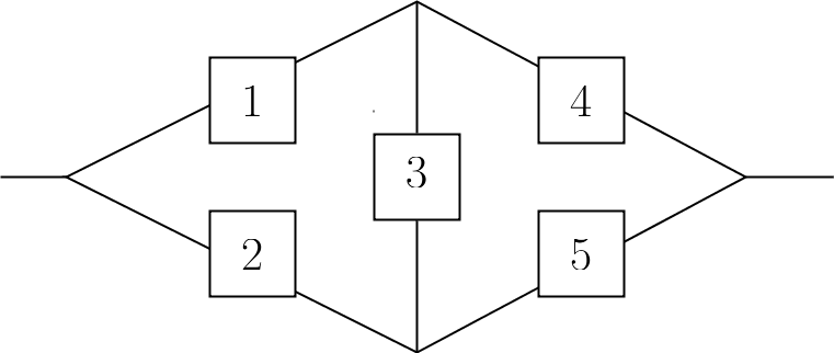
Figure 2: Block Diagram of a Bridge Structure

Figure 2 gives the logical block diagram for a system with a bridge-style reliability. Some communications networks may use a bridge system when there are alternative ways of connecting devices such as telephones or computers. The bridge system provides many possible ways to “complete the circuit” for relatively few components compared to a parallel system with higher reliability than a series system.

We still take each node to have its own arrival process; thus the diagram given above is logical and describes the various combinations of working components required for the system to work. It can be easily seen that the system survives past time $t$ if any one of the following sets of components all survive past $t$:

$$\{1,3,5\}\quad\{1,4\}\quad\{2,3,4\}\quad\{2,5\}$$

Thus we may give an equivalent block diagram of the bridge system using repeated components in Figure 3.

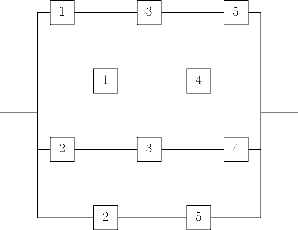
Figure 3: Alternative Representation of a Bridge Structure

Then the structure function may be easily derived using prior knowledge of series and parallel systems by breaking the above diagram into a parallel system of series subsystems. Therefore,

$$\phi(\mathbf{x})=1-(1-x_{1}x_{3}x_{5})(1-x_{1}x_{4})(1-x_{2}x_{3}x_{4})(1-x_{2}x_{5})$$

Expanding the above and replacing $x_{\ell}$ by $P(Y_{\ell}>t|N_{c}(t),\{\mathcal{H}_{j_{c}}\},\{T_{j_{c}}\},\{W_{j_{c}}\})$ one may derive the conditional survival function for the bridge system. Let $\mathcal{S}_{j_{c}}=\sum_{j_{c}=1}^{N_{c}(t)}\mathcal{H}_{j_{c}}\min(W_{j_{c}},t-T_{j_{c}})$, and let $f^{r,q}_{\mathcal{H}}(t)=q\mathcal{H}\int_{0}^{t}e^{-q\mathcal{H}w}m_{r}(t-w)\bar{G}_{w}(w)dw$, where $r=\{1,...,5,c\}$ and $q\in\mathbb{N}$. Then

$$P( Y_{S}>t|N_{c}(t),\{\mathcal{H}_{j_{c}}\},\{T_{j_{c}}\},\{W_{j_{c}}\})$$

$$=e^{-2\mathcal{S}_{j_{c}}}\left[\bar{F}_{0_{1}}(t)\bar{F}_{0_{4}}(t)\exp\left(-E_{\mathcal{H}}\left[f_{\mathcal{H}}^{1,1}(t)+f_{\mathcal{H}}^{4,1}(t)\right]\right)\right.$$

$$\hskip 72.26999pt+\left.\bar{F}_{0_{2}}(t)\bar{F}_{0_{5}}(t)\exp\left(-E_{\mathcal{H}}\left[f_{\mathcal{H}}^{2,1}(t)+f_{\mathcal{H}}^{5,1}(t)\right]\right)\right]$$

$$+e^{-3\mathcal{S}_{j_{c}}}\left[\bar{F}_{0_{1}}(t)\bar{F}_{0_{3}}(t)\bar{F}_{0_{5}}(t)\exp\left(-E_{\mathcal{H}}\left[f_{\mathcal{H}}^{1,1}(t)+f_{\mathcal{H}}^{3,1}(t)+f_{\mathcal{H}}^{5,1}(t)\right]\right)\right.$$

$$\hskip 72.26999pt+\left.\bar{F}_{0_{2}}(t)\bar{F}_{0_{3}}(t)\bar{F}_{0_{4}}(t)\exp\left(-E_{\mathcal{H}}\left[f_{\mathcal{H}}^{2,1}(t)+f_{\mathcal{H}}^{3,1}(t)+f_{\mathcal{H}}^{4,1}(t)\right]\right)\right]$$

$$-e^{-4\mathcal{S}_{j_{c}}}\left[\bar{F}_{0_{1}}(t)\bar{F}_{0_{2}}(t)\bar{F}_{0_{4}}(t)\bar{F}_{0_{5}}(t)\exp\left(-E_{\mathcal{H}}\left[f_{\mathcal{H}}^{1,1}(t)+f_{\mathcal{H}}^{2,1}(t)+f_{\mathcal{H}}^{4,1}(t)+f_{\mathcal{H}}^{5,1}(t)\right]\right)\right]$$

$$-e^{-5\mathcal{S}_{j_{c}}}\left[\bar{F}_{0_{1}}(t)\bar{F}_{0_{3}}(t)\bar{F}_{0_{5}}(t)\exp\left(-E_{\mathcal{H}}\left[f_{\mathcal{H}}^{1,1}(t)+f_{\mathcal{H}}^{3,1}(t)+f_{\mathcal{H}}^{5,1}(t)\right]\right)\right.$$

$$\hskip 72.26999pt+\bar{F}_{0_{1}}^{2}(t)\bar{F}_{0_{3}}(t)\bar{F}_{0_{4}}(t)\bar{F}_{0_{5}}(t)\exp\left(-E_{\mathcal{H}}\left[2f_{\mathcal{H}}^{1,1}(t)+f_{\mathcal{H}}^{3,1}(t)+f_{\mathcal{H}}^{4,1}(t)+f_{\mathcal{H}}^{5,1}(t)\right]\right)$$

$$\hskip 72.26999pt+\bar{F}_{0_{2}}^{2}(t)\bar{F}_{0_{3}}(t)\bar{F}_{0_{4}}(t)\bar{F}_{0_{5}}(t)\exp\left(-E_{\mathcal{H}}\left[2f_{\mathcal{H}}^{2,1}(t)+f_{\mathcal{H}}^{3,1}(t)+f_{\mathcal{H}}^{4,1}(t)+f_{\mathcal{H}}^{5,1}(t)\right]\right)$$

$$\hskip 72.26999pt+\bar{F}_{0_{4}}^{2}(t)\bar{F}_{0_{1}}(t)\bar{F}_{0_{2}}(t)\bar{F}_{0_{3}}(t)\exp\left(-E_{\mathcal{H}}\left[2f_{\mathcal{H}}^{4,1}(t)+f_{\mathcal{H}}^{1,1}(t)+f_{\mathcal{H}}^{2,1}(t)+f_{\mathcal{H}}^{3,1}(t)\right]\right)$$

$$\hskip 72.26999pt+\left.\bar{F}_{0_{5}}^{2}(t)\bar{F}_{0_{1}}(t)\bar{F}_{0_{2}}(t)\bar{F}_{0_{3}}(t)\exp\left(-E_{\mathcal{H}}\left[2f_{\mathcal{H}}^{5,1}(t)+f_{\mathcal{H}}^{1,1}(t)+f_{\mathcal{H}}^{2,1}(t)+f_{\mathcal{H}}^{3,1}(t)\right]\right)\right]$$

$$-e^{-6\mathcal{S}_{j_{c}}}\left[\bar{F}_{0_{1}}(t)\bar{F}_{0_{2}}(t)\bar{F}_{0_{3}}^{2}(t)\bar{F}_{0_{4}}(t)\bar{F}_{0_{5}}(t)\exp\left(-E_{\mathcal{H}}\left[2f_{\mathcal{H}}^{3,1}(t)+f_{\mathcal{H}}^{1,1}(t)+f_{\mathcal{H}}^{2,1}(t)+f_{\mathcal{H}}^{4,1}(t)+f_{\mathcal{H}}^{5,1}(t)\right]\right)\right]$$

$$+e^{-7\mathcal{S}_{j_{c}}}\left[\bar{F}_{0_{1}}^{2}(t)\bar{F}_{0_{2}}(t)\bar{F}_{0_{3}}(t)\bar{F}_{0_{4}}(t)\bar{F}^{2}_{0_{5}}(t)\exp\left(-E_{\mathcal{H}}\left[2f_{\mathcal{H}}^{1,1}(t)+f_{\mathcal{H}}^{2,1}(t)+f_{\mathcal{H}}^{3,1}(t)+f_{\mathcal{H}}^{4,1}(t)+2f_{\mathcal{H}}^{5,1}(t)\right]\right)\right.$$

$$\hskip 25.29494pt+\bar{F}_{0_{1}}(t)\bar{F}_{0_{2}}^{2}(t)\bar{F}_{0_{3}}(t)\bar{F}_{0_{4}}^{2}(t)\bar{F}_{0_{5}}(t)\exp\left(-E_{\mathcal{H}}\left[2f_{\mathcal{H}}^{2,1}(t)+f_{\mathcal{H}}^{1,1}(t)+f_{\mathcal{H}}^{3,1}(t)+2f_{\mathcal{H}}^{4,1}(t)+2f_{\mathcal{H}}^{5,1}(t)\right]\right)$$

$$\hskip 25.29494pt+\left.\bar{F}_{0_{1}}(t)\bar{F}_{0_{2}}^{2}(t)\bar{F}_{0_{3}}^{2}(t)\bar{F}_{0_{4}}(t)\bar{F}_{0_{5}}(t)\exp\left(-E_{\mathcal{H}}\left[2f_{\mathcal{H}}^{2,1}(t)+f_{\mathcal{H}}^{1,1}(t)+2f_{\mathcal{H}}^{3,1}(t)+f_{\mathcal{H}}^{4,1}(t)+2f_{\mathcal{H}}^{5,1}(t)\right]\right)\right]$$

$$+e^{-8\mathcal{S}_{j_{c}}}\left[\bar{F}_{0_{1}}^{2}(t)\bar{F}_{0_{2}}(t)\bar{F}_{0_{3}}^{2}(t)\bar{F}_{0_{4}}^{2}(t)\bar{F}_{0_{5}}(t)\exp\left(-E_{\mathcal{H}}\left[2f_{\mathcal{H}}^{1,1}(t)+f_{\mathcal{H}}^{2,1}(t)+2f_{\mathcal{H}}^{3,1}(t)+2f_{\mathcal{H}}^{4,1}(t)+f_{\mathcal{H}}^{5,1}(t)\right]\right)\right]$$

$$-e^{-9\mathcal{S}_{j_{c}}}\left[\bar{F}_{0_{1}}^{2}(t)\bar{F}_{0_{2}}^{2}(t)\bar{F}_{0_{3}}^{2}(t)\bar{F}_{0_{4}}^{2}(t)\bar{F}_{0_{5}}(t)\exp\left(-E_{\mathcal{H}}\left[2f_{\mathcal{H}}^{1,1}(t)+2f_{\mathcal{H}}^{2,1}(t)+2f_{\mathcal{H}}^{3,1}(t)+2f_{\mathcal{H}}^{4,1}(t)+f_{\mathcal{H}}^{5,1}(t)\right]\right)\right]$$

We may use the linearity of expectation to simply replace $e^{-q\mathcal{S}_{j_{c}}}$ by $\exp\left(E_{\mathcal{H}}\left[f_{\mathcal{H}}^{q,c}\right]\right)$ in  (LABEL:eq:_conditional_survival_function_bridge_system) to obtain $S_{Y_{S}}(t)$ for the bridge system. While not completely tractable, the survival function is given in closed form and illustrates a general technique wherein we may use the expansion of a structure function in order to derive the conditional survival function for any system where all components are correlated by one process $\{N_{c}(t)\}$. This conditional survival function will always be linear in $e^{-q\mathcal{S}_{j_{c}}}$, and thus the unconditional survival function may be easily obtained using the already well-developed method. We illustrate this with another example.

 4.2. $k$-of-$n$ System

The $k$-of-$n$ system has $n$ nodes in parallel of which $k$ must be functioning in order for the system to remain functioning. This is a generalization of the series system ($n$-of-$n$) and the parallel system ($1$-of-$n$). The structure function of a $k$-of-$n$ system is given by

$$\phi(\mathbf{x})=1-\prod\limits_{\tiny\begin{subarray}{c}\ell_{j}=1;\\ j=1,...,k\\ \ell_{1}<...<\ell_{k}\end{subarray}}^{n}\left(1-\prod_{j=1}^{k}x_{\ell_{j}}\right)$$ (15)

By replacing $\ell_{j}$ with the appropriate conditional survival function for component $\ell$ and expanding (15), we may again arrive at the system survival function conditioned upon $\{N_{c}(t):t\geq 0\}$. Because this system may also be expressed as a parallel system of series subsystems, the conditional survival function will again be linear in $e^{-q\mathcal{S}_{j_{c}}}$ and thus the linearity of expectation allows for straightfoward computation of the system survival function.

4.2.1 Example: 2-of-3 system

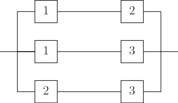
Figure 4: Block Diagram of 2-of-3 System

Figure 4 gives the logical block diagram for a 2-of-3 system. Thus, using  (15), the structure function for the 2-of-3 system is given by

$$\phi(\mathbf{x}) =1-(1-x_{1}x_{2})(1-x_{1}x_{3})(1-x_{2}x_{3})$$

$$=\sum_{i=1}^{2}\sum_{j=i+1}^{3}x_{i}x_{j}-\sum\limits_{\begin{subarray}{c}i=1\\ j,k\neq i\end{subarray}}^{3}x_{i}^{2}x_{j}x_{k}+\prod_{i=1}^{3}x_{i}^{2}$$ (16)

Using the technique described in Section 4.1, one may arrive at the unconditional survival function of the 2-of-3 system:

$$S_{Y_{S}}(t) =\exp\left(-E_{\mathcal{H}}[f_{\mathcal{H}}^{c,2}(t)]\right)\left[\sum_{i=1}^{2}\sum_{j=i+1}^{3}\bar{F}_{0_{i}}(t)\bar{F}_{0_{j}}(t)\exp\left(-E_{\mathcal{H}}[f_{\mathcal{H}}^{i,1}(t)+f_{\mathcal{H}}^{j,1}(t)]\right)\right]$$

$$\quad\exp\left(-E_{\mathcal{H}}[f_{\mathcal{H}}^{c,4}(t)]\right)\left[\sum\limits_{\begin{subarray}{c}i=1\\ j,k\neq i\end{subarray}}^{3}\bar{F}_{0_{i}}^{2}(t)\bar{F}_{0_{j}}(t)\bar{F}_{0_{k}}(t)\exp\left(-E_{\mathcal{H}}\left[2f_{\mathcal{H}}^{i,1}(t)+f_{\mathcal{H}}^{j,1}(t)+f_{\mathcal{H}}^{k,1}(t)\right]\right)\right]$$

$$\quad+\exp\left(-E_{\mathcal{H}}[f_{\mathcal{H}}^{c,6}(t)]\right)\left(\prod_{\ell=1}^{3}\bar{F}_{0_{\ell}}^{2}(t)\right)\exp\left(-E_{\mathcal{H}}\left[2\sum_{\ell=1}^{3}f_{\mathcal{H}}^{\ell,1}(t)\right]\right)$$ (17)

 5. CONCLUSION

In [3], Traylor derived the survival function for a single server under workload where the arrivals may be described by a NHPP and the workload stresses are random. We created a logical system of such servers correlated by a nonhomogenous “correlator” Poisson process; thus each node is conditionally independent. The conditional survival function for each server (or node) is found to be in one-to-one correspondence with the binary state (operational or failed) $x_{\ell}$, and thus the system structure function is isomorphic to the system’s conditional survival function. This gives a straightforward method to compute the conditional survival function of the correlated system. All structure functions may be derived using series and parallel structure functions, and both series and parallel structure functions are linear in $e^{-q\mathcal{S}_{j_{c}}}$, where $\mathcal{S}_{j_{c}}=\sum_{j_{c}=1}^{N_{c}(t)}\mathcal{H}_{j_{c}}\min(W_{j_{c}},t-T_{j_{c}})$. The unconditional survival function is calculated by taking the expectation over $N_{c}(t)$, and thus the linearity of expectation allows for a straightfoward computation of the system survival function.

This method allows for the modeling of more complex logical system architectures without simplification of the arrival process or the assumption of node independence.

Appendix A APPENDIX

Lemma A.1.

Let $\{N_{i}(t):t\geq 0\}_{i=1}^{n}$ be independent nonhomogeneous Poisson processes with intensities $\lambda_{i}(t),i=1,...,n$. Let $N(t)=\sum_{i=1}^{n}N_{i}(t)$ is a nonhomogeneous Poisson process with intensity $\lambda(t)=\sum_{i=1}^{n}\lambda_{i}(t)$

Proof.

The proof will proceed via induction. As a base case, let $n=2$. It suffices to show that $N(0)=0$, and

$$P(N(t+s)-N(t)=n)=\dfrac{\exp\left(-(m(t+s)-m(t))\right)[m(t+s)-m(t)]^{n}}{n!}$$

where $m(t)=m_{1}(t)+m_{2}(t)$ and $m_{i}(t)=\int_{0}^{t}\lambda_{i}(s)ds$. Clearly, $N(0)=N_{1}(0)+N_{2}(0)=0+0=0$. Now, since $\{N_{1}(t)\},\{N_{2}(t)\}$ are independent, we may find the distribution of $\{N(t)\}$ via convolution. Thus,

$$P(N(t+s) -N(t)=n)$$

$$=P((N_{1}+N_{2})(t+s)-(N_{1}+N_{2})(t))=n)$$

$$=P(N_{1}(t+s)+N_{2}(t+s)-N_{1}(t)-N_{2}(t)=n)$$

$$=\sum_{x=0}^{n}P([N_{1}(t+s)-N_{1}(t)=x]\cap[N_{2}(t+s)-N_{2}(t)=n-x])$$

$$=\sum_{x=0}^{n}P(N_{1}(t+s)-N_{1}(t)=x)P(N_{2}(t+s)-N_{2}(t)=n-x)$$

$$=\sum_{x=0}^{n}\frac{(m_{1}(t+s)-m_{1}(t))^{x}e^{-(m_{1}(t+s)-m_{1}(t))}}{x!}\frac{(m_{2}(t-s)-m_{2}(t))^{n-x}e^{-(m_{2}(t+s)-m_{2}(t))}}{(n-x)!}$$

$$=\frac{1}{n!}e^{-(m_{1}+m_{2})(t+s)-(m_{1}+m_{2})(t)}\sum_{x=0}^{n}\frac{n!}{x!(n-x)!}(m_{1}(t+s)-m_{1}(t))^{x}(m_{2}(t+s)-m_{2}(t))^{n-x}$$

$$=\frac{1}{n!}e^{-(m_{1}+m_{2})(t+s)-(m_{1}+m_{2})(t)}(m_{1}(t+s)-m_{1}(t)+m_{2}(t+s)-m_{2}(t))^{n}$$

$$=\frac{e^{-(m_{1}+m_{2})(t+s)-(m_{1}+m_{2})(t)}}{n!}((m_{1}+m_{2})(t+s)-(m_{1}+m_{2})(t))^{n}$$

$$=\frac{e^{-(\lambda_{1}+\lambda_{2})(s)}(\lambda_{1}+\lambda_{2})(s))^{n}}{n!}$$

Now, assume that $N_{\kappa}(t)=\sum_{i=1}^{k}N_{i}(t)$ is a NHPP with intensity $\lambda(t)=\sum_{i=1}^{k}\lambda_{i}(t)$. Then let $N(t)=N_{\kappa}(t)+N_{k+1}(t)$, where $\{N_{k+1}(t)\}$ is a NHPP with intensity $\lambda_{k+1}(t)$. Then using the same procedure as above, we see that

$$P(N(t+s)-N(t)=n)=\frac{e^{-\left(\sum_{i=1}^{k+1}\lambda_{i}\right)(s)}(\left(\sum_{i=1}^{k+1}\lambda_{i}\right)(s))^{n}}{n!}$$

and thus the sum of nonhomogeneous Poisson processes remains a NHPP. ∎

Lemma A.2.

Under the condition that $N_{c}(t)=n_{c},\mathcal{H}_{j_{c}}=\eta_{i_{j_{c}}},i\in\{1,...,m\},j_{c}=1,...,n_{c}$, we have that

$$P\left(\right.Y_{\ell,c}>t \left|N_{c}(t),\{T_{j_{c}}\}_{j_{c}=1}^{N_{c}(t)},\{W_{j_{c}}\}_{j_{c}=1}^{N_{c}(t)},\{\mathcal{H}_{j_{c}}\}_{j_{c}=1}^{N_{c}(t)}\right.\left.\right)$$

$$=\bar{F}_{0_{\ell,c}}\exp\left(-\sum_{j_{c}=1}^{N_{c}(t)}\mathcal{H}_{j_{c}}\min(W_{j_{c}},t-T_{j_{c}})\right)\exp\left(-E_{\mathcal{H}}\left[\mathcal{H}\int_{0}^{t}\exp(-\mathcal{H}w)m_{\ell}(t-w)\bar{G}_{W}(w)dw\right]\right)$$

where $m_{\ell}(x)=\int_{0}^{x}\lambda_{\ell}(s)ds$.

Proof.

As before ([3]), we have that

$$P\left(\right.Y_{\ell}>t \left|N_{c}(t),\{T_{j_{c}}\}_{j_{c}=1}^{N_{c}(t)},\{W_{j_{c}}\}_{j_{c}=1}^{N_{c}(t)},\{\mathcal{H}_{j_{c}}\}_{j_{c}=1}^{N_{c}(t)},N_{\ell}(t),\{T_{j_{\ell}}\}_{j_{\ell}=1}^{N_{\ell}(t)},\{W_{j_{\ell}}\}_{j_{\ell}=1}^{N_{\ell}(t)},\{\mathcal{H}_{j_{\ell}}\}_{j_{\ell}=1}^{N_{\ell}(t)}\right.\left.\right)$$

$$=\exp\left(-\int_{0}^{t}\mathcal{B}_{\ell}(t)\right)$$

$$=\bar{F}_{0_{1}}(t)\exp\left(-\sum_{j_{\ell}=1}^{N_{\ell}(t)}\mathcal{H}_{j_{\ell}}\min(W_{j_{\ell}},t-T_{j_{\ell}})-\sum_{j_{c}=1}^{N_{c}(t)}\mathcal{H}_{j_{c}}\min(W_{j_{c}},t-T_{j_{c}})\right)$$

$$=\bar{F}_{0_{1}}(t)\exp\left(-\sum_{j_{\ell}=1}^{N_{\ell}(t)}\mathcal{H}_{j_{\ell}}\min(W_{j_{\ell}},t-T_{j_{\ell}})\right)\exp\left(-\sum_{j_{c}=1}^{N_{c}(t)}\mathcal{H}_{j_{c}}\min(W_{j_{c}},t-T_{j_{c}})\right)$$ (19)

Now,

$$P\left(\right.Y_{\ell,c}>t \left|N_{c}(t),\{T_{j_{c}}\}_{j_{c}=1}^{N_{c}(t)},\{W_{j_{c}}\}_{j_{c}=1}^{N_{c}(t)},\{\mathcal{H}_{j_{c}}\}_{j_{c}=1}^{N_{c}(t)}\right.\left.\right)$$

$$=E_{N_{\ell},\{\mathcal{H}_{j_{\ell}}\}}\left[\bar{F}_{0_{\ell,c}}(t)\exp\left(-\sum_{j_{\ell}=1}^{N_{\ell}(t)}\mathcal{H}_{j_{\ell}}\min(W_{j_{\ell}},t-T_{j_{\ell}})\right)\exp\left(-\sum_{j_{c}=1}^{N_{c}(t)}\mathcal{H}_{j_{c}}\min(W_{j_{c}},t-T_{j_{c}})\right)\right]$$

$$=\bar{F}_{0_{\ell,c}}\exp\left(-\sum_{j_{c}=1}^{N_{c}(t)}\mathcal{H}_{j_{c}}\min(W_{j_{c}},t-T_{j_{c}})\right)E_{N_{\ell},\{\mathcal{H}_{j_{\ell}}\}}\left[\exp\left(-\sum_{j_{\ell}=1}^{N_{\ell}(t)}\mathcal{H}_{j_{\ell}}\min(W_{j_{\ell}},t-T_{j_{\ell}})\right)\right]$$

But this case reduces to the previous RSBR case, and hence we have

$$=\bar{F}_{0_{\ell,c}}\exp\left(-\sum_{j_{c}=1}^{N_{c}(t)}\mathcal{H}_{j_{c}}\min(W_{j_{c}},t-T_{j_{c}})\right)\exp\left(-E_{\mathcal{H}}\left[\mathcal{H}\int_{0}^{t}\exp(-\mathcal{H}w)m(t-w)\bar{G}_{W}(w)dw\right]\right)$$

∎

References

• [1] Cha, K. H., and Lee, E. Y. A stochastic breakdown model for an unreliable web server system and an optimal admission control policy. Journal of Applied Probability 48, 2 (2011), 453–466.
• [2] Leemis, L. M. Reliability: Probabilistic Models and Statistical Methods, 2nd edition. Prentice-Hall, 2009.
• [3] Traylor, R. A stochastic reliability model of a server under a random workload. preprint arXiv:1511.04130 (2015).