Strong-stability-preserving additive linear multistep methods

Abstract

The analysis of strong-stability-preserving (SSP) linear multistep methods is extended to semi-discretized problems for which different terms on the right-hand side satisfy different forward Euler (or circle) conditions. Optimal additive and perturbed monotonicity-preserving linear multistep methods are studied in the context of such problems. Optimal perturbed methods attain larger monotonicity-preserving step sizes when the different forward Euler conditions are taken into account. On the other hand, we show that optimal SSP additive methods achieve a monotonicity-preserving step-size restriction no better than that of the corresponding non-additive SSP linear multistep methods.

1 Introduction

We are interested in numerical solutions of initial value ODEs

$$\begin{split}\bm{u}^{\prime}(t)&=\bm{F}(\bm{u}(t)),\quad t\geq t_{0}\\ \bm{u}(t_{0})&=\bm{u}_{0},\end{split}$$ (1.1)

where $\bm{F}:\mathbb{R}^{m}\rightarrow\mathbb{R}^{m}$ is a continuous function and $\bm{u}:[t_{0},\infty)\rightarrow\mathbb{R}^{m}$ satisfies a monotonicity property

$$\|\bm{u}(t+\Delta t)\|\leq\|\bm{u}(t)\|,\quad\forall\Delta t\geq 0,$$ (1.2)

with respect to some norm, semi-norm or convex functional $\|\cdot\|:\mathbb{R}^{m}\rightarrow\mathbb{R}$. In general $\bm{F}(\bm{u}(t))$ may arise from the spatial discretization of partial differential equations; for example, hyperbolic conservation laws. A sufficient condition for monotonicity is that there exists some $\Delta t_{\textnormal{FE}}>0$ such that the forward Euler condition

$$\|\bm{u}+\Delta t\bm{F}(\bm{u})\|\leq\|\bm{u}\|,\quad 0\leq\Delta t\leq\Delta t_{\textnormal{FE}},$$ (1.3)

holds for all $\bm{u}\in\mathbb{R}^{m}$.

In this paper we focus on linear multistep method s (LMMs) for the numerical integration of (1.1). We denote by $\bm{u}_{n}$ the numerical approximation to $\bm{u}(t_{n})$, evaluated sequentially at times $t_{n}=t_{0}+n\Delta t$, $n\geq 1$. At step $n$, a $k$-step linear multistep method applied to (1.1) takes the form

$$\bm{u}_{n}=\sum_{j=0}^{k-1}\alpha_{j}\bm{u}_{n-k+j}+\Delta t\sum_{j=0}^{k}\beta_{j}\bm{F}(\bm{u}_{n-k+j})$$ (1.4)

and if $\beta_{k}=0$, then the method is explicit.

We would like to establish a discrete analogue of (1.2) for the numerical solution $\bm{u}_{n}$ in (1.4). Assuming $\bm{F}$ satisfies the forward Euler condition (1.3) and all $\alpha_{j},\beta_{j}$ are non-negative, then convexity of $\|\cdot\|$ and the consistency requirement $\sum_{j=0}^{k-1}\alpha_{j}=1$ imply that $\|\bm{u}_{n}\|\leq\max_{j}\|\bm{u}_{n-k+j}\|$ whenever $\Delta t\beta_{j}/\alpha_{j}\leq\Delta t_{\textnormal{FE}}$ for all $j$. Hence, the monotonicity condition

$$\|\bm{u}_{n}\|\leq\max\{\|\bm{u}_{n-1}\|,\dots,\|\bm{u}_{n-k}\|\}.$$ (1.5)

is satisfied under a step-size restriction

$$\Delta t\leq\mathcal{C}_{\text{LMM}}\Delta t_{\textnormal{FE}},$$ (1.6)

where $\mathcal{C}_{\text{LMM}}=\min_{j}\alpha_{j}/\beta_{j}$. The ratio $\alpha_{j}/\beta_{j}$ is taken to be infinity if $\beta_{j}=0$. See [3, Chapter 8] and references therein for a review of strong-stability-preserving linear multistep method s (SSP LMMs).

Most LMMs have one or more negative coefficients, so the foregoing analysis leads to $\mathcal{C}_{\text{LMM}}=0$ and thus monotonicity condition (1.5) cannot be guaranteed by positive step sizes. However, typical numerical methods for hyperbolic conservation laws $\bm{U}_{t}+\nabla\!\cdot\!\bm{f}(\bm{U})=0$ involve upwind-biased semi-discretizations of the spatial derivatives. In order to preserve monotonicity using methods with negative coefficients for such semi-discretizations, downwind-biased spatial approximations may be used. Let $\bm{F}$ and $\widetilde{\bm{F}}$ be respectively upwind- and downwind-biased approximations of $-\nabla\!\cdot\!\bm{f}(\bm{U})$. It is natural to assume that $\widetilde{\bm{F}}$ satisfies

$$\|\bm{u}-\Delta t\bm{F}(\bm{u})\|\leq\|\bm{u}\|,\quad 0\leq\Delta t\leq\Delta t_{\textnormal{FE}},$$ (1.7)

for all $\bm{u}\in\mathbb{R}^{m}$. A linear multistep method that uses both $\bm{F}$ and $\widetilde{\bm{F}}$ can be then written as

$$\bm{u}_{n}=\sum_{j=0}^{k-1}\alpha_{j}\bm{u}_{n-k+j}+\Delta t\sum_{j=0}^{k}\left(\beta_{j}\bm{F}(\bm{u}_{n-k+j})-\tilde{\beta}_{j}\widetilde{\bm{F}}(\bm{u}_{n-k+j})\right).$$ (1.8)

If all $\alpha_{j}$ are non-negative, then the method is monotonicity preserving under the restriction (1.6) where the SSP coefficient is now $\widetilde{\mathcal{C}}_{\text{LMM}}=\min_{j}\alpha_{j}/(\beta_{j}+\tilde{\beta}_{j})$ with $\beta_{j}$, $\tilde{\beta}_{j}$ non-negative; see [3, Chapter 10] and the references therein.

Downwind LMMs were originally introduced in [17, 18], with the idea that $\bm{F}$ be replaced by $\widetilde{\bm{F}}$ whenever $\beta_{j}<0$. Optimal explicit linear multistep schemes of order up to six, coupled with efficient upwind and downwind WENO discretizations, were studied in [4]. Coefficients of optimal upwind- and downwind-biased methods together with a reformulation of the nonlinear optimization problem involved as a series of linear programming feasibility problems can be found in [10]. Bounds on the maximum SSP step size for downwind-biased methods have been analyzed in [11].

Method (1.8) can also be written in the perturbed form

$$\bm{u}_{n}=\sum_{j=0}^{k-1}\alpha_{j}\bm{u}_{n-k+j}+\Delta t\sum_{j=0}^{k}\left(\invbreve{\beta}_{j}\bm{F}(\bm{u}_{n-k+j})+\tilde{\beta}_{j}\left(\bm{F}(\bm{u}_{n-k+j})-\widetilde{\bm{F}}(\bm{u}_{n-k+j})\right)\right),$$ (1.9)

where $\invbreve{\beta}_{j}=\beta_{j}-\tilde{\beta}_{j}$. We say method (1.9) is a perturbation of the LMM (1.4) with coefficients $\invbreve{\beta}_{j}$, and the latter is referred to as the underlying method for (1.9). By replacing $\widetilde{\bm{F}}$ with $\bm{F}$ in (1.9) one recovers the underlying method. The notion of a perturbed method can be useful beyond the realm of downwinding for hyperbolic PDE semi-discretizations. If $\bm{F}$ satisfies the forward Euler condition (1.3) for both positive and negative step sizes, then we can simply take $\widetilde{\bm{F}}=\bm{F}$. In such cases, the perturbed and underlying methods are the same, but analysis of a perturbed form of the method can yield a larger step size for monotonicity, giving more accurate insight into the behavior of the method. See [7] for a discussion of this in the context of Runge–Kutta methods, and see Example 2.2 herein for an example using multistep methods. As we will see in Section 2, the most useful perturbed LMM s (1.9) take a form in which either $\beta_{j}$ or $\tilde{\beta}_{j}$ is equal to zero for each value of $j$. Thus $\widetilde{\mathcal{C}}_{\text{LMM}}=\min_{j}\{\alpha_{j}/\beta_{j},\alpha_{j}/\tilde{\beta}_{j}\}$, and the class of perturbed LMM s (1.9) coincides with the class of downwind LMMs in [17, 18].

In this work, we adopt form (1.8) for perturbed LMM s and consider their application to the more general class of problems (1.1) for which $\bm{F}$ and $\widetilde{\bm{F}}$ satisfy forward Euler conditions under different step-size restrictions:

$$\|\bm{u}+\Delta t\bm{F}(\bm{u})\|\leq\|\bm{u}\|, \quad\forall\bm{u}\in\mathbb{R}^{m},\;0\leq\Delta t\leq\Delta t_{\textnormal{FE}}$$ (1.10a)

$$\|\bm{u}-\Delta t\widetilde{\bm{F}}(\bm{u})\|\leq\|\bm{u}\|, \quad\forall\bm{u}\in\mathbb{R}^{m},\;0\leq\Delta t\leq\widetilde{\Delta t}_{\textnormal{FE}}.$$ (1.10b)

For a fixed order of accuracy and number of steps, an optimal SSP method is defined to be any method that attains the largest possible SSP coefficient. The choice of optimal monotonicity-preserving method for a given problem will depend on the ratio $y=\Delta t_{\textnormal{FE}}/\widetilde{\Delta t}_{\textnormal{FE}}$. We analyze and construct such optimal methods. We illustrate by examples that perturbed LMM s with larger step sizes for monotonicity can be obtained when the different step sizes in (1.10) are accounted for.

The perturbed methods (1.8) are reminiscent of additive methods, and the latter can be analyzed in a similar way. Consider the problem

$$\bm{u}^{\prime}(t)=\bm{F}(\bm{u}(t))+\widehat{\bm{F}}(\bm{u}(t))$$

where $\bm{F}$ and $\widehat{\bm{F}}$ may represent different physical processes, such as convection and diffusion or convection and reaction. Additive methods are expressed as

$$\bm{u}_{n}=\sum_{j=0}^{k-1}\alpha_{j}\bm{u}_{n-k+j}+\Delta t\sum_{j=0}^{k}\left(\beta_{j}\bm{F}(\bm{u}_{n-k+j})+\hat{\beta}_{j}\widehat{\bm{F}}(\bm{u}_{n-k+j})\right),$$

where $\bm{F}$ and $\widehat{\bm{F}}$ may satisfy the forward Euler condition (1.3) under possibly different step-size restrictions. We prove that optimal SSP explicit or implicit additive methods have coefficients $\beta_{j}=\hat{\beta}_{j}$ for all $j$, hence they lie within the class of ordinary (not additive) LMMs.

The rest of the paper is organized as follows. In Section 2 we analyze the monotonicity properties of perturbed LMM s for which the upwind and downwind operators satisfy different forward Euler conditions. Optimal methods are derived, and their properties are discussed. Their effectiveness is illustrated by some examples. Additive linear multistep method s are presented in Section 3 where we prove that optimal SSP additive LMM s are equivalent to the corresponding non-additive SSP LMMs. Monotonicity of IMEX linear multistep method s is discussed, and finally in Section 4 we summarize the main results.

2 Monotonicity-preserving perturbed linear multistep method s

The following example shows that using upwind- and downwind-biased operators allows the construction of methods that have positive SSP coefficients, even though the underlying methods are not SSP.

Example 2.1.

Let $u^{\prime}(t)=F(u(t))$ be a semi-discretization of $u_{t}+f(u)_{x}=0$, where $F\approx-f(u)_{x}$. Consider the two-step, second-order explicit linear multistep method

$$u_{n}=\frac{1}{2}u_{n-2}-\frac{1}{4}\Delta tF(u_{n-2})+\frac{1}{2}u_{n-1}+\frac{7}{4}\Delta tF(u_{n-1}).$$ (2.1)

The method has SSP coefficient equal to zero. Let us introduce a downwind-biased operator $\widetilde{F}\approx-f(u)_{x}$ such that (1.7) is satisfied. Then, a perturbed representation of (2.1) is

$$u_{n}=\frac{1}{2}u_{n-2}+\frac{1}{4}\Delta tF(u_{n-2})-\frac{1}{2}\Delta t\widetilde{F}(u_{n-2})+\frac{1}{2}u_{n-1}+2\Delta tF(u_{n-1})-\frac{1}{4}\Delta t\widetilde{F}(u_{n-1}),$$ (2.2)

in the sense that the underlying method (2.1) is retrieved from (2.2) by replacing $\widetilde{F}$ with $F$. The perturbed method has SSP coefficient $\widetilde{\mathcal{C}}_{\text{LMM}}=2/9$. There are infinitely many perturbed representations of (2.1), but an optimal one is obtained by simply replacing $F$ with $\widetilde{F}$ in (2.1), yielding

$$u_{n}=\frac{1}{2}u_{n-2}-\frac{1}{4}\Delta t\widetilde{F}(u_{n-2})+\frac{1}{2}u_{n-1}+\frac{7}{4}\Delta tF(u_{n-1}),$$ (2.3)

with SSP coefficient $\widetilde{\mathcal{C}}_{\text{LMM}}=2/7$.

Remark 2.1.

A LMM (1.4) has SSP coefficient $\mathcal{C}=0$ if any of the following three conditions hold:

1. $\alpha_{j}<0$ for some $j$;

2. $\beta_{j}<0$ for some $j$;

3. $\alpha_{j}=0$ for some $j$ for which $\beta_{j}\neq 0$.

By introducing a downwind operator we can remedy the second condition, but not the first or the third. Most common methods, including the Adams–Bashforth, Adams–Moulton, and BDF methods, satisfy condition 1 or 3, so they cannot be made SSP via downwinding.

We consider a generalization of the perturbed LMM s described previously, by assuming different forward Euler conditions for the operators $\bm{F}$ and $\widetilde{\bm{F}}$ (see (1.10)).

Definition 2.1.

A perturbed LMM of the form (1.8) is said to be strong-stability-preserving (SSP) with SSP coefficients $(\mathcal{C},\widetilde{\mathcal{C}})$ if conditions

$$\begin{split}\beta_{j},\tilde{\beta}_{j}\geq 0,&\quad j\in\{0,\dots,k\},\\ \alpha_{j}-r\beta_{j}-\tilde{r}\tilde{\beta}_{j}\geq 0,&\quad j\in\{0,\dots,k-1\},\end{split}$$ (2.4)

hold for all $0\leq r\leq\mathcal{C}$ and $0\leq\tilde{r}\leq\widetilde{\mathcal{C}}$.

By plugging the exact solution in (1.8), setting $\widetilde{\bm{F}}(\bm{u}(t_{n}))=\bm{F}(\bm{u}(t_{n}))$ and taking Taylor expansions around $t_{n-k}$, it can be shown that a perturbed LMM is order $p$ accurate if

$$\begin{gathered}\sum_{j=0}^{k-1}\alpha_{j}=1,\qquad\sum_{j=0}^{k-1}j\alpha_{j}+\sum_{j=0}^{k}(\beta_{j}-\tilde{\beta}_{j})=k,\\ \sum_{j=0}^{k-1}\alpha_{j}j^{i}+\sum_{j=0}^{k}(\beta_{j}-\tilde{\beta}_{j})ij^{i-1}=k^{i},\quad i\in\{2,\dots,p\}.\end{gathered}$$ (2.7)

The step-size restriction for monotonicity of an SSP perturbed LMM is given by the following theorem.

Theorem 2.1.

Consider an initial value problem for which $\bm{F}$ and $\widetilde{\bm{F}}$ satisfy the forward Euler conditions (1.10) for some $\Delta t_{\textnormal{FE}}>0$, $\widetilde{\Delta t}_{\textnormal{FE}}>0$. Let a consistent perturbed LMM (1.8) be SSP with SSP coefficients $(\mathcal{C},\widetilde{\mathcal{C}})$. Then the numerical solution satisfies the monotonicity condition (1.5) under a step-size restriction

$$\Delta t\leq\min\{\mathcal{C}\,\Delta t_{\textnormal{FE}},\widetilde{\mathcal{C}}\,\widetilde{\Delta t}_{\textnormal{FE}}\}.$$ (2.8)

Proof.

Define $\alpha_{k}=\mathcal{C}\beta_{k}+\widetilde{\mathcal{C}}\tilde{\beta_{k}}$ and add $\alpha_{k}\bm{u}_{n}$ to both sides of (1.8) to obtain

$$(1+\alpha_{k})\bm{u}_{n}=\sum_{j=0}^{k}\left(\alpha_{j}\bm{u}_{n-k+j}-\Delta t\beta_{j}\bm{F}(\bm{u}_{n-k+j})+\Delta t\tilde{\beta}_{j}\widetilde{\bm{F}}(\bm{u}_{n-k+j})\right).$$

Since the method is SSP with coefficients $(\mathcal{C},\widetilde{\mathcal{C}})$ then conditions (2.4) hold for $r=\mathcal{C}$, $\tilde{r}=\widetilde{\mathcal{C}}$. Let $\alpha_{j}=\hat{\alpha}_{j}+\tilde{\alpha}_{j}$ with $\hat{\alpha}_{j}=\mathcal{C}\beta_{j}$. Then (2.4) yields $\tilde{\alpha}_{j}\geq\widetilde{\mathcal{C}}\tilde{\beta}_{j}$ and $\beta_{j}\geq 0,\tilde{\beta}_{j}\geq 0$. Thus, the right-hand side can be expressed as a convex combination of forward Euler steps:

$$(1+\alpha_{k})\bm{u}_{n}=\sum_{j=0}^{k}\hat{\alpha}_{j}\Bigl{(}\bm{u}_{n-k+j}+\Delta t\frac{\beta_{j}}{\hat{\alpha}_{j}}\bm{F}(\bm{u}_{n-k+j})\Bigr{)}+\sum_{j=0}^{k}\tilde{\alpha}_{j}\Bigl{(}\bm{u}_{n-k+j}-\Delta t\frac{\tilde{\beta}_{j}}{\tilde{\alpha}_{j}}\widetilde{\bm{F}}(\bm{u}_{n-k+j})\Bigr{)}.$$

Taking norms and using the triangle inequality yields

$$(1+\alpha_{k})\|\bm{u}_{n}\|\leq\sum_{j=0}^{k}\hat{\alpha}_{j}\Bigl{\|}\bm{u}_{n-k+j}+\Delta t\frac{\beta_{j}}{\hat{\alpha}_{j}}\bm{F}(\bm{u}_{n-k+j})\Bigr{\|}+\sum_{j=0}^{k}\tilde{\alpha}_{j}\Bigl{\|}\bm{u}_{n-k+j}-\Delta t\frac{\tilde{\beta}_{j}}{\tilde{\alpha}_{j}}\widetilde{\bm{F}}(\bm{u}_{n-k+j})\Bigr{\|}.$$

Under the step-size restriction $\Delta t\leq\min\{\mathcal{C}\,\Delta t_{\textnormal{FE}},\widetilde{\mathcal{C}}\,\widetilde{\Delta t}_{\textnormal{FE}}\}$ we get

$$\Delta t\frac{\beta_{j}}{\hat{\alpha}_{j}}\leq\Delta t_{\textnormal{FE}}\quad\text{and}\quad\Delta t\frac{\tilde{\beta}_{j}}{\tilde{\alpha}_{j}}\leq\widetilde{\Delta t}_{\textnormal{FE}}.$$

Since $\bm{F}$ and $\widetilde{\bm{F}}$ satisfy (1.10a) and (1.10b) respectively, we have

$$(1+\alpha_{k})\|\bm{u}_{n}\| \leq\sum_{j=0}^{k}\hat{\alpha}_{j}\|\bm{u}_{n-k+j}\|+\sum_{j=0}^{k}\tilde{\alpha}_{j}\|\bm{u}_{n-k+j}\|,$$

and hence

$$\|\bm{u}_{n}\|\leq\sum_{j=0}^{k-1}\alpha_{j}\|\bm{u}_{n-k+j}\|\leq\max_{0\leq j\leq k-1}\|\bm{u}_{n-k+j}\|\sum_{j=0}^{k-1}\alpha_{j}.$$

Consistency requires $\sum_{j=0}^{k-1}\alpha_{j}=1$ and therefore the monotonicity condition (1.5) follows. ∎

2.1 Optimal SSP perturbed linear multistep method s

We now turn to the problem of finding, among methods with a given number of steps $k$ and order of accuracy $p$, the largest SSP coefficients. Since $\mathcal{C}$, $\widetilde{\mathcal{C}}$ are continuous functions of the method’s coefficients, we expect that the maximal step size (2.8) is achieved when $\mathcal{C}=\widetilde{\mathcal{C}}\,\widetilde{\Delta t}_{\textnormal{FE}}/\Delta t_{\textnormal{FE}}$. It is thus convenient to define $y:=\Delta t_{\textnormal{FE}}/\widetilde{\Delta t}_{\textnormal{FE}}$.

Definition 2.2.

For a fixed $y\in[0,\infty)$ we say that an SSP method (1.8) has SSP coefficient

$$\mathcal{C}(y)=\sup\bigl{\{}r\geq 0:\text{monotonicity conditions \eqref{eq:DLMMMonCondDiffFE} hold with }\tilde{r}=yr\bigr{\}}$$

and its corresponding downwind SSP coefficient is $\widetilde{\mathcal{C}}(y)=y\,\mathcal{C}(y)$. Given a number of steps $k$ and order of accuracy $p$ an SSP method is called optimal, if it has SSP coefficient

$$\mathcal{C}_{k,p}(y)=\sup_{\bm{\alpha},\bm{\beta},\bm{\tilde{\beta}}}\bigl{\{}\mathcal{C}(y)>0:\mathcal{C}(y)\text{ is the SSP coefficient of a $k$-step method \eqref{eq:DLMM} of order $p$}\bigr{\}}.$$

Next we prove that for a given SSP perturbed LMM with SSP coefficient $\mathcal{C}(y)$, we can construct another SSP method (1.8) with the property that for each $j$, either $\beta_{j}$ or $\tilde{\beta}_{j}$ is zero. Example 2.1 is an application of this result.

Lemma 2.1.

Consider a $k$-step perturbed LMM (1.8) of order $p$ with SSP coefficient $\mathcal{C}(y)$ for a given $y$. Then, we can construct a $k$-step SSP method (1.8) of order $p$ with SSP coefficient at least $\mathcal{C}(y)$ that satisfies $\beta_{j}\tilde{\beta}_{j}=0$ for each $j$. Moreover, both perturbed methods correspond to the same underlying method.

Proof.

Suppose there exists an $k$-step SSP method (1.8) of order $p$ with SSP coefficient $\mathcal{C}(y)$ for some $y\in[0,\infty)$, such that $\beta_{j}\geq\tilde{\beta}_{j}>0$ for $j\in J_{1}\subseteq\{0,1,\dots,k\}$ and $\tilde{\beta}_{j}>\beta_{j}>0$ for $j\in J_{2}\subseteq\{0,1,\dots,k\}$. Clearly $J_{1}\cap J_{2}=\emptyset$. Define

$$\beta_{j}^{*}=\begin{cases}\beta_{j}-\tilde{\beta}_{j},&\mbox{if }j\in J_{1},\\ 0,&\mbox{if }j\notin J_{1},\end{cases}\qquad\tilde{\beta}_{j}^{*}=\begin{cases}0,&\mbox{if }j\notin J_{2},\\ \tilde{\beta}_{j}-\beta_{j},&\mbox{if }j\in J_{2}.\end{cases}$$

Observe that conditions (2.4) with $r=\mathcal{C}(y)$, $\tilde{r}=\widetilde{\mathcal{C}}(y)$ and the order conditions (2.7) are satisfied when $\beta_{j},\tilde{\beta}_{j}$ are replaced by $\beta_{j}^{*},\tilde{\beta}_{j}^{*}$. Therefore, the method with coefficients $(\bm{\alpha},\bm{\beta^{*}},\bm{\tilde{\beta^{*}}})$ has SSP coefficient at least $\mathcal{C}(y)$ and satisfies $\beta_{j}^{*}\tilde{\beta}_{j}^{*}=0$ for each $j$. Finally, the definition of $\beta_{j}^{*}$ and $\tilde{\beta}_{j}^{*}$ leaves $\beta_{j}-\tilde{\beta}_{j}$ invariant, thus substituting $\widetilde{\bm{F}}=\bm{F}$ in method (1.8) with coefficients $(\bm{\alpha},\bm{\beta},\bm{\tilde{\beta}})$ or $(\bm{\alpha},\bm{\beta^{*}},\bm{\tilde{\beta^{*}}})$ yields the same underlying method. ∎

The next Corollary is an immediate consequence of Lemma 2.1.

Corollary 2.1.

Let $k$, $p$ and $y$ be given such that $\mathcal{C}_{k,p}(y)>0$. Then there exists an optimal SSP perturbed LMM (1.8) with SSP coefficient $\mathcal{C}_{k,p}(y)$ that satisfies $\beta_{j}\tilde{\beta}_{j}=0$ for each $j$.

Based on Lemma 2.1 we have the following upper bound for the SSP coefficient of any perturbed LMM (1.8). This extends Theorem 2.2 in [11].

Theorem 2.2.

Given $y\in[0,\infty)$, any perturbed LMM (1.8) of order greater than one satisfies $\mathcal{C}(y)\leq 2$.

Proof.

Consider a second-order optimal SSP perturbed LMM with SSP coefficient $\mathcal{C}=\mathcal{C}(y)$ and $\widetilde{\mathcal{C}}=y\,\mathcal{C}(y)$ for some $y\in[0,\infty)$. Then, from Lemma 2.1 there exists an optimal method with the at least SSP coefficient $\mathcal{C}$ and coefficients $(\bm{\alpha},\bm{\beta},\tilde{\bm{\beta}})$ such that $\beta_{j}\tilde{\beta}_{j}=0$ for each $j$. Suppose $y>0$ and define $\delta_{j}=\beta_{j}+y\tilde{\beta}_{j}$ and

$$\sigma_{j}=\begin{cases}1&\mbox{if }\tilde{\beta}_{j}=0\\ -1/y&\mbox{if }\beta_{j}=0.\end{cases}$$

Since either $\beta_{j}$ or $\tilde{\beta}_{j}$ is zero, then $\beta_{j}-\tilde{\beta}_{j}=\sigma_{j}\delta_{j}$ for all $j$. Let $\gamma_{j}=\alpha_{j}-\mathcal{C}\delta_{j}$ for $j\in\{0,\dots,k-1\}$. Taking $p=2$, $r=\mathcal{C}$, and $\tilde{r}=\widetilde{\mathcal{C}}$ in (2.7), the second order conditions can be written as

$$\sum_{j=0}^{k-1}\gamma_{j}+\mathcal{C}\delta_{j}=1,$$ (2.9)

$$\sum_{j=0}^{k-1}j\gamma_{j}+(j\mathcal{C}+\sigma_{j})\delta_{j}=k-\sigma_{k}\delta_{k},$$ (2.10)

$$\sum_{j=0}^{k-1}j^{2}\gamma_{j}+(j^{2}\mathcal{C}+2j\sigma_{j})\delta_{j}=k(k-2\sigma_{k}\delta_{k}).$$ (2.11)

Multiplying (2.9), (2.10) and (2.11) by $-k^{2}$, $2k$ and $-1$, respectively and adding all three expressions gives

$$\sum_{j=0}^{k-1}-(k-j)^{2}\gamma_{j}+\left(-\mathcal{C}(k-j)^{2}+2\sigma_{j}(k-j)\right)\delta_{j}=0.$$ (2.12)

Since the method satisfies conditions (2.4) for $r=\mathcal{C}$ and $\tilde{r}=\widetilde{\mathcal{C}}$, then all coefficients $\gamma_{j}$ and $\delta_{j}$ are non-negative. Therefore, there must be at least one index $j_{0}$ such that the coefficient of $\delta_{j_{0}}$ in (2.12) is non-negative. Note that if $\beta_{j_{0}}=0$, then $\sigma_{j_{0}}<0$; hence it can only be that $\tilde{\beta}_{j_{0}}=0$ and $\beta_{j_{0}}\neq 0$. Thus,

$$-\mathcal{C}(k-j_{0})^{2}+2(k-j_{0})\geq 0,$$

which implies

$$\mathcal{C}\leq\frac{2}{k-j_{0}}\leq 2$$ (2.13)

since $k-j_{0}\geq 1$. If now $y=0$, define $\delta_{j}=\beta_{j}+\tilde{\beta}_{j}$ and $\sigma_{j}=\text{sign}(\beta_{j}-\tilde{\beta}_{j})$. Using $\gamma_{j}=\alpha_{j}-\mathcal{C}\beta_{j}$ and performing the same algebraic manipulations as before we get

$$\sum_{j=0}^{k-1}-(k-j)^{2}(\gamma_{j}+\mathcal{C}\beta_{j})+2\sigma_{j}(k-j)\delta_{j}=0.$$ (2.14)

Again, there must be at least one index $j_{0}$ in (2.14) for which the coefficient of $\delta_{j_{0}}$ is non-negative, thus $\delta_{j_{0}}=\beta_{j_{0}}\neq 0$ and this yields the inequality (2.13). ∎

Remark 2.2.

For given values $k,p,y$, it may be that there exists no method with positive SSP coefficients. However, from (2.4) and Theorem 2.2 if a method exists with bounded SSP coefficient, then the existence of an optimal method follows since the feasible region is compact.

By combining conditions (2.4) and (2.7), and setting

$$\gamma_{j}=\alpha_{j}-r\beta_{j}-\tilde{r}\tilde{\beta}_{j}\quad\text{for}\quad j\in\{0,\dots,k-1\},$$ (2.15)

the problem of finding optimal SSP perturbed LMM s (1.8) can be formulated as a linear programming feasibility problem:

LP 1.

For fixed $k\geq 1$, $p\geq 1$ and a given $y\in[0,\infty)$, determine whether there exist non-negative coefficients $\gamma_{j}$, $j\in\{0,\dots,k-1\}$ and $\beta_{j},\tilde{\beta}_{j}$, $j\in\{0,\dots,k\}$ such that

$$\begin{gathered}\sum_{j=0}^{k-1}\gamma_{j}+r\beta_{j}+\tilde{r}\tilde{\beta}_{j}=1,\qquad\sum_{j=0}^{k-1}j(\gamma_{j}+r\beta_{j}+\tilde{r}\tilde{\beta}_{j})+\sum_{j=0}^{k}(\beta_{j}-\tilde{\beta}_{j})=k,\\ \sum_{j=0}^{k-1}(\gamma_{j}+r\beta_{j}+\tilde{r}\tilde{\beta}_{j})j^{i}+\sum_{j=0}^{k}(\beta_{j}-\tilde{\beta}_{j})ij^{i-1}=k^{i},\quad i\in\{2,\dots,p\},\end{gathered}$$ (2.18)

for some value $r\geq 0$ and $\tilde{r}=yr$.

Expressing (2.18) in a compact form facilitates the analysis of the feasible problem LP 1. Let the vector

$$\bm{a}_{j}:=(1,j,j^{2},\dots,j^{p})^{\intercal}\in\mathbb{R}^{p+1},$$ (2.19)

and denote by $\bm{a}^{\prime}_{j}$ the derivative of $\bm{a}_{j}$ with respect to $j$, namely $\bm{a}^{\prime}_{j}=(0,1,2j,\allowbreak\dots,pj^{p-1})^{\intercal}$. Define

$$\bm{b}^{\pm}_{j}(x):=\begin{cases}\pm x\bm{a}^{\prime}_{k}&\mbox{if }j=k,\\ \bm{a}_{j}\pm x\bm{a}^{\prime}_{j}&\mbox{otherwise.}\end{cases}$$ (2.20)

The conditions (2.18) can be expressed in terms of vectors $\bm{a}_{j},\bm{b}^{\pm}_{j}(\cdot)$:

$$\sum_{j=0}^{k-1}\gamma_{j}\bm{a}_{j}+r\sum_{j=0}^{k}\beta_{j}\bm{b}^{+}_{j}(r^{-1})+\tilde{r}\sum_{j=0}^{k}\tilde{\beta}_{j}\bm{b}^{-}_{j}(\tilde{r}^{-1})=\bm{a}_{k}.$$ (2.21)

The number of non-zero coefficients of an optimal SSP perturbed LMM is given by Theorem 2.3. The following lemma is a consequence of Carathéodory’s theorem, which states that if a vector $\bm{x}$ belongs to the convex hull of a set $S\subseteq\mathbb{R}^{n}$, then it can be expressed as a convex combination of $n+1$ vectors in $S$. The proof appears in Appendix A.

Lemma 2.2.

Consider a set $S=\{\bm{x}_{1},\dots,\bm{x}_{m}\}$ of distinct vectors $\bm{x}_{j}\in\mathbb{R}^{n}$, $j\in\{1,\dots,m\}$. Let $C=\text{conv}(S)$ be the convex hull of $S$. Then the following statements hold:

1. Any non-zero vector in $C$ can be expressed as a non-negative linear combination of at most $n$ linearly independent vectors in $S$.

2. Suppose the vectors in $S$ lie in the hyperplane $\{(1,\bm{v}):\bm{v}\in\mathbb{R}^{n-1}\}$ of $\mathbb{R}^{n}$. Then any non-zero vector in $C$ can be expressed as a convex combination of at most $n$ linearly independent vectors in $S$.

Theorem 2.3.

Let $k,p$ be positive integers such that $0<\mathcal{C}_{k,p}(y)<\infty$ for a given $y\in[0,\infty)$. Then there exists an optimal perturbed LMM (1.8) with SSP coefficient $\mathcal{C}=\mathcal{C}_{k,p}(y)$ that has at most $p$ non-zero coefficients $\gamma_{i}$, $i\in\{0,\dots,k-1\}$ and $\beta_{j},\tilde{\beta}_{j}$, $j\in\{0,\dots,k\}$.

Proof.

Consider an optimal LMM (1.8) with coefficients $(\bm{\alpha},\bm{\beta},\bm{\tilde{\beta}})$ and SSP coefficient $\mathcal{C}_{k,p}(y)>0$, for a given $y\in[0,\infty)$. From Lemma 2.1 an optimal method can be chosen such that $\beta_{j}\tilde{\beta}_{j}=0$ for each $j$. Using (2.15) we can perform a change of variables and consider the vector of coefficients $\bm{x}(r)=\bigl{(}\bm{\gamma}(r),\bm{\beta}(r),\bm{\tilde{\beta}}(r)\bigr{)}^{\intercal}\in\mathbb{R}^{3k+2}$, $\bm{x}(r)\geq 0$. We will show that $\bm{x}$ has at most $p$ non-zero coefficients. Suppose on the contrary that $\bm{x}$ has at least $p+1$ non-zero coefficients

$$\gamma_{i_{1}},\dots,\gamma_{i_{m}},\beta_{j_{1}},\dots,\beta_{j_{n}},\tilde{\beta}_{l_{1}},\dots,\tilde{\beta}_{l_{s}},$$

where $0\leq i_{1}<\dots<i_{m}\leq k-1$, $0\leq j_{1}<\dots<j_{n}\leq k$ and $0\leq l_{1}<\dots<l_{s}\leq k$.

Assume that the set

$$S=\left\{\bm{a}_{i_{1}},\dots,\bm{a}_{i_{m}},\bm{b}^{+}_{j_{1}}\mkern-4.0mu\left(\mbox{\large$\frac{1}{r}$}\right),\dots,\bm{b}^{+}_{j_{n}}\mkern-4.0mu\left(\mbox{\large$\frac{1}{r}$}\right),\bm{b}^{-}_{l_{1}}\mkern-4.0mu\left(\mbox{\large$\frac{1}{yr}$}\right),\dots,\bm{b}^{-}_{l_{s}}\mkern-4.0mu\left(\mbox{\large$\frac{1}{yr}$}\right)\right\}$$

spans $\mathbb{R}^{p+1}$. Let $\tilde{r}=yr$; then the system of equations (2.21) can be written as $A(r)\bm{x}(r)=\bm{a}_{k}$, where

$$A(r)=\left[\begin{array}[]{c|c|c|c|c|c|c|c|c}\bm{a}_{i_{1}}&\dots&\bm{a}_{i_{m}}&r\bm{b}^{+}_{j_{1}}\mkern-4.0mu\left(\mbox{\large$\frac{1}{r}$}\right)&\dots&r\bm{b}^{+}_{j_{n}}\mkern-4.0mu\left(\mbox{\large$\frac{1}{r}$}\right)&yr\bm{b}^{-}_{l_{1}}\mkern-4.0mu\left(\mbox{\large$\frac{1}{yr}$}\right)&\dots&yr\bm{b}^{-}_{l_{s}}\mkern-4.0mu\left(\mbox{\large$\frac{1}{yr}$}\right)\\[10.00002pt] \end{array}\right].$$

Let $\bm{x}_{p}=(\bm{x}_{B},\bm{x}_{N})^{\intercal}$ be a permutation of $\bm{x}$ such that $\bm{x}_{B}^{\intercal}\in\mathbb{R}^{p+1}$ is a strictly positive vector and $\bm{x}_{N}^{\intercal}\in\mathbb{R}^{3k-p+1}$ is non-negative. The columns of $A(r)$ can be permuted in the same way, yielding $A_{p}(r)=[B(r)\;|\;N(r)]$, where $B\in\mathbb{R}^{(p+1)\times(p+1)}$ and $N\in\mathbb{R}^{(p+1)\times(3k-p+1)}$. Hence, the columns of $B$ and $N$ are associated with $\bm{x}_{B}$ and $\bm{x}_{N}$, respectively. From our assumption there must be a subset of $S$ that forms a basis for $\mathbb{R}^{p+1}$, hence $A(r)$ can be permuted in such a way so that $B(r)$ has full rank. Therefore, $A_{p}(r)\bm{x}_{p}(r)=\bm{a}_{k}$ gives $\bm{x}^{\intercal}_{B}(r)=B^{-1}(r)\bigr{(}\bm{a}_{k}-N(r)\bm{x}^{\intercal}_{N}\bigr{)}$. Since $\bm{x}_{B}(r)>0$, there exists $\epsilon>0$ such that $\bm{x}^{*}_{B}=\bm{x}_{B}(r+\epsilon)>0$. Note that we can choose to perturb only $\bm{x}_{B}$ and keep $\bm{x}_{N}$ invariant. Let $\bm{x}^{*}_{p}=(\bm{x}^{*}_{B},\bm{x}_{N})^{\intercal}$, then $A_{p}(r+\epsilon)\bm{x}^{*}_{p}=\bm{a}_{k}$. But this contradicts to the optimality of the method since we can construct a $k$-step SSP perturbed LMM of order $p$ and coefficients given by $\bm{x}^{*}$ and SSP coefficient $\mathcal{C}_{k,p}(y)+\epsilon$.

Now, assume that the set $S$ does not span $\mathbb{R}^{p+1}$. Then the vectors in set $S$ lie in the hyperplane $\{(1,v):v\in\mathbb{R}^{p}\}\subset\mathbb{R}^{p+1}$ and they are linearly dependent. If the method is explicit then $\beta_{k}=\tilde{\beta}_{k}=0$ and $\bm{a}_{k}$ lies in the convex hull of $S$. Therefore, from part (b) of Lemma 2.2 the vector $\bm{a}_{k}$ can be expressed as a convex combination of $p$ vectors in $S$. In the case the method is implicit, assume without loss of generality that $\beta_{k}>0$ and divide (2.21) by $(1+r\beta_{k})$. The vector $(1+r\beta_{k})^{-1}\bm{a}_{k}$ belongs to the convex hull of $S$ and thus from part (a) of Lemma 2.2 it can be written as a non-negative linear combination of $p$ vectors in $S$. ∎

Furthermore, uniqueness of optimal perturbed LMM s can be established under certain conditions on the vectors $\bm{a}_{j},\bm{b}^{\pm}_{j}$. The following lemma is a generalization of [12, Lemma 3.5].

Lemma 2.3.

Consider an optimal perturbed LMM (1.8) with SSP coefficient $\mathcal{C}=\mathcal{C}_{k,p}(y)>0$ and $\widetilde{\mathcal{C}}=y\,\mathcal{C}_{k,p}(y)$ for a given $y\in[0,\infty)$. Let the indices

$$0\leq i_{1}<\dots<i_{m}\leq k-1,\quad 0\leq j_{1}<\dots<j_{n}\leq k,\quad 0\leq l_{1}<\dots<l_{s}\leq k,$$

where $m+n+s\leq p$ be such that $\gamma_{i_{1}},\dots,\gamma_{i_{m}},\beta_{j_{1}}\dots,\beta_{j_{n}},\tilde{\beta}_{l_{1}},\dots,\tilde{\beta}_{l_{s}}$ are the positive coefficients in (1.8). Let us also denote the sets $I=\{0,\dots,k\}$, $I_{1}=\{i_{1},\dots,i_{m}\}$, $J_{1}=\{j_{1},\dots,j_{n}\}$, $J_{2}=\{l_{1},\dots,l_{s}\}$. Assume that the function

$$F(v)=\textsc{det}\left(\bm{v},\bm{a}_{i_{1}},\dots,\bm{a}_{i_{m}},\bm{b}^{+}_{j_{1}}\mkern-4.0mu\left(\mbox{\large$\frac{1}{\raisebox{-1.44662pt}{$\scriptstyle\mathcal{C}$}}$}\right)\!,\dots,\bm{b}^{+}_{j_{n}}\mkern-4.0mu\left(\mbox{\large$\frac{1}{\raisebox{-1.44662pt}{$\scriptstyle\mathcal{C}$}}$}\right)\!,\bm{b}^{-}_{l_{1}}\mkern-4.0mu\left(\mbox{\large$\frac{1}{\raisebox{-2.17001pt}{$\scriptstyle\widetilde{\mathcal{C}}$}}$}\right)\!,\dots,\bm{b}^{-}_{l_{s}}\mkern-4.0mu\left(\mbox{\large$\frac{1}{\raisebox{-2.17001pt}{$\scriptstyle\widetilde{\mathcal{C}}$}}$}\right)\right)$$

is either strictly positive or strictly negative, simultaneously for all $\bm{v}=\bm{a}_{i}$, $i\in I\setminus(I_{1}\cup\{k\})$, $\bm{v}=\bm{b}^{+}_{j}\mkern-4.0mu\left(\mbox{\large${\mbox{\small$1/\mathcal{C}$}}$}\right)$, $j\in I\setminus J_{1}$ and $\bm{v}=\bm{b}^{-}_{l}\mkern-4.0mu\left(\mbox{\large${\mbox{\small$1/\widetilde{\mathcal{C}}$}}$}\right)$, $l\in I\setminus J_{2}$. Then (1.8) is the unique optimal $k$-step SSP perturbed LMM of order $p$.

Proof.

Assume there exists another optimal $k$-step method of order least $p$ with coefficients $(\bm{\alpha^{*}},\bm{\beta^{*}},\bm{\tilde{\beta}^{*}})$. Define $\gamma_{i}^{*}=\alpha_{i}^{*}-\mathcal{C}\beta_{i}^{*}-\widetilde{\mathcal{C}}\tilde{\beta}_{i}^{*}$, $i\in\{0,\dots,k-1\}$, then by the monotonicity conditions (2.4) and Definition 2.2 we have

$$\gamma_{i}^{*}\geq 0 \qquad\qquad i\in\{0,\dots,k-1\},$$

$$\beta_{j}^{*}\geq 0,\tilde{\beta}_{j}^{*}\geq 0 \qquad\qquad j\in\{0,\dots,k\},$$

$$\sum_{i=0}^{k-1}\gamma_{i}^{*}\bm{a}_{i}+\mathcal{C}\sum_{j=0}^{k}\beta_{j}^{*} \bm{b}^{+}_{j}\mkern-4.0mu\left(\mbox{\large$\frac{1}{\raisebox{-1.44662pt}{$\scriptstyle\mathcal{C}$}}$}\right)+\widetilde{\mathcal{C}}\sum_{j=0}^{k}\tilde{\beta}_{j}^{*}\bm{b}^{-}_{j}\mkern-4.0mu\left(\mbox{\large$\frac{1}{\raisebox{-2.17001pt}{$\scriptstyle\widetilde{\mathcal{C}}$}}$}\right)=\bm{a}_{k}.$$

Since the method (1.8) with coefficients $(\bm{\alpha},\bm{\beta},\bm{\tilde{\beta}})$ is optimal, then $\bm{a}_{k}$ can be also written as a linear combination of vectors

$$\bm{a}_{i_{1}},\dots,\bm{a}_{i_{m}},\bm{b}^{+}_{j_{1}}\mkern-4.0mu\left(\mbox{\large$\frac{1}{\raisebox{-1.44662pt}{$\scriptstyle\mathcal{C}$}}$}\right)\dots,\bm{b}^{+}_{j_{n}}\mkern-4.0mu\left(\mbox{\large$\frac{1}{\raisebox{-1.44662pt}{$\scriptstyle\mathcal{C}$}}$}\right),\bm{b}^{-}_{l_{1}}\mkern-4.0mu\left(\mbox{\large$\frac{1}{\raisebox{-2.17001pt}{$\scriptstyle\widetilde{\mathcal{C}}$}}$}\right),\dots,\bm{b}^{-}_{l_{s}}\mkern-4.0mu\left(\mbox{\large$\frac{1}{\raisebox{-2.17001pt}{$\scriptstyle\widetilde{\mathcal{C}}$}}$}\right),$$ (2.22)

and moreover from Lemma 2.2 the vectors in (2.22) are linearly independent. Hence,

$$0= \textsc{det}\left(\bm{a}_{k},\bm{a}_{i_{1}},\dots,\bm{a}_{i_{m}},\bm{b}^{+}_{j_{1}}\mkern-4.0mu\left(\mbox{\large$\frac{1}{\raisebox{-1.44662pt}{$\scriptstyle\mathcal{C}$}}$}\right)\!,\dots,\bm{b}^{+}_{j_{n}}\mkern-4.0mu\left(\mbox{\large$\frac{1}{\raisebox{-1.44662pt}{$\scriptstyle\mathcal{C}$}}$}\right)\!,\bm{b}^{-}_{l_{1}}\mkern-4.0mu\left(\mbox{\large$\frac{1}{\raisebox{-2.17001pt}{$\scriptstyle\widetilde{\mathcal{C}}$}}$}\right)\!,\dots,\bm{b}^{-}_{l_{s}}\mkern-4.0mu\left(\mbox{\large$\frac{1}{\raisebox{-2.17001pt}{$\scriptstyle\widetilde{\mathcal{C}}$}}$}\right)\right)$$

$$= \sum_{i=0}^{k-1}\gamma_{i}^{*}\,\textsc{det}\left(\bm{a}_{i},\bm{a}_{i_{1}},\dots,\bm{a}_{i_{m}},\bm{b}^{+}_{j_{1}}\mkern-4.0mu\left(\mbox{\large$\frac{1}{\raisebox{-1.44662pt}{$\scriptstyle\mathcal{C}$}}$}\right)\!,\dots,\bm{b}^{+}_{j_{n}}\mkern-4.0mu\left(\mbox{\large$\frac{1}{\raisebox{-1.44662pt}{$\scriptstyle\mathcal{C}$}}$}\right)\!,\bm{b}^{-}_{l_{1}}\mkern-4.0mu\left(\mbox{\large$\frac{1}{\raisebox{-2.17001pt}{$\scriptstyle\widetilde{\mathcal{C}}$}}$}\right)\!,\dots,\bm{b}^{-}_{l_{s}}\mkern-4.0mu\left(\mbox{\large$\frac{1}{\raisebox{-2.17001pt}{$\scriptstyle\widetilde{\mathcal{C}}$}}$}\right)\right)+$$

$$\mathcal{C}\sum_{j=0}^{k}\beta_{j}^{*}\,\textsc{det}\left(\bm{b}^{+}_{j}\mkern-4.0mu\left(\mbox{\large$\frac{1}{\raisebox{-1.44662pt}{$\scriptstyle\mathcal{C}$}}$}\right),\bm{a}_{i_{1}},\dots,\bm{a}_{i_{m}},\bm{b}^{+}_{j_{1}}\mkern-4.0mu\left(\mbox{\large$\frac{1}{\raisebox{-1.44662pt}{$\scriptstyle\mathcal{C}$}}$}\right)\!,\dots,\bm{b}^{+}_{j_{n}}\mkern-4.0mu\left(\mbox{\large$\frac{1}{\raisebox{-1.44662pt}{$\scriptstyle\mathcal{C}$}}$}\right)\!,\bm{b}^{-}_{l_{1}}\mkern-4.0mu\left(\mbox{\large$\frac{1}{\raisebox{-2.17001pt}{$\scriptstyle\widetilde{\mathcal{C}}$}}$}\right)\!,\dots,\bm{b}^{-}_{l_{s}}\mkern-4.0mu\left(\mbox{\large$\frac{1}{\raisebox{-2.17001pt}{$\scriptstyle\widetilde{\mathcal{C}}$}}$}\right)\right)+$$

$$\widetilde{\mathcal{C}}\sum_{j=0}^{k}\tilde{\beta}_{j}^{*}\,\textsc{det}\left(\bm{b}^{-}_{j}\mkern-4.0mu\left(\mbox{\large$\frac{1}{\raisebox{-2.17001pt}{$\scriptstyle\widetilde{\mathcal{C}}$}}$}\right),\bm{a}_{i_{1}},\dots,\bm{a}_{i_{m}},\bm{b}^{+}_{j_{1}}\mkern-4.0mu\left(\mbox{\large$\frac{1}{\raisebox{-1.44662pt}{$\scriptstyle\mathcal{C}$}}$}\right)\!,\dots,\bm{b}^{+}_{j_{n}}\mkern-4.0mu\left(\mbox{\large$\frac{1}{\raisebox{-1.44662pt}{$\scriptstyle\mathcal{C}$}}$}\right)\!,\bm{b}^{-}_{l_{1}}\mkern-4.0mu\left(\mbox{\large$\frac{1}{\raisebox{-2.17001pt}{$\scriptstyle\widetilde{\mathcal{C}}$}}$}\right)\!,\dots,\bm{b}^{-}_{l_{s}}\mkern-4.0mu\left(\mbox{\large$\frac{1}{\raisebox{-2.17001pt}{$\scriptstyle\widetilde{\mathcal{C}}$}}$}\right)\right).$$

By positivity of coefficients $\gamma_{i}^{*},\beta_{j}^{*},\tilde{\beta}_{j}^{*}$ and the assumptions of the lemma, we have $\gamma_{i}^{*}=0$, $i\notin I_{1}$, $\beta_{j}^{*}=0$, $j\notin J_{1}$ and $\tilde{\beta}_{j}^{*}=0$, $j\notin J_{2}$. Linear independence of the vectors in (2.22) implies that $\gamma_{i}^{*}=\gamma_{i}$, $i\in I_{1}$ and $\beta_{j}^{*}=\beta_{j}$, $j\in J_{1}$ and $\tilde{\beta}_{j}^{*}=\tilde{\beta}_{j}$, $j\in J_{2}$ and the statement of the lemma is proved. ∎

Fixing the number of steps $k$, and the order of accuracy $p$, the feasibility problem LP 1 has been numerically solved for different values of $y$, by using linprog from MATLAB’s optimization toolbox. Optimal explicit and implicit perturbed LMM s are found for $k\in\{1,\dots,40\}$ and $p\in\{1,\dots,15\}$.

Remark 2.3.

In all cases we have investigated, the SSP coefficient $\mathcal{C}(y)$ (see Definition 2.2) is a strictly decreasing function. Similarly, the corresponding SSP coefficient $\widetilde{\mathcal{C}}(y)$ is strictly increasing. This suggests that whenever $\bm{F}$ and $\widetilde{\bm{F}}$ satisfy (1.10), then for a fixed number of stages and order of accuracy, the optimal perturbed LMM obtained by considering the different step sizes in (1.10), allows larger step sizes for monotonicity than what is allowed by the optimal downwind SSP method obtained just by taking the minimum of the two forward Euler step sizes. This behavior is shown in Figure 2.1 for the class of two-step, second-order perturbed LMM s.

Remark 2.4.

The dependence of the SSP coefficient $\mathcal{C}(y)$ with respect to $y$ can be explained in view of equations (2.18) and forward Euler conditions (1.10). As $y$ approaches zero, the step-size restriction in (1.10a) becomes more severe, but (2.18) depends less on coefficients $\tilde{\beta}_{j}$ enabling larger SSP coefficients to be obtained. On the other hand, as $y$ tends to infinity the step-size restriction of forward Euler condition (1.10b) is stricter and coefficients $\tilde{\beta}_{j}$ tend to zero. In other words, the best possible SSP method in this case would be a method without downwind and thus the SSP coefficient $\mathcal{C}(y)$ approaches the corresponding SSP coefficient of traditional LMMs (1.4).

2.2 Examples

Here we illustrate the effectiveness of perturbed LMM s by presenting two examples. We consider the following assumptions:

1. Condition (1.3) holds only for operator $\bm{F}$;

2. Conditions (1.10) hold for $\bm{F}$ and $\widetilde{\bm{F}}$ under a step-size restriction $\Delta t\leq\min\{\Delta t_{\textnormal{FE}},\widetilde{\Delta t}_{\textnormal{FE}}\}$;

3. Conditions (1.10) hold for $\bm{F}$ and $\widetilde{\bm{F}}$ under different step-size restrictions.

In the literature, traditional SSP LMMs applied to problems satisfying assumption (1) have been extensively studied, for example see [12, 13, 9]. Downwind SSP LMMs [17, 18, 16, 10, 11] were introduced for problems that comply with assumption (2), whereas methods for problems satisfying assumption (3) are the topic of this work.

Example 2.2.

Consider the ODE problem

$$\begin{split}u^{\prime}(t)&=u(t)^{2}(u(t)-1),\quad t\geq 0\\ u(t_{0})&=u_{0}.\end{split}$$ (2.23)

The right-hand side is Lipschitz continuous in $u$ in a close interval containing $[0,1]$. Thus, there exists a unique solution and it is easy to see that existence holds for all $t$. Therefore, if $u(t_{0})=0$ or $u(t_{0})=1$, then $u(t)=0$ or $u(t)=1$, respectively for all $t$. If $u_{0}\in[0,1]$, uniqueness implies that $u(t)\in[0,1]$ for all $t$. It can be also shown that if $u\in(0,1]$, then

$$0 \leq u+\Delta t\,u^{2}(u-1)\leq 1\quad\text{for }0\leq\Delta t\leq 4,$$

$$0 \leq u-\Delta t\,u^{2}(u-1)\leq 1\quad\text{for }0\leq\Delta t\leq 1.$$

Applying method (1.8) where $\bm{F}=u^{2}(u-1)$, it is natural to take $\widetilde{\bm{F}}=\bm{F}$, and then we have that (1.10) holds with $\Delta t_{\textnormal{FE}}=4$ and $\widetilde{\Delta t}_{\textnormal{FE}}=1$. For method (2.1), in practice we observe that $u_{n}\in 0,1]$ whenever $\Delta t\leq 8/7$. The method has $\mathcal{C}_{\text{LMM}}=0$, so applying only assumption (1) above we cannot expect a monotone solution under any step size. Using assumption (2), and writing the method in the form (2.3) (notice that perturbations do not change the method at all in this case, since $\widetilde{\bm{F}}=\bm{F}$) we obtain a step-size restriction $\Delta t\leq\widetilde{\mathcal{C}}_{\text{LMM}}\min\{\Delta t_{\textnormal{FE}},\widetilde{\Delta t}_{\textnormal{FE}}\}=2/7$, since $\widetilde{\mathcal{C}}_{\text{LMM}}=2/7$. Finally, using assumption (3) to take into account the different forward Euler step sizes for $\bm{F}$ and $\widetilde{\bm{F}}$, we obtain the step-size restriction $\Delta t_{\textnormal{max}}=\widetilde{\mathcal{C}}_{\text{LMM}}\Delta t_{\textnormal{FE}}=8/7$, which matches the experimental observation.

An even larger step-size restriction can be achieved by finding the optimal perturbed LMM among the class of two-step, second-order perturbed LMM s. In this case $y=\Delta t_{\textnormal{FE}}/\widetilde{\Delta t}_{\textnormal{FE}}=4$ and the optimal perturbed LMM has SSP coefficient $\mathcal{C}_{2,2}(4)=0.3465$, thus the numerical solution is guaranteed to lie in the interval $[0,1]$ if the step size is at most $\Delta t_{\textnormal{max}}=\mathcal{C}_{2,2}(4)\Delta t_{\textnormal{FE}}=1.386$.

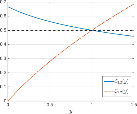
Figure 2.1: Functions $\mathcal{C}_{2,2}(y)$ and $\widetilde{\mathcal{C}}_{2,2}(y)$ for the class of explicit two-step, second-order perturbed LMM s. The dotted line shows $\widetilde{\mathcal{C}}_{\text{LMM}}=\mathcal{C}_{2,2}(1)$ for this particular class of methods.

For purely hyperbolic problems the spatial discretizations are usually chosen in such a way that $\bm{F}$ and $\widetilde{\bm{F}}$ satisfy (1.10) under the same step-size restriction. However, in many other cases (e.g. advection-reaction problems) this is not the case, as shown in Example 2.3. First, we mention the following lemma which is an extension of [1]; its proof can be found in Appendix A.

Lemma 2.4.

Consider the function

$$f(u)=\sum_{i=1}^{n}f_{i}(u)$$

and assume that there exist $\epsilon_{i}>0$ such that $||u+\tau f_{i}(u)||\leq||u||$ for $0\leq\tau\leq\epsilon_{i}$, $i\in\{1,\dots,n\}$, where $||\cdot||$ is a convex functional. Then $||u+\tau f(u)||\leq||u||$ for $0\leq\tau\leq\epsilon$, where

$$\epsilon=\left(\sum_{i=1}^{n}\frac{1}{\epsilon_{i}}\right)^{-1}.$$

Example 2.3.

Consider the LeVeque and Yee problem [14, 1]

$$U_{t}+f(U)_{x}=s(U),\quad U(x,0)=U_{0}(x),\quad x\in\mathbb{R},\,t\geq 0,$$

where $s(U)=-\mu U(U-1)(U-\frac{1}{2})$ and $\mu>0$. Let $u_{i}(t)\approx U(x_{i},t)$; then first-order upwind semi-discretization yields

$$u^{\prime}(t)=F(u(t))=D(u(t))+S(u(t)),\quad u(0)=u_{0},\quad t>0,$$

where

$$D_{i}(u)=-\frac{f(u_{i})-f(u_{i-1})}{\Delta x},\qquad S_{i}(u)=s(u_{i}).$$

Consider also the downwind discretizations

$$\widetilde{D}_{i}(u)=-\frac{f(u_{i+1})-f(u_{i})}{\Delta x},\qquad\widetilde{S}_{i}(u)=s(u_{i}),$$

and let $\widetilde{F}=\widetilde{D}+\widetilde{S}$. If $u\in[0,1]$, it can be easily shown that

$$0\leq u+\Delta t\,S(u)\leq 1\quad\text{for }0\leq\Delta t\leq\Delta t_{\textnormal{FE}}=\frac{2}{\mu},$$

$$0\leq u-\Delta t\,\widetilde{S}(u)\leq 1\quad\text{for }0\leq\Delta t\leq\widetilde{\Delta t}_{\textnormal{FE}}=\frac{16}{\mu}.$$

Using Lemma 2.4 we then have that

$$0\leq u+\Delta t\,F(u)\leq 1\quad\text{for }0\leq\Delta t\leq\Delta t_{\textnormal{FE}}=\frac{2\tau}{2+\mu\tau},$$

$$0\leq u-\Delta t\,\widetilde{F}(u)\leq 1\quad\text{for }0\leq\Delta t\leq\widetilde{\Delta t}_{\textnormal{FE}}=\frac{16\tau}{16+\mu\tau},$$

where $\tau>0$ is such that

$$0\leq u+\Delta t\,D(u)\leq 1\quad\text{for }0\leq\Delta t\leq\tau,$$

$$0\leq u-\Delta t\,\widetilde{D}(u)\leq 1\quad\text{for }0\leq\Delta t\leq\tau.$$

Note that $\Delta t_{\textnormal{FE}}<\widetilde{\Delta t}_{\textnormal{FE}}$ for all positive values of $\mu$ and $\tau$. Therefore, under assumptions (1) and (2) above, the forward Euler step size must be equal to $2\tau/(2+\mu\tau)$ so that the numerical solution is stable. Let $y=\Delta t_{\textnormal{FE}}/\widetilde{\Delta t}_{\textnormal{FE}}$, then for all $y<1$ we have $\widetilde{\mathcal{C}}_{\text{LMM}}=\mathcal{C}(1)<\mathcal{C}(y)$, hence not considering SSP perturbed LMM s will always result to a stricter step-size restriction. Suppose $\mu$ is relatively small so that the problem is not stiff and explicit methods could be used. For instance, among the class of explicit two-step, second-order LMMs, there is no classical SSP method and the optimal downwind method has SSP coefficient $\widetilde{\mathcal{C}}_{\text{LMM}}=1/2$. Let $\mu\tau=2/3$, then the step-size bound for downwind SSP methods such that the solution remains in $[0,1]$ is $\Delta t\leq 0.375\tau$. Using the optimal two-step, second-order SSP perturbed LMM larger step sizes are allowed since $\Delta t\leq\mathcal{C}(y)\,\Delta t_{\textnormal{FE}}=0.3929\tau$, where $y=\frac{16+\mu\tau}{8(2+\mu\tau)}$.

3 Monotonicity of additive linear multistep method s

Following the previous example, it is natural to study the monotonicity properties of additive methods applied to problems which consist of components that describe different physical processes. A $k$-step additive LMM for the solution of the initial value problem

$$\begin{split}\bm{u}^{\prime}(t)&=\bm{F}(\bm{u}(t))+\widehat{\bm{F}}(\bm{u}(t)),\quad t\geq t_{0}\\ \bm{u}(t_{0})&=\bm{u}_{0},\end{split}$$ (3.1)

takes the form

$$\bm{u}_{n}=\sum_{j=0}^{k-1}\alpha_{j}\bm{u}_{n-k+j}+\Delta t\sum_{j=0}^{k}\left(\beta_{j}\bm{F}(\bm{u}_{n-k+j})+\hat{\beta}_{j}\widehat{\bm{F}}(\bm{u}_{n-k+j})\right).$$ (3.2)

The method is explicit if $\beta_{k}=\hat{\beta}_{k}=0$. It can be shown that method (3.2) is order $p$ accurate if

$$\begin{gathered}\sum_{j=0}^{k-1}\alpha_{j}=1,\qquad\sum_{j=0}^{k-1}j\alpha_{j}+\sum_{j=0}^{k}\beta_{j}=k,\qquad\sum_{j=0}^{k-1}j\alpha_{j}+\sum_{j=0}^{k}\hat{\beta_{j}}=k,\\ \sum_{j=0}^{k-1}\alpha_{j}j^{i}+\sum_{j=0}^{k}\beta_{j}ij^{i-1}=k^{i},\quad\sum_{j=0}^{k-1}\alpha_{j}j^{i}+\sum_{j=0}^{k}\hat{\beta}_{j}ij^{i-1}=k^{i},\quad i\in\{2,\dots,p\}.\end{gathered}$$ (3.5)

The operators $\bm{F}$ and $\widehat{\bm{F}}$ generally approximate different derivatives and also have different stiffness properties. We extend the analysis of monotonicity conditions for LMMs by assuming that $\bm{F}$ and $\widehat{\bm{F}}$ satisfy

$$\|\bm{u}+\Delta t\bm{F}(\bm{u})\|\leq\|\bm{u}\|, \quad\forall\bm{u}\in\mathbb{R}^{m},\;0\leq\Delta t\leq\Delta t_{\textnormal{FE}},$$ (3.6a)

$$\|\bm{u}+\Delta t\widehat{\bm{F}}(\bm{u})\|\leq\|\bm{u}\|, \quad\forall\bm{u}\in\mathbb{R}^{m},\;0\leq\Delta t\leq\widehat{\Delta t}_{\textnormal{FE}},$$ (3.6b)

respectively.

Definition 3.1.

An additive LMM (3.2) is said to be strong stability preserving (SSP) if the following monotonicity conditions

$$\begin{split}\beta_{j},\hat{\beta}_{j}\geq 0,&\quad j\in\{0,\dots,k\},\\ \alpha_{j}-r\beta_{j}-\hat{r}\hat{\beta}_{j}\geq 0,&\quad j\in\{0,\dots,k-1\}.\end{split}$$ (3.7)

hold for $r\geq 0$ and $\hat{r}\geq 0$. For a fixed $y=\hat{r}/r$ the method has SSP coefficients $(\mathcal{C}(y),\widehat{\mathcal{C}}(y))$, where

$$\mathcal{C}(y)=\sup\bigl{\{}r\geq 0:\text{monotonicity conditions \eqref{eq:ALMMMonCond} hold with }\hat{r}=yr\bigr{\}}$$ (3.8)

and $\widehat{\mathcal{C}}(y)=y\,\mathcal{C}(y)$.

As in Section 2, it is clear that whenever the set in (3.8) is empty then the method is non-SSP; in such cases we say the method has SSP coefficient equal to zero.

Define the vectors $\bm{a}_{j},\bm{b}_{j}(x)\in\mathbb{R}^{p+1}$ as in (2.19) and (2.20). Then using the substitution

$$\gamma_{j}=\alpha_{j}-r\beta_{j}-\hat{r}\hat{\beta}_{j}\quad\text{for}\quad j\in\{0,\dots,k-1\},$$ (3.9)

the order conditions (3.5) can be expressed in terms of vectors $\bm{a}_{j},\bm{b}_{j}(x)$:

$$\sum_{j=0}^{k-1}(\gamma_{j}+\hat{r}\hat{\beta}_{j})\bm{a}_{j}+\sum_{j=0}^{k}r\beta_{j}\bm{b}_{j}(r^{-1})=\bm{a}_{k},$$ (3.10a)

$$\sum_{j=0}^{k-1}(\gamma_{j}+r\beta_{j})\bm{a}_{j}+\sum_{j=0}^{k}\hat{r}\hat{\beta}_{j}\bm{b}_{j}(\hat{r}^{-1})=\bm{a}_{k}.$$ (3.10b)

The above equations suggest a change of variables. Instead of considering the method’s coefficients in terms of the column vectors

$$\bm{\alpha}=(\alpha_{0},\dots,\alpha_{k-1})^{\intercal},\quad\bm{\beta}=(\beta_{0},\dots,\beta_{k})^{\intercal},\quad\bm{\hat{\beta}}=(\hat{\beta}_{0},\dots,\hat{\beta}_{k})^{\intercal},$$

and the order conditions independent of $r$ and $\hat{r}$, one can consider the coefficients $\bm{\gamma},\bm{\beta},\bm{\hat{\beta}}$ under the substitution (3.9). Let $\hat{r}=yr$. Then the order conditions can be written as functions of $r$. In particular the system of $p+1$ equations (3.10a) can be written as $A(r)\bm{x}(r)=\bm{a}_{k}$, where

$$A(r)=\left[\begin{array}[]{c|c|c|c|c|c|c}\bm{a}_{0}&\dots&\bm{a}_{k-1}&r\bm{b}_{0}(r^{-1})&\dots&r\bm{b}_{k-1}(r^{-1})&r\bm{b}_{k}(r^{-1})\\[10.00002pt] \end{array}\right]$$

and $\bm{x}(r)=\bigl{(}\bm{\delta}(r),\bm{\beta}\bigr{)}^{\intercal}\in\mathbb{R}^{2k+1}$ with $\delta_{j}(r)=\gamma_{j}+yr\hat{\beta}_{j}$, $j\in\{0,\dots,k-1\}$. Define the feasible set

$$P(r)=\{\bm{x}\in\mathbb{R}^{2k+1}:A(r)\bm{x}(r)=\bm{a}_{k},\;\bm{x}(r)\geq 0\}.$$ (3.11)

For a given $y$, if there exists a $k$-step, $p$-order accurate SSP additive LMM (3.2) with SSP coefficient $\mathcal{C}(y)$, then $P\bigl{(}\mathcal{C}(y)\bigr{)}$ is non-empty.

Since we would like to obtain the method with the largest possible SSP coefficient, then for a fixed $k\geq 1$, $p\geq 1$ and a given $y$, we define

$$\mathcal{C}_{k,p}(y)=\sup_{\bm{\alpha},\bm{\beta},\bm{\hat{\beta}}}\bigl{\{}\mathcal{C}(y)>0:\mathcal{C}(y)\text{ is the SSP coefficient of a $k$-step method \eqref{eq:ALMM} of order $p$}\bigr{\}}.$$

Definition 3.2.

Given $y$, an SSP $k$-step additive LMM (3.7) of order $p$ is called optimal if the order conditions (3.5) are satisfied and $\mathcal{C}(y)=\mathcal{C}_{k,p}(y)$.

Theorem 3.1.

Let $k\geq 1$, $p\geq 1$ be given such that $0<\mathcal{C}_{k,p}(y)<\infty$ for a given $y$. Then there exists a $k$-step optimal SSP additive LMM (3.2) of order $p$ with at most $p$ non-zero coefficients $\delta_{j},\beta_{i}$, where $\delta_{j}=\alpha_{j}-\mathcal{C}_{k,p}(y)\beta_{j}$, $j\in\{0,\dots,k-1\}$ and $i\in\{0,\dots,k\}$.

Proof.

Let $k\geq 1$, $p\geq 1$ and $y$ be given. Consider an optimal $k$-step SSP additive LMM (3.2) of order $p$ with SSP coefficient $\mathcal{C}_{k,p}(y)>0$. Define $\gamma_{j}=\alpha_{j}-\mathcal{C}_{k,p}(y)\beta_{j}-\hat{\mathcal{C}}_{k,p}(y)\hat{\beta}_{j}$ and $\delta_{j}=\gamma_{j}+\hat{\mathcal{C}}_{k,p}(y)\hat{\beta}_{j}$ for $j\in\{0,\dots,k-1\}$. Then the vector $\bm{x}=(\bm{\delta},\bm{\beta})^{\intercal}\in\mathbb{R}^{2K+1}$ belongs to the feasible set (3.11) when $r=\mathcal{C}_{k,p}(y)$.

Suppose $\bm{x}$ has at least $p+1$ non-zero coefficients and let $S$ be the set of columns of the matrix $A(r)$ in (3.11) corresponding to the non-zero elements of $x$. We distinguish two cases. First, assume that the set $S$ does not span $\mathbb{R}^{p+1}$. Then, similarly to the proof of Theorem 2.3, $x$ consists of at most $p$ non-zero elements. If now $S$ spans $\mathbb{R}^{p+1}$, let $\bm{x}_{p}=(\bm{x}_{B},\bm{x}_{N})^{\intercal}$ be a permutation of $\bm{x}$ such that $\bm{x}_{B}^{\intercal}\in\mathbb{R}^{p+1}$ is a strictly positive vector and $\bm{x}_{N}^{\intercal}\in\mathbb{R}^{2k-p}$ is non-negative. We can permute the columns of $A(r)$ in (3.11) in the same way, yielding $A_{p}(r)=[B(r)\;|\;N(r)]$, where $B\in\mathbb{R}^{(p+1)\times(p+1)}$ and $N\in\mathbb{R}^{(p+1)\times(2k-p)}$. Again, following the reasoning of the proof of Theorem 2.3, there exists $\epsilon>0$ such that $\bm{x}_{p}^{*}=(\bm{x}_{B}(\mathcal{C}_{k,p}(y)+\epsilon),\bm{x}_{N})^{\intercal}$ is a permutation of $\bm{x}^{*}=(\bm{\delta}^{*},\bm{\beta}^{*})^{\intercal}$ that solves $A(\mathcal{C}_{k,p}(y)+\epsilon)\bm{x}=\bm{a}_{k}$.

Moreover, for each index $j$ in $\bm{x}^{*}$ such that $\delta^{*}_{j}>0$, we can choose $\gamma^{*}_{j}$ so that $\beta^{*}_{j}=\hat{\beta}^{*}_{j}$. Then, $\bm{x}^{*}$ satisfies (3.10b) as well. But this contradicts to the optimality of the method since we have constructed a $k$-step SSP additive LMM of order $p$ with coefficients given by $\bm{x}^{*}$ and SSP coefficient $\mathcal{C}_{k,p}(y)+\epsilon$. ∎

Lemma 3.1.

For a given $k\geq 1,p\geq 1$ an optimal additive LMM (3.2) has $\beta_{j}=\hat{\beta}_{j}$ for all $j\in\{0,\dots,k\}$.

Proof.

Consider an optimal method (3.2) of order $p$. From Theorem 3.1 at most $p$ coefficients $\delta_{j},\beta_{i}$, $j\in\{0,\dots,k-1\}$, $i\in\{0,\dots,k\}$ are non-zero. Let $\bm{v}=\bm{\beta}-\bm{\hat{\beta}}$, then $\bm{v}$ has at most $p$ non-zero elements. Subtracting the order conditions (3.10) results in

$$\sum_{i\in I}v_{i}\bm{\bar{a}}_{i}=0,$$

where $I$ is the set of distinct indices for which $v_{i}$’s are non-zero. The vectors $\bm{\bar{a}}_{i}=(1,i,\dots,\allowbreak i^{p-1})^{\intercal}$, $i\in I$ are linearly independent (see [5, Chapter 21]), therefore $\bm{v}$ must be identically equal to zero. Hence, $\beta_{j}=\hat{\beta}_{j}$ for all $j\in\{0,\dots,k\}$. ∎

The main result of this section relies on Theorem 3.1 and Lemma 3.1.

Theorem 3.2.

For a given $k\geq 1,p\geq 1$ an optimal additive LMM with SSP coefficient $\mathcal{C}_{k,p}$ and corresponding SSP coefficient $\widehat{\mathcal{C}}_{k,p}$ is equivalent to the optimal $k$-step optimal SSP LMM (1.4) of order $p$ with SSP coefficient $\mathcal{C}_{k,p}+\widehat{\mathcal{C}}_{k,p}$.

Proof.

Consider an optimal method (3.2) of order $p$ with SSP coefficient $\mathcal{C}_{k,p}$ and $\widehat{\mathcal{C}}_{k,p}=y\,\mathcal{C}_{k,p}$ for some $y\in[0,\infty)$. From Lemma 3.1 we have $\beta_{j}=\hat{\beta}_{j}$ for all $j$, therefore monotonicity conditions (3.7) yield $\min_{j}\frac{\alpha_{j}}{\beta_{j}}=\mathcal{C}_{k,p}+\widehat{\mathcal{C}}_{k,p}$. Thus the additive LMM is equivalent to the optimal $k$-step SSP LMM method of order $p$ with SSP coefficient $\mathcal{C}_{k,p}+\widehat{\mathcal{C}}_{k,p}$. ∎

3.1 Monotone IMEX linear multistep method s

Based on Theorem 3.2, it is only interesting to consider Implicit-Explicit (IMEX) SSP linear multistep method s. Such methods are particularly useful for initial value problems (3.2) where $\bm{F}$ represents a non-stiff or mild stiff part of the problem, and $\widehat{\bm{F}}$ a stiff term for which implicit integration is required. The following theorem provides sufficient conditions for monotonicity for the numerical solution of an IMEX method.

Theorem 3.3.

Consider the additive problem (3.1) for which $\bm{F}$ and $\widehat{\bm{F}}$ satisfy (3.6), for some $\Delta t_{\textnormal{FE}}>0$ and $\widehat{\Delta t}_{\textnormal{FE}}>0$. Let an IMEX LMM (3.2) with coefficients $\beta_{k}=0$, $\hat{\beta_{k}}\neq 0$ be strong-stability-preserving with SSP coefficients $(\mathcal{C}(y),\widehat{\mathcal{C}}(y))$ for $y=\Delta t_{\textnormal{FE}}/\widehat{\Delta t}_{\textnormal{FE}}$. Then, the numerical solution satisfies the monotonicity condition (1.5) under a step-size restriction $\Delta t\leq\min\{\mathcal{C}\,\Delta t_{\textnormal{FE}},\widehat{\mathcal{C}}\,\widehat{\Delta t}_{\textnormal{FE}}\}$.

Proof.

The proof is similar to that of Theorem 2.1. ∎

As in the Section 2, the minimum step size in (3.3) occurs when $\mathcal{C}\,\Delta t_{\textnormal{FE}}=\widehat{\mathcal{C}}\,\widehat{\Delta t}_{\textnormal{FE}}$. For a given $k\geq 1$ and $p\geq 1$, we would like to find the largest possible value $\mathcal{C}_{k,p}(y)$ such that an optimal IMEX method is SSP with coefficients $(\mathcal{C}_{k,p},\mathcal{C}_{k,p}\,\Delta t_{\textnormal{FE}}/\widehat{\Delta t}_{\textnormal{FE}})$. Setting $y:=\Delta t_{\textnormal{FE}}/\widehat{\Delta t}_{\textnormal{FE}}$ and combining the inequalities (3.7) and the order conditions (3.5) we can form the following optimization problem:

$$\max_{\{\bm{\gamma},\bm{\beta},\bm{\hat{\beta}},r\}}\;r,\qquad\text{subject to}$$

$$\left\{\begin{array}[]{ll}\displaystyle\sum_{j=0}^{k-1}\gamma_{j}+r(\beta_{j}+y\hat{\beta}_{j})=1,\quad\displaystyle\sum_{j=0}^{k-1}\bigl{(}\gamma_{j}+r(\beta_{j}+y\hat{\beta}_{j})\bigr{)}j+\beta_{j}=k,&\\ \displaystyle\sum_{j=0}^{k-1}\bigl{(}\gamma_{j}+r(\beta_{j}+y\hat{\beta}_{j})\bigr{)}j^{i}+\beta_{j}ij^{i-1}=k^{i},&i\in\{2,\dots,p\},\\ \displaystyle\sum_{j=0}^{k-1}(\beta_{j}-\hat{\beta}_{j})-\hat{\beta}_{k}=0,\quad\displaystyle\sum_{j=0}^{k-1}(\beta_{j}-\hat{\beta}_{j})j^{i}-\hat{\beta}_{k}k^{i}=0,&i\in\{1,\dots,p-1\},\\ \gamma_{j}\geq 0,\beta_{j}\geq 0,&j\in\{0,\dots,k-1\},\\ \hat{\beta}_{j}\geq 0,&j\in\{0,\dots,k\},\\ r\geq 0.\end{array}\right.$$ (3.18)

By using bisection in $r$, the optimization problem (3.18) can be viewed as a sequence of linear feasible problems, as suggested in [10]. We solved the above problem using linprog in Matlab and found optimal IMEX SSP methods for $k\in\{1,\dots,40\},p\in\{1,\dots,15\}$ and for different values of $y$. Similarly to additive Runge–Kutta method s [6], we can define the feasibility SSP region of IMEX SSP methods for a fixed $k\geq 1$ and $p\geq 1$ by

$$R_{k,p}=\bigl{\{}(r,\hat{r}):y\in\mathbb{R}^{+}\text{ and monotonicity conditions \eqref{eq:ALMMMonCond} hold for }r\geq 0,\hat{r}=ry\bigr{\}}.$$

For instance, the feasibility SSP regions for three-step, second-order and six-step, fourth-order IMEX methods are shown in Figure 3.1.

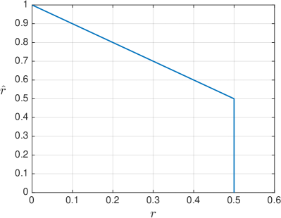
(a) Three-step, second-order IMEX SSP region

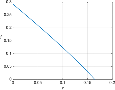
(b) Six-step, fourth-order IMEX SSP region

Figure 3.1: SSP regions of IMEX LMMs. Consider the half-line starting from the origin with a slope $y$ with the $r$-axis. Then, the intersection of the line $\hat{r}=yr$, $y>0$ with the boundary of the SSP region corresponds to an optimal IMEX LMM with SSP coefficient $\mathcal{C}(y)$.

As mentioned in [8, Section 2.1] the SSP coefficients of IMEX SSP methods in the case the forward Euler ratio $y=\Delta t_{\textnormal{FE}}/\widehat{\Delta t}_{\textnormal{FE}}$ is equal to one are not large. The same seems to hold when considering SSP IMEX methods for additive problems (3.1) satisfying (3.6) for any values $y\geq 0$ (see Figure 3.1). Thus, instead of requiring both parts of an IMEX method to be SSP, one can impose SSP conditions only on the explicit part and optimize stability properties for the implicit method. Second order methods among this class of methods have been studied in [2], whereas in [16] higher order IMEX methods with optimized stability features were constructed based on general monotonicity and boundedness properties of the explicit component.

4 Conclusion and future work

We have investigated a generalization of the linear multistep method s with upwind- and downwind-biased operators introduced in [17, 18], by considering problems in which the downwind operator satisfies a forward Euler condition with different step-size restriction than that of the upwind operator. We expressed the perturbed LMM s in an additive form and analyzed their monotonicity properties. By optimizing in terms of the upwind and downwind Euler step sizes, methods with larger SSP step sizes are obtained for such problems. We studied additive problems in the same framework, and we have shown that when both parts of the method are explicit (or both parts are implicit), the optimal additive SSP methods lie within the class of traditional (non-additive) SSP linear multistep methods. Finally, we have seen that IMEX SSP methods for additive problems allow relatively small monotonicity-preserving step sizes.

The concepts of additive splitting and downwind semi-discretization can be combined to yield downwind IMEX LMMs of the form (applying downwinding to the non-stiff term):

$$\bm{u}_{n}=\sum_{j=0}^{k-1}\alpha_{j}\bm{u}_{n-k+j}+\Delta t\sum_{j=0}^{k-1}\left(\beta_{j}\bm{F}(\bm{u}_{n-k+j})-\tilde{\beta}_{j}\widetilde{\bm{F}}(\bm{u}_{n-k+j})\right)+\Delta t\sum_{j=0}^{k}\hat{\beta}_{j}\widehat{\bm{F}}(\bm{u}_{n-k+j}),$$ (4.1)

where $\bm{F}$ and $\widetilde{\bm{F}}$ satisfy the forward Euler conditions (1.10) and the explicit part is an SSP perturbed LMM . Preliminary results show that it is possible to obtain second order IMEX linear multistep method s with two or three steps, where the implicit part is A-stable and the explicit part is an optimal SSP perturbed LMM . This generalization allows the construction of new IMEX methods with fewer steps for a given order of accuracy and with larger SSP coefficients (for the explicit component). Moreover, the best possible IMEX method can be chosen based on the ratio of forward Euler step sizes of the non-stiff term in (3.1). Also, it is worth investigating the possibility of obtaining A($\alpha$)-stable implicit parts whenever A-stability is not feasible. Work on optimizing the stability properties of the IMEX methods (4.1) is ongoing and will be presented in a future work. Analysis of SSP perturbed LMM s with variable step sizes and monotonicity properties of perturbed LMM s with special starting procedures can also be studied.

Acknowledgment

The authors would like to thank Lajos Lóczi and Inmaculada Higueras for carefully reading this paper and making valuable suggestions and comments.

Appendix

Appendix A Proofs of Lemmata in Section 2

In this section we present the proofs of some technical lemmata that were omitted in the previous sections.

Proof of Lemma 2.2.

Consider a set of distinct vectors $S=\{\bm{x}_{1},\dots,\bm{x}_{m}\}$ in $\mathbb{R}^{n}$. Let a non-zero vector $\bm{y}\in C$ be given. Then there exist non-negative coefficients $\lambda_{j}$ that sum to unity such that

$$\bm{y}=\sum_{j=1}^{m}\lambda_{j}x_{j}.$$

If $\bm{x}_{1},\dots,\bm{x}_{m}$ are linearly independent, it must be that $m\leq n$ and both parts (a) and (b) of the lemma hold trivially. Therefore, assume the vectors in $S$ are linearly dependent. Then, we can find $\mu_{j}$ not all zero and at least one which is positive, such that

$$\sum_{j=1}^{m}\mu_{j}\bm{x}_{j}=0.$$

Define

$$\nu=\min_{1\leq j\leq m}\left\{\frac{\lambda_{j}}{\mu_{j}}:\mu_{j}>0\right\}=\frac{\lambda_{j_{0}}}{\mu_{j_{0}}};$$

then we have $\nu\mu_{j}\leq\lambda_{j}$ for all $j\in\{1,\dots,m\}$, where equality holds for at least $j=j_{0}$. Let $\tilde{\lambda}_{j}=\lambda_{j}-\nu\mu_{j}$ for $j\in\{1,\dots,m\}$. By the choice of $\nu$, all coefficients $\tilde{\lambda}_{j}$ are non-negative and at least one of them is equal to zero. Note that

$$\bm{y}=\sum_{j=1}^{m}\lambda_{j}\bm{x}_{j}-\nu\sum_{j=1}^{m}\mu_{j}\bm{x}_{j}=\sum_{j=1}^{m}\tilde{\lambda}_{j}\bm{x}_{j},$$

hence $\bm{y}$ can be expressed as a non-negative linear combination of at most $m-1$ vectors in $S$. The above argument can be repeated until $\bm{y}$ is written as a non-negative linear combination of $\bm{x}_{1},\dots,\bm{x}_{r}$ linearly independent vectors, where $r\leq n$. This proves part (a).

For part (b), suppose $\bm{x}_{1},\dots,\bm{x}_{m}$ are linearly dependent and belong in $\{(1,\bm{v}):\bm{v}\in\mathbb{R}^{n-1}\}$. Then, any non-zero vector $\bm{y}\in C$ has the form $(1,\bm{v})^{\intercal}$, $\bm{v}\in\mathbb{R}^{n-1}$ and from part (a) can be written as a non-negative combination of at most $n$ linearly independent vectors in $S$ with coefficients $\tilde{\lambda}_{j}$. In addition $\sum_{j=1}^{m}\tilde{\lambda}_{j}=1$, since the first component of all $\bm{x}_{j}$ and $\bm{y}$ is one. ∎

Proof of Lemma 2.4.

Let $p_{i}(u;\epsilon_{i}):=u+\epsilon_{i}f_{i}(u)$, then we have

$$f_{i}(u)=\frac{p_{i}(u;\epsilon_{i})-u}{\epsilon_{i}},\quad\text{for }i\in\{1,\dots,n\}.$$

Using $\sum_{i=1}^{n}\epsilon/\epsilon_{i}=1$ and the assumption of the lemma, it can be shown that

$$\|u+\epsilon f(u)\| =\left\|u+\sum_{i=1}^{n}\frac{\epsilon}{\epsilon_{i}}\left(p_{i}(u;\epsilon_{i})-u\right)\right\|$$

$$=\left\|\sum_{i=1}^{n}\frac{\epsilon}{\epsilon_{i}}p_{i}(u;\epsilon_{i})\right\|$$

$$\leq\sum_{i=1}^{n}\frac{\epsilon}{\epsilon_{i}}\|u\|=\|u\|.$$

The rest of the proof relies on [15, Lemma II.5.1]. If $0\leq\tau<\epsilon$, then there exist $0<\rho<1$ such that $\tau=(1-\rho)\epsilon$. Then $u+\tau f(u)=u+(1-\rho)\epsilon f(u)=\rho u+(1-\rho)\left(u+\epsilon f(u)\right)$ and hence

$$\|u+\tau f(u)\|-\|u\| \leq\rho\|u\|+(1-\rho)\|u+\epsilon f(u)\|-\|u\|$$

$$=\left(1-\rho\right)\left(\|u+\epsilon f(u)\|-\|u\|\right)$$

$$\leq\|u+\epsilon f(u)\|-\|u\|.$$

This implies that $\|u+\tau f(u)\|\leq\|u+\epsilon f(u)\|$, whenever $0\leq\tau\leq\epsilon$ and the result follows. ∎

References

- [1] R. Donat, I. Higueras and A. Martínez-Gavara “On stability issues for IMEX schemes applied to 1D scalar hyperbolic equations with stiff reaction terms” In Math. Comp. 80.276, 2011, pp. 2097–2126 DOI: 10.1090/S0025-5718-2011-02463-4
- [2] Thor Gjesdal “Implicit-explicit methods based on strong stability preserving multistep time discretizations” In Appl. Numer. Math. 57.8, 2007, pp. 911–919 DOI: 10.1016/j.apnum.2006.09.001
- [3] Sigal Gottlieb, David I Ketcheson and Chi-Wang Shu “Strong Stability Preserving Runge–Kutta and Multistep Time Discretizations” World Scientific, 2011 URL: http://scholar.google.com/scholar?q="STRONG+STABILITY+PRESERVING+RUNGE-KUTTA+AND+MULTISTEP+TIME+DISCRETIZATIONS"&hl=en&btnG=Search&as\_sdt=1,5&as\_sdtp=on#0
- [4] Sigal Gottlieb and Steven J. Ruuth “Optimal strong-stability-preserving time-stepping schemes with fast downwind spatial discretizations” In Journal of Scientific Computing 27.1-3, 2006, pp. 289–303 DOI: 10.1007/s10915-005-9054-8
- [5] Nicholas J. Higham “Accuracy and Stability of Numerical Algorithms” SIAM, 2002 URL: http://www.amazon.com/Accuracy-Stability-Numerical-Algorithms-Nicholas/dp/0898715210%3FSubscriptionId%3D0JYN1NVW651KCA56C102%26tag%3Dtechkie-20%26linkCode%3Dxm2%26camp%3D2025%26creative%3D165953%26creativeASIN%3D0898715210
- [6] Inmaculada Higueras “Strong stability for additive Runge–Kutta methods” In SIAM Journal on Numerical Analysis 44.4, 2006, pp. 1735–1758 DOI: 10.1137/040612968
- [7] Inmaculada Higueras “Positivity properties for the classical fourth order Runge-Kutta method” In Monografías de la Real Academia de Ciencias de Zaragoza 33, 2010, pp. 125–139 URL: http://www.unizar.es/acz/05Publicaciones/Monografias/MonografiasPublicadas/Monografia33/125.pdf
- [8] Willem Hundsdorfer and Steven J. Ruuth “IMEX extensions of linear multistep methods with general monotonicity and boundedness properties” In Journal of Computational Physics 225.2, 2007, pp. 2016–2042 DOI: 10.1016/j.jcp.2007.03.003
- [9] Willem Hundsdorfer, Steven J. Ruuth and Raymond J. Spiteri “Monotonicity-preserving linear multistep methods” In SIAM J. Numer. Anal. 41.2, 2003, pp. 605–623 DOI: 10.1137/S0036142902406326
- [10] David I. Ketcheson “Computation of optimal monotonicity preserving general linear methods” In Mathematics of Computation 78.267, 2009, pp. 1497–1513 DOI: 10.1090/S0025-5718-09-02209-1
- [11] David I. Ketcheson “Step sizes for strong stability preservation with downwind-biased operators” In SIAM Journal on Numerical Analysis 49.4, 2011, pp. 1649–1660 DOI: 10.1137/100818674
- [12] H. W. J. Lenferink “Contractivity preserving explicit linear multistep methods” In Numerische Mathematik 55.2, 1989, pp. 213–223 DOI: 10.1007/BF01406515
- [13] H. W. J. Lenferink “Contractivity-preserving implicit linear multistep methods” In Math. Comp. 56.193, 1991, pp. 177–199 DOI: 10.2307/2008536
- [14] R. J. LeVeque and H. C. Yee “A study of numerical methods for hyperbolic conservation laws with stiff source terms” In J. Comput. Phys. 86.1, 1990, pp. 187–210 DOI: 10.1016/0021-9991(90)90097-K
- [15] Robert Harold Martin “Nonlinear Operators and Differential Equations in Banach Spaces (Pure & Applied Mathematics Monograph)” John Wiley & Sons Inc, 1976 URL: http://www.amazon.com/Nonlinear-Operators-Differential-Equations-Mathematics/dp/0471573639%3FSubscriptionId%3D0JYN1NVW651KCA56C102%26tag%3Dtechkie-20%26linkCode%3Dxm2%26camp%3D2025%26creative%3D165953%26creativeASIN%3D0471573639
- [16] Steven J. Ruuth and Willem Hundsdorfer “High-order linear multistep methods with general monotonicity and boundedness properties” In J. Comput. Phys. 209.1, 2005, pp. 226–248 DOI: 10.1016/j.jcp.2005.02.029
- [17] Chi-Wang Shu “Total-variation-diminishing time discretizations” In SIAM Journal on Scientific and Statistical Computing 9.6, 1988, pp. 1073–1084 DOI: 10.1137/0909073
- [18] Chi-Wang Shu and Stanley Osher “Efficient implementation of essentially nonoscillatory shock-capturing schemes” In Journal of Computational Physics 77.2, 1988, pp. 439–471 DOI: 10.1016/0021-9991(88)90177-5