An HST Proper-Motion Study of the Large-scale Jet of 3C273

Abstract

The radio galaxy 3C 273 hosts one of the nearest and best-studied powerful quasar jets. Having been imaged repeatedly by the Hubble Space Telescope (HST) over the past twenty years, it was chosen for an HST program to measure proper motions in the kiloparsec-scale resolved jets of nearby radio-loud active galaxies. The jet in 3C 273 is highly relativistic on sub-parsec scales, with apparent proper motions up to 15$c$ observed by VLBI (Lister et al., 2013). In contrast, we find that the kpc-scale knots are compatible with being stationary, with a mean speed of $-$0.2$\pm$0.5$c$ over the whole jet. Assuming the knots are packets of moving plasma, an upper limit of $1c$ implies a bulk Lorentz factor $\Gamma<$2.9. This suggests that the jet has either decelerated significantly by the time it reaches the kpc scale, or that the knots in the jet are standing shock features. The second scenario is incompatible with the inverse Compton off the Cosmic Microwave Background (IC/CMB) model for the X-ray emission of these knots, which requires the knots to be in motion, but IC/CMB is also disfavored in the first scenario due to energetic considerations, in agreement with the recent finding of Meyer & Georganopoulos (2014) which ruled out the IC/CMB model for the X-ray emission of 3C 273 via gamma-ray upper limits.

1. Introduction

About 10% of active galactic nuclei (AGN) produce bipolar jets of relativistic plasma which can reach scales of tens to hundreds of kiloparsecs in extent. While there is growing evidence that AGN feedback, including jet production, may have an important impact on galaxy and cluster evolution (e.g. Fabian, 2012), uncertainties about the physical characteristics of these jets has encumbered attempts to make these impacts understood quantitatively. Among the chief open questions are the identity of the radiating particles (positrons, electrons, or hadronic species), the lifetimes and duty cycles of the jets, and the magnetic field strength and speed of the plasma. All of these characteristics feed into the calculation of how much energy and momentum are carried by these jets and ultimately deposited into the galaxy and/or cluster-scale environment.

In theory, proper-motion studies allow us to put direct constraints on the speed of AGN jets, and consequently their Lorentz factors ($\Gamma$). Hundreds of observations of jets with very long baseline interferometry (VLBI) in the radio have detected proper motions of jets on parsec and sub-parsec scales, relatively near to the black hole engine (e.g. Kellermann et al., 1999; Giovannini et al., 2001; Jorstad et al., 2001; Piner & Edwards, 2004; Kellermann et al., 2004; Jorstad et al., 2005; Lister et al., 2009; Piner et al., 2010). These observations show that these jets are often highly relativistic, such that velocities near the speed of light coupled with relatively small viewing angles result in apparent superluminal motion. The dimensionless observed apparent velocity $\beta_{\mathrm{app}}$ is related to the real velocity $\beta=v/c$ (where $c$ is the speed of light) and viewing angle $\theta$ through the well-known Doppler formula $\beta_{\mathrm{app}}=\beta\sin\theta/(1-\beta\cos\theta)$. A measurement of $\beta_{\mathrm{app}}$ implies both a lower limit on the Lorentz factor ($\Gamma_{\mathrm{min}}\approx\beta_{\mathrm{app}}$) and an upper limit on the viewing angle – constraints which are very difficult to derive using other means such as spectral fitting, due to the inherent degeneracy between intrinsic power, angle, and speed introduced by Doppler boosting of the observed flux.

While proper motions of jets on parsec scales exist in large samples, direct observations of jet motions on much larger scales (kpc-Mpc) are rare. Such observations naturally rely on sub-arcsecond resolution telescopes like the Very Large Array (VLA), Atacama Large Millimeter/submillimeter Array (ALMA), or Hubble Space Telescope (HST) in order to image the full jet in detail, but this (much lower than VLBI) resolution necessarily also limits potential observations of apparent motions to sources in the very local Universe, and require years or even decades of repeated observations. Superluminal motions on kpc scales also might not be common, as the jet presumably decelerates as it extends out from the host galaxy, though it must be at least mildly relativistic to explain jet one-sidedness. Statistical studies of jet-to-counterjet ratios in the radio generally suggest that kpc-scale quasar jets are only mildly relativistic ($\Gamma\sim few,$ Arshakian & Longair, 2004; Mullin & Hardcastle, 2009).

A common problem for both VLBI-scale and kpc-scale proper-motion studies is the interpretation of slow-moving or stationary features in jets. While observed motions imply a corresponding minimum bulk speed, fast bulk speeds could also be present in jets that do not produce convenient ballistic features which can be easily tracked, and stationary or slow-moving features may instead correspond to stationary shocks within the flow. An obvious example is the famous knot HST-1 in the jet of M87, which is thought to be a standing recollimation shock, through which plasma is moving with a moderately relativistic bulk speed (Biretta et al., 1999; Stawarz et al., 2006; Cheung et al., 2007). A similar feature has been seen in the radio in 3C 120 (Agudo et al., 2012). On VLBI scales, stationary features can also appear in jets along with moving components. Some two-thirds of the objects in the VLBI proper motions study of BL Lacs by Jorstad et al. (2001) contained stationary features, a common finding in VLBI studies generally (e.g., Alberdi et al., 2000; Lister et al., 2009).

For many years, there were only two measured proper motions of jets on kpc scales, both taken with the VLA. These were the famous result of $\beta_{\mathrm{app}}$ up to $6c$ measured by Biretta et al. (1995) for the jet in M87 (z=0.004, d=22 Mpc), and a speed of $\approx 4c$ for a knot in the jet in 3C 120 (z=0.033, d=130 Mpc) by Walker et al. (1988), though this was later contradicted by additional VLA and Merlin observations (Muxlow & Wilkinson, 1991; Walker, 1997). In 1999, the first measurement of proper motions in the optical was accomplished by Biretta et al. (1999), using four years of HST Faint Object Camera (FOC) imaging to confirm the fast superluminal speeds in the inner jet of M87. However, until recently (Meyer et al., 2013) it was unclear if M87 would prove to be the only superluminal jet on kpc scales.

With the continued development of high-precision astrometry techniques to align HST images, it is now possible to register images of jets repeatedly observed by HST over the past 20 or more years for proper motions studies. With a single moderately deep HST image, it is possible to build a reference frame using background or stationary sources on which to register previous archival imaging to high precision. In many cases, the longest baselines are supplied by the early WFPC2 snapshot programs which targeted bright radio galaxies from 1994 through 1998 (e.g., HST programs 5476, 5980, 6363). The first successful application of high-precision HST astrometric methods to jet proper motions was done for the jet in M87, where we were successful in matching over 400 raw images of the jet taken from 1995 through 2008 using globular clusters in the host galaxy (Meyer et al., 2013). The Meyer et al. (2013) study greatly improved on previous efforts both in lengthening the time baseline and in reaching errors on the speed measurements as low as 0.1$c$, allowing us to measure both transverse motions and decelerations for the first time.

Figure 1.— Upper Panel: The immediate environment of 3C 273 as seen in the ACS/WFC reference image from 2014. The intensity has been scaled to emphasize the background sources, so the jet appears overexposed (center). The host galaxy/jet core is the extremely bright source at right. The thirteen galaxies used in the registration of the 1995 epoch are shown, boxed. The larger box outline is roughly the field of view for the PC chip in 1995. Lower Panel: View of the 3C 273 optical jet after galaxy light subtraction. Knots are labeled according to standard convention, as well as several nearby background galaxies.

In the Meyer et al. (2013) study of M87, we reached a limiting astrometric precision in measuring the positions of knots in the jet of a few mas or less. Over a twenty year baseline, this translates into a distance limit of $\approx$600 Mpc, for a target accuracy of 1$c$ in the measurement of superluminal motion. The handful of optical jets within this local volume which were first observed in the 1990s are thus ripe targets for HST proper motions studies. Based on the success of the Meyer et al. (2013) study, we were awarded ACS/WFC observations in cycle 21 for 3 additional nearby jets previously imaged by HST, including 3C 273, the results of which are presented here. The results for accompanying target 3C 264, a jet similar to M87 but 5 times more distant, were published in Meyer et al. (2015b), while those for 3C 346 will be published separately.

At a redshift of 0.158 (d = 567 Mpc), 3C 273 is the furthest kpc-scale proper-motions target yet attempted with HST. The large-scale jet extends nearly 23^′′ from the core (see Figure 1) and has been observed extensively from radio to X-rays over the past few decades (e.g., Schmidt et al., 1978; Conway et al., 1981; Tyson et al., 1982; Lelievre et al., 1984; Harris & Stern, 1987; Thomson et al., 1993; Bahcall et al., 1995; Jester et al., 2001; Marshall et al., 2001; Sambruna et al., 2001; Jester et al., 2005, 2006; Uchiyama et al., 2006; Jester et al., 2007). The X-ray jet of 3C 273 is one of a group of “anomalous” X-ray jets discovered by Chandra, where the X-ray emission is too hard and at too high a level to be consistent with the known radio-optical synchrotron spectrum (Jester et al., 2006). The generally favored model up until very recently was that these X-rays were produced by inverse Compton upscattering of CMB photons by a jet still highly relativistic on kpc scales, to match high speeds implied by parsec-scale VLBI proper motions (Tavecchio et al., 2000; Celotti et al., 2001). As we discuss in this paper, this model implies that the knots in jets like 3C 273 should move with significant proper motions. However, the IC/CMB model was recently ruled out based on gamma-ray upper limits (Meyer & Georganopoulos, 2014), a method first described in Georganopoulos et al. (2006), and the strong upper limits placed by our proper motion observations as described in this paper also strongly disfavor an IC/CMB origin for the X-rays in 3C 273.

Table 1HST Imaging Data

Epoch	PID	Instrument	Date	Filter	Exp.	No.
			(mm/year)		(s)
1995	59807	WFPC2/PC	06/1995	F622W	2300	1
					2500	1
					2600	2
2003	90697	WFPC2/PC	04/2003	F622W	1100	2
					1300	6
2014	13327	ACS/WFC	05/2014	F606W	0550	4
					0598	12

The paper is organized as follows: in Section 2 we present our methods including use of background galaxies to register the images; in Section 3 we present the resulting proper-motion limits, and in Section 4 we discuss the implications that slow speeds have for our understanding of the physical conditions in the outer 3C 273 jet. In Section 5 we summarize our conclusions.

2. methods

The data used for this project is summarized in Table 1, where we list the project number, instrument setup, date of observation, and exposure time(s) for the individual exposures, organized into epochs. Only the 1995 imaging has been previously reported in Jester et al. (2001). We limited the study to observations in ‘V-band’ F606W or F622W filters (noting that the wavelength range of the latter is entirely within the range of the former) for consistency.

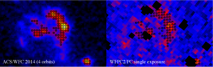
Figure 2.— At left, galaxy No. 2 from Figure 1 as seen in the ACS reference image. The black points are a portion of the ‘sampling grid’ described in the text, which sample the flux distribution of the galaxy. At right, the same galaxy in a single exposure (jca201l2q) from the 1995 WFPC2/PC set. The reference grid has been transformed based on an initial solution into the coordinates of the raw exposure, as shown. A flux-level cut was applied to only select the grid points falling on the brightest parts of the image, so that the positions can be compared more easily. Note that the black areas in the right image are locations of cosmic ray artifacts, where flux is set to equal zero to make the image more clear.

Before analyzing the archival WFPC2 data, each raw image was separately corrected for CTE losses. These losses are increasingly significant in WFPC2 data with time; we found that without making such a correction the fluxes measured in the jet and background galaxies were underestimated by $\approx$5 and $\approx 15$% in the 1995 and 2003 stacks, compared with the ACS deep stack. The correction was done pixel-by-pixel since the jet is resolved and losses depend on the x and y location on the detector; the method of calculating the correction maps is described in Appendix A. Note that the CTE correction was not found to have any effect on image registration or measurement of proper motions.

2.1. Reference Image

The four orbits of ACS/WFC imaging obtained in May of 2014 were stacked into a mean reference image (with cosmic-ray rejection) on a super-sampled scale with 0.025^′′ pixels. The registration of the 8 individual exposures utilized a full 6-parameter linear transformation based on the distortion-corrected positions of 15-20 point-like sources. The median one-dimensional rms residual relative to the mean position was 0.07 reference-frame pixels, or 1.75 mas, corresponding to a systematic error on the registration ($\times 1/\sqrt{1}6$) of 0.44 mas, or about 2 hundredths of a pixel.

The final science image was scaled to monochromatic flux at 6000 Å , where the PHOTFLAM value was recalculated in IRAF/STSDAS package calcphot with a power-law model, $\nu^{-1}$, in keeping with the spectral index reported in Jester et al. (2001). We also included a reddening/extinction correction with E(B-V)=0.018 for the position of 3C 273 as derived from the publicly available online DUST tool.

2.2. Background Source Registration

To create the 1995 and 2003 epoch science images, an astrometric solution was found between each individual (geometrically-corrected) exposure and the reference frame based on the 2014 ACS image. Typically, this is accomplished by identifying background point sources in the deep reference image which constitute the reference frame of sources used to register the prior epochs. While some globular clusters associated with the 3C 273 host galaxy can be seen in the deep ACS image, these are not detected in the much noisier PC imaging. Instead, we identified 18 background galaxies based on the criteria that they can be seen by eye above the noise in the individual PC exposures. These reference galaxies are highlighted in Figure 1. Note that galaxies 4, 5, and 6 have been previously identified as unrelated to the jet by their lack of radio emission, and the bright point source near the jet is actually a foreground star (and thus unsuitable for registering images due to likely proper motions).

To match the archival images to a common reference frame, our general strategy was to use the shape and light distribution of the galaxy to assist in matching their locations in each image. Instead of identifying a single location associated with each galaxy in the deep reference image, we instead sample the galaxy in a grid pattern, resulting in a list of positions along with the flux at each point, sampling across each galaxy. For example, we show at left in Figure 2 one of the background galaxies from the deep 2014 image. Grid points are placed at pixel centers, where we show only those where the pixel value is $>$10 times the background for illustration. At right, we have used an initial transformation solution to map the points to locations on the galaxy in a single raw frame. The flux at each point is interpolated based on nearby pixels.

We used the geometric correction solutions to first create geometrically-corrected (GC) images from the individual exposures. An initial (astrometric) transformation solution was found by supplying $\approx$10 pairs of matched locations found by hand between the GC image and the ACS reference image and calculating the six transformation parameters (without match evaluation/rejection). This initial transformation solution was then used to create a ‘rough’ mean image stack for each epoch (in counts units). This stacked image was then ‘reverse-transformed’ to create a reference image on the scale of each individual (distorted) raw exposure, in order to detect cosmic rays. These were detected by initially looking for pixels at a high (10$\sigma$) deviation from the reference image value, and then masking all adjacent pixels until all surrounding pixels are near to the mean value for that pixel. A mask for all pixels flagged as cosmic rays (as well as for a bad row at x=339 in the 1995 exposures) was thus created for each raw exposure.

2.3. Optimizing the Transformation

The initial transformation solution described above is used as a starting point to transform the x,y locations for each galaxy grid in the reference frame into $x_{gc},y_{gc}$ location in the geometrically corrected image as shown in and discussed previously for Figure 2. The intensity can then be sampled at each location in the GC image, to be compared directly to the scaled counts value predicted by the scaled reference pixel value. For each galaxy in each individual (GC) exposure, we shift the $x_{gc},y_{gc}$ over a grid of $\delta$x, $\delta$y values, in steps of 1/10th of a pixel for a total testing range of $\pm$2 pixels. At each point in the grid, a ‘score’ equal to the sum of squared differences is calculated for the sampling grid (dropping points falling on cosmic ray artifacts) based on the updated $x_{gc},y_{gc}$ positions in the GC image. We then fit the score matrix with a 2-dimensional Gaussian using IDL routine 2DGAUSSFIT in order to find the value of $\delta$x, $\delta$y corresponding to a globally consistent minimum which corresponds to the optimal position shift which is used to update the location of the galaxy in the reference frame.

For each individual exposure, we then compile an updated list of position matches between the reference frame and the GC image from the mean x,y value of the galaxy sampling grid in each. In general, we used a subset of the background galaxies which were identifiable by eye and not overly affected by cosmic ray hits. The process of finding the initial $x_{gc},y_{gc}$ values, followed by finding the optimal $\delta$x,$\delta$y improvement on the mean position, was iterated until the positions of galaxies stopped improving.

Figure 3.— The jet of 3C 273 as seen in 1995, 2003, and 2014. The first two images were taken with the WFPC2/PC, the most recent with the ACS/WFC. All have been scaled to monochromatic flux at 6000 Angstroms (white = 0.01 $\mu Jy$) after CTE correction, and background and host galaxy light subtraction. As shown, no changes in the jet are readily apparent by eye. The bright foreground star below knots D and C3 does appear to move with a speed of about 2 mas/year. Note that we follow the knot labeling of (Marshall et al., 2001).

The final science image stacks at each epoch have been scaled to monochromatic flux at 6000 $\AA$, with background and host galaxy light subtracted, and are shown in Figure 3. Note that we use the knot labeling originally defined in Marshall et al. (2001) and not the later, different labeling used in Uchiyama et al. (2006) and Jester et al. (2007).

2.4. Measuring Speeds

We employed two methods to measure the positions of the 10 individual knots, as well as the 4 background galaxies and foreground star identified in Figure 1, in each of the three epochs. First, similar to the methods employed in the studies of M87 and 3C 264 (Meyer et al., 2013, 2015b), we used a centroid position (flux-weighted mean $x$ and $y$ location) inside a contour surrounding the brightest part of the knot (hereafter referred to as the ‘contour method’). For the brighter knots (A1, B1, D and H3), we used the 50% peak flux-over background contour as measured using a cosine-transform representation of the image. For the fainter knots where the flux is only slightly higher than the local background (making it difficult to form a closed contour), we simply used a fixed circular aperture, centered on the brightest part of the knot (radius of the aperture depends on the size of the feature and is given in Table 2).

As a consistency check, we also measured the shift of each knot using a second method which we refer to as the ‘cross-correlation’ method. Over a grid with sub-pixel spacing of 0.2 super-sampled pixels (5 mas), we shifted the 1995 and 2003 images of each individual knot relative to the 2014 image (same cutout area) over a 6x6 pixel area, evaluating the sum of the squared differences between interpolated flux over the knot area for each x/y shift combination. The resulting sum-of-squared differences image in all cases clearly shows a smooth ‘depression’ feature which is reasonably well-fit by a two-dimensional Gaussian under the transformation $g=1-f/\mathrm{max}(f)$, where $f$ is the original sum of squared differences. Taking the minimum $f$ location as measured by the peak of the two-dimensional Gaussian fit, we measure the optimal shift for each knot.

To measure the approximate error on the positions measured, we repeated both of the above methods for simulated images of the jet at each epoch. The simulated images were created by taking the deep 2014 ACS image and adding a Gaussian noise component appropriately scaled from the counts in the original WFPC2 exposures. Since the 2014 image itself has some noise, and also a slightly different PSF from the WFPC2 images, this method likely slightly overestimates the errors. We take the error on each knot measurement to be the standard deviation of the measurements in the simulated images (10 in each epoch).

Finally, we plotted the position of each feature relative to the 2014 position, versus time, to look for evidence of proper motions. We have transformed from the coordinate frame of the aligned images (North up) to one based on the jet, where positive $x$ is in the outflow direction along the jet (taken as position angle (PA) 42^∘ south of east) and positive $y$ is orthogonal and to the north of the jet. The data are listed in table 2 and plotted in Figures 4 and 5. For both methods, the estimated error on the measurement has been convolved with the systematic error of the registration, which is 0.18, 0.22, and 0.02 reference pixels (4.5, 2.8, and 0.5 mas) for the 1995, 2003, and 2014 epochs, respectively.

3. Results

We first show in Figure 3 a comparison of the jet of 3C 273 in each epoch, where the background and host galaxy light has been subtracted, and the jet rotated to horizontal. No obvious changes in the jet are discernible by eye, and the fluxes of all components (as well as background sources) are consistent to within 5%. The only moving component, easily seen when blinking the 1995 and 2014 images against one another, is the foreground star near knot C3, which exhibits an apparent motion of 1.9 mas/year, at an angle of 20^∘ north of the the jet direction (where the jet PA is 222^∘). The proper motion is typical for disk stars in our own galaxy (e.g., Deason et al., 2013), and the star has a V-band magnitude of 25.6 (STMAG system) and color $m_{F606W}-m_{F814W}$ = 2.9, consistent with the source being a milky way foreground star.

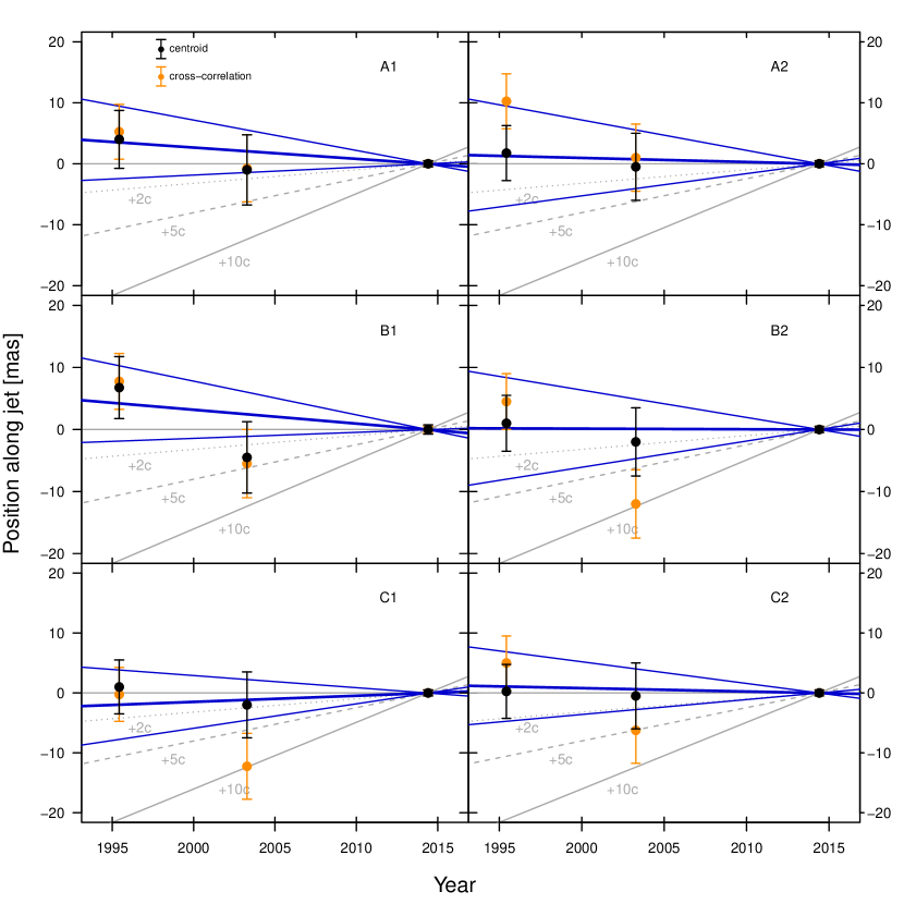
Figure 4.— Shift of individual knots (name noted at upper right of each panel) versus time relative to the 2014 measured position. Black points represent the contour-derived shifts and orange points the cross-correlation derived shifts. As a guide, lines corresponding to an apparent forward speed of 2$c$ (dotted gray) and 5$c$ (dashed gray) and 10$c$ (solid gray) are plotted in each subfigure. The thick solid blue line is the best-fit weighted linear regression model to all points, while the thinner blue lines show the 2$\sigma$ (95%) upper and lower limit slopes.

In Figures 4 and 5, we have plotted the shift of each knot relative to 2014 versus time, where black points represent the contour-derived shifts and orange points the cross-correlation derived shifts. As a guide, lines corresponding to an apparent forward speed of 2$c$ (dotted gray) and 5$c$ (dashed gray) and 10$c$ (solid gray) are plotted in each subfigure. The thick solid blue line is the best-fit weighted linear regression model to all points, while the thinner blue lines show the 2$\sigma$ (95%) upper and lower limit slopes. While the two methods of measuring shifts agree well for most knots, the deviation of the cross-correlation method from the contour method increases with decreasing surface brightness. We have thus excluded the cross-correlation derived points from the linear fitting for the two knots of particularly low surface brightness, A2 and B2, though these points are still plotted in orange in Figure 4.

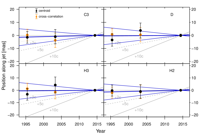
Figure 5.— Shift of individual knots (name noted at upper right of each panel) versus time relative to the 2014 measured position. Black points represent the contour-derived shifts and orange points the cross-correlation derived shifts. As a guide, lines corresponding to an apparent forward speed of 2$c$ (dotted gray) and 5$c$ (dashed gray) and 10$c$ (solid gray) are plotted in each subfigure. The thick solid blue line is the best-fit weighted linear regression model to all points, while the thinner blue lines show the 2$\sigma$ (95%) upper and lower limit slopes.

In Table 3 we report the results of the weighted linear regression fit to the position measurements for the 10 identified knots in Figure 1, as well as four nearby background galaxies and the foreground star near knot C3. In column 1 we give the knot or object name, in column 2 the measured flux of the knot in $\mu$Jy, in column 3 the aperture used to measure the surface brightness given in column 4 in $\mu$Jy/arcsec². In columns 5 and 6 we give the measured angular speed in mas yr^-1 in the $x$ (along the jet) and $y$ (perpendicular to jet) directions, and in columns 7 and 8 the corresponding apparent speeds $\beta_{app,X}$, $\beta_{app,Y}$ in units of $c$, using the conversion factor 8.9856 $c$/(mas yr^-1). While these latter values are incorrect/unphysical for the four galaxies and foreground star (as they are at different/unknown distances), we include the conversion to $\beta_{app}$ in Table 3 as a convenient reference for the accuracy of our measurements, since these sources should be completely stationary. In column 9 we give the probability that the speed of the knot is greater than zero, and in the final column the 99% upper limit on $\beta_{app,X}$.

As shown, all knots have speeds consistent with zero within the errors of our measurements. The mean speed along the jet, combining all knot values in column 7, is $-0.2\pm 0.5c$ As an additional check, we ran a cross-correlation analysis as described above for individual knots for the entire optical jet region. The best-fit weighted linear regression line yielded a slope of $-$0.006$\pm$0.22 mas yr^-1 and 0.12$\pm$0.22 mas yr^-1 along and perpendicular to the jet, and corresponding to apparent speeds of $-$0.04$\pm$1.9$c$ and 1.1$\pm$1.9$c$, respectively, also consistent with a speed of zero in both directions.

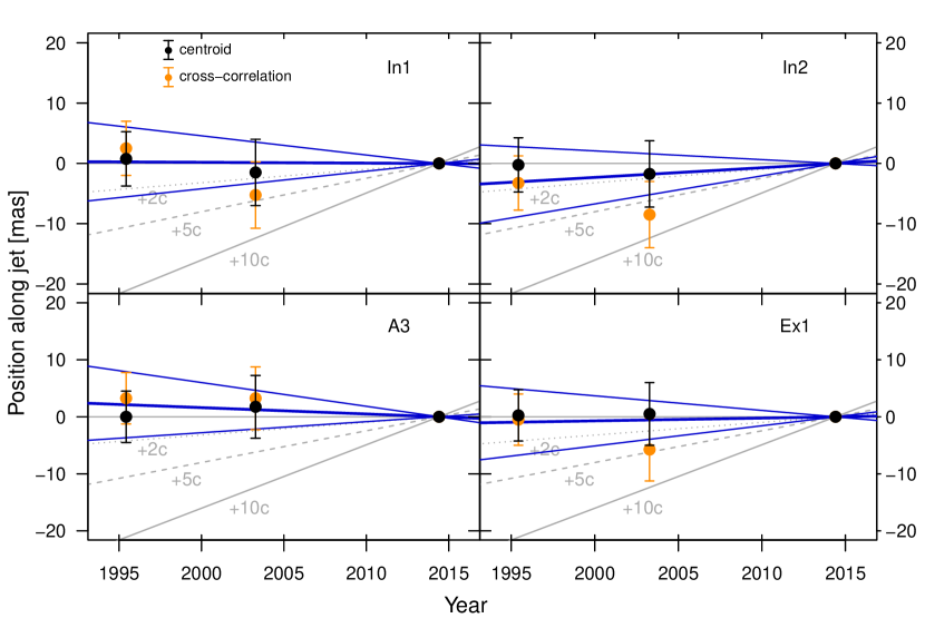
Figure 6.— Shift of 4 nearby galaxies to the jet (name noted at upper right of each panel) versus time relative to the 2014 measured position. Black points represent the contour-derived shifts and orange points the cross-correlation derived shifts. As a guide, lines corresponding to an apparent forward speed of 2$c$ (dotted gray) and 5$c$ (dashed gray) and 10$c$ (solid gray) are plotted in each subfigure. The thick solid blue line is the best-fit weighted linear regression model to all points, while the thinner blue lines show the 2$\sigma$ (95%) upper and lower limit slopes.

Table 2 Positions Relative to 2014 (Parallel and Transverse to Jet Axis)

	Contour Method					Cross-Correlation Method
Name	Rap	$\delta x_{\mathrm{1995}}$	$\delta y_{\mathrm{1995}}$	$\delta x_{\mathrm{2003}}$	$\delta y_{\mathrm{2003}}$	$\delta x_{\mathrm{1995}}$	$\delta y_{\mathrm{1995}}$	$\delta x_{\mathrm{2003}}$	$\delta y_{\mathrm{2003}}$
(1)	(2)	(3)	(4)	(5)	(6)	(7)	(8)	(9)	(10)
A1		$-$0.16$\pm$ 0.19	$-$0.07$\pm$ 0.19	$-$0.04$\pm$ 0.23	$-$0.18$\pm$ 0.22	$-$0.21$\pm$ 0.18	$-$0.04$\pm$ 0.18	$-$0.03$\pm$ 0.22	$-$0.04$\pm$ 0.22
A2	10	$-$0.07$\pm$ 0.18	$-$0.07$\pm$ 0.18	$-$0.02$\pm$ 0.22	$-$0.03$\pm$ 0.22	$-$0.41$\pm$ 0.18	$-$0.26$\pm$ 0.18	$-$0.04$\pm$ 0.22	$-$0.08$\pm$ 0.22
B1		$-$0.27$\pm$ 0.20	$-$0.20$\pm$ 0.20	$-$0.18$\pm$ 0.23	$-$0.07$\pm$ 0.23	$-$0.31$\pm$ 0.18	$-$0.11$\pm$ 0.18	$-$0.22$\pm$ 0.22	$-$0.09$\pm$ 0.22
B2	6.2	$-$0.04$\pm$ 0.18	$-$0.04$\pm$ 0.18	$-$0.08$\pm$ 0.22	$-$0.05$\pm$ 0.22	$-$0.18$\pm$ 0.18	$-$0.10$\pm$ 0.18	$-$0.48$\pm$ 0.22	$-$0.37$\pm$ 0.22
C1	8.2	$-$0.04$\pm$ 0.18	$-$0.00$\pm$ 0.18	$-$0.08$\pm$ 0.22	$-$0.00$\pm$ 0.22	$-$0.01$\pm$ 0.18	$-$0.02$\pm$ 0.18	$-$0.49$\pm$ 0.22	$-$0.04$\pm$ 0.22
C2	7	$-$0.01$\pm$ 0.18	$-$0.00$\pm$ 0.18	$-$0.02$\pm$ 0.22	$-$0.01$\pm$ 0.22	$-$0.20$\pm$ 0.18	$-$0.07$\pm$ 0.18	$-$0.25$\pm$ 0.22	$-$0.03$\pm$ 0.22
C3	7	$-$0.06$\pm$ 0.18	$-$0.00$\pm$ 0.18	$-$0.04$\pm$ 0.22	$-$0.07$\pm$ 0.22	$-$0.01$\pm$ 0.18	$-$0.08$\pm$ 0.18	$-$0.15$\pm$ 0.22	$-$0.03$\pm$ 0.22
D		$-$0.14$\pm$ 0.19	$-$0.23$\pm$ 0.19	$-$0.15$\pm$ 0.23	$-$0.02$\pm$ 0.23	$-$0.03$\pm$ 0.18	$-$0.18$\pm$ 0.18	$-$0.02$\pm$ 0.22	$-$0.18$\pm$ 0.22
H2	5	$-$0.01$\pm$ 0.18	$-$0.01$\pm$ 0.18	$-$0.04$\pm$ 0.22	$-$0.09$\pm$ 0.22	$-$0.08$\pm$ 0.18	$-$0.05$\pm$ 0.18	$-$0.05$\pm$ 0.22	$-$0.29$\pm$ 0.22
H3		$-$0.13$\pm$ 0.19	$-$0.01$\pm$ 0.19	$-$0.17$\pm$ 0.26	$-$0.38$\pm$ 0.26	$-$0.05$\pm$ 0.18	$-$0.13$\pm$ 0.18	$-$0.06$\pm$ 0.22	$-$0.00$\pm$ 0.22

Table 3 Proper Motion Measurements for 3C 273 and Field Sources

Name	Flux	Aperture	SB	$\mu_{app,X}$	$\mu_{app,Y}$	$\beta_{app,X}$	$\beta_{app,Y}$	P($\beta_{app,X}$)$>0$	99% UL $\beta_{app,X}$
	($\mu$Jy)	(pixels)	$\mu$Jy/′′2	(mas yr-1)	(mas yr-1)
A1	3.7	51x20	24.8	$-$0.19$\pm$0.16	$-$0.09$\pm$0.16	$-$1.7$\pm$1.4	$-$0.8$\pm$1.4	$>$12%	1.6
A2	1.2	12.7	6.7	$-$0.07$\pm$0.22	$-$0.09$\pm$0.22	$-$0.6$\pm$1.9	$-$0.8$\pm$1.9	$>$38%	3.8
B1	2.5	14.6	17.2	$-$0.22$\pm$0.16	$-$0.19$\pm$0.16	$-$2.0$\pm$1.4	$-$1.7$\pm$1.4	$>$ 8%	1.3
B2	1.0	9	9.0	$-$0.01$\pm$0.22	$-$0.06$\pm$0.22	$-$0.1$\pm$1.9	$-$0.6$\pm$1.9	$>$48%	4.3
C1	3.0	19.8	10.7	$-$0.10$\pm$0.15	$-$0.02$\pm$0.15	$-$0.9$\pm$1.4	$-$0.2$\pm$1.4	$>$75%	4.2
C2	0.8	7.3	10.6	$-$0.06$\pm$0.15	$-$0.03$\pm$0.15	$-$0.5$\pm$1.4	$-$0.3$\pm$1.4	$>$36%	2.8
C3	1.6	10.5	10.6	$-$0.07$\pm$0.15	$-$0.03$\pm$0.15	$-$0.6$\pm$1.4	$-$0.3$\pm$1.4	$>$67%	3.9
D	1.9	10.1	17.6	$-$0.02$\pm$0.16	$-$0.26$\pm$0.16	$-$0.2$\pm$1.4	$-$2.4$\pm$1.4	$>$55%	3.5
H3	4.3	22x44	18.0	$-$0.02$\pm$0.16	$-$0.14$\pm$0.16	$-$0.2$\pm$1.4	$-$1.3$\pm$1.4	$>$56%	3.5
H2	0.5	8.7	6.1	$-$0.07$\pm$0.15	$-$0.11$\pm$0.15	$-$0.6$\pm$1.4	$-$1.0$\pm$1.4	$>$67%	3.9
In1*	0.0		0.0	$-$0.01$\pm$0.15	$-$0.06$\pm$0.15	$-$0.1$\pm$1.4	$-$0.6$\pm$1.4	$>$46%	3.2
In2*	0.0		0.0	$-$0.16$\pm$0.15	$-$0.02$\pm$0.15	$-$1.4$\pm$1.4	$-$0.1$\pm$1.4	$>$85%	4.7
A3*	0.0		0.0	$-$0.11$\pm$0.15	$-$0.27$\pm$0.15	$-$1.0$\pm$1.4	$-$2.4$\pm$1.4	$>$23%	2.3
Ex1*	0.0		0.0	$-$0.05$\pm$0.15	$-$0.06$\pm$0.15	$-$0.4$\pm$1.4	$-$0.5$\pm$1.4	$>$63%	3.7
fs	0.0		0.0	$-$1.79$\pm$0.39	$-$0.65$\pm$0.37	$-$16.1$\pm$3.5	$-$5.8$\pm$3.3	$>$100%	24.3

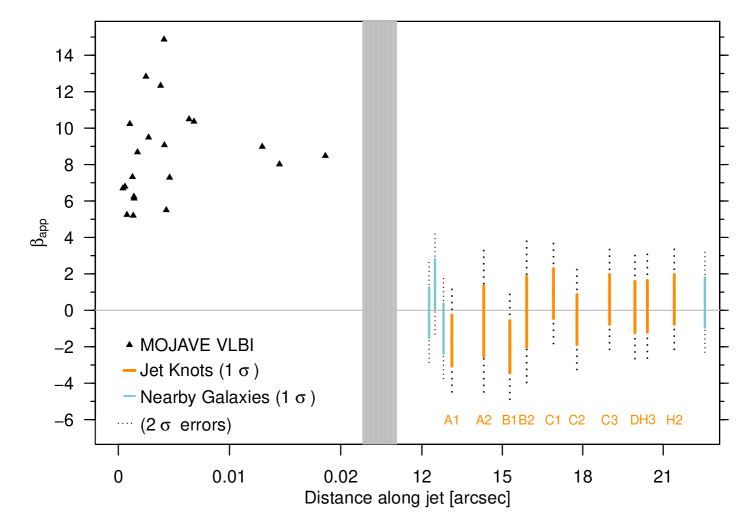
Figure 7.— A comparison of jet speeds with distance in the 3C 273 jet. The radio VLBI-measured jet speeds for the sub-arcsecond scale jet from Lister et al. (2013) are shown as black triangles (note that the error bars are smaller than the symbol size). The distance scale is broken at the gray bar to allow the near-and-far velocity fields to be compared. Our data for the kpc-scale jet of 3C 273 is shown as orange lines spanning the 1$\sigma$ error range, with dotted black lines giving the 2$\sigma$ error range. The blue lines and dotted extensions give the 1$\sigma$ and 2$\sigma$ measurements for the four background galaxies labeled in Figure 1.

4. Discussion

4.1. The velocity of the knots in the kpc-scale Jet

As shown in Table 3, we do not detect significant proper motions in any of the knots in the jet of 3C 273. Only for the bright knots A1 and A2 is there a slight case for a significant negative proper motion, just above the 1$\sigma$ level, but we do not claim this as a robust detection. These knots, like all other knots, do not show any significant flux change over the 20 year timespan of the study, and an examination of the isophotes used in the contour method of position measurement did not suggest that any major change in knot shape (such as an increased north-west extension of the knot) could be responsible for the observed negative value. As shown in column 9 of Table 3, none of the knots has a probability of speed greater than zero which rises to the level of significance (i.e, $>$95%). In general, the lack of knot proper-motion detections is not due to lack of proper-motions sensitivity in our study: if the knots in 3C273 had motions on the order of 5-7$c$ (corresponding to 0.56$-$0.78 mas yr^-1), as found previously in M87 and 3C264, we would have been able to detect these motions. The sensitivity of the study is also demonstrated by the significant proper motion measured for the foreground star (‘fs’ in Table 3).

We show in Figure 7 a comparison of our kpc-scale proper motion measurements with the parsec-scale jet speeds probed by radio interferometry by the MOJAVE project (Lister et al., 2013). The independent axis is distance measured from the core along the jet direction. The black triangles are the VLBI jet speeds (error bars are less than the symbol size), which reach values up to 15$c$. Our results for the kpc-scale knots are shown as orange lines, spanning 1$\sigma$ errors, with dotted-black-line extensions representing the 2$\sigma$ error range. The distance scale is linear but with a break to show the two datasets side-by-side. We also show for comparison in blue our measurements for the four nearby galaxies labeled in Figure 1. These data points counter the slight impression that there is a bias towards more positive values of the proper motions with increasing distance along the jet, ruling out that this is due to any systematic bias in the image registration. Indeed, the range of speeds observed for the background galaxies, known to have a proper motion of absolutely zero, suggests that the spread in knot speeds is due to the random measurement error.

The VLBI speed data suggest the possibility of a deceleration with distance already starting on parsec-scales, as shown in Figure 7. If the three most distant points measured by VLBI accurately represent the maximum speed compared to the highest upstream speed of nearly 15$c$, both exponential and linear fits suggest the jet will reach mildly relativistic speeds ($\beta_{app}\approx 1$) within an arcsecond (2.6 kpc, projected) of the core, well before the distance to the optical jet which begins $\approx$12^′′ further on from the core. A similar result is seen in M87, where the maximum speed reached at HST-1 of 6$c$ drops to speeds of $<$2$c$ within a kpc (Biretta et al., 1999; Meyer et al., 2013). Indeed, it should be emphasized that while we refer to the jets of M87, 3C 264, and 3C 273 as “kpc-scale”, the jet of 3C 273, at $\approx$200-400 kpc (deprojected) is likely 40-100 times longer than the lower-power FR I sources. A recent acceleration study by the MOJAVE program (Homan et al., 2015) shows that some sources switch from acceleration to deceleration beyond sub-kpc scales. It may simply be that even though 3C 273 starts out with a much higher speed, the distance to knot A is such that the jet has slowed down appreciably. It is also worth noting that 3C 273 is somewhat unusual in not having hotspots, which are usually interpreted as the point of final deceleration of a powerful, still-relativistic jet, which may also indicate that the jet has slowed either before or at the optical jet.

4.2. Constraints on the Physical Conditions in the kpc-scale Knots

We now discuss the limits the present and previous observations yield for two important physical parameters: the real speed $\beta$ and the angle to the line-of-sight $\theta$ (Figure 8). Understanding the allowed parameter space will in turn allow us to evaluate the energetic requirements and fitness of different physical models for the kpc-scale knots. Two possible scenarios are before us: either the knots are moving packets of plasma, or these features represent ‘standing shock’ features which move much more slowly than the bulk plasma speed.

The maximum observed speed of 15$c$ measured by the MOJAVE project implies an angle no larger than 7.6^∘ as an absolute maximum (assuming $\beta=1$) or 7.2^∘ to the line-of-sight for the parsec-scale jet if we assume that $\Gamma<50$ as implied by the maximum speeds observed for the entire sample of VLBI-observed jets (e.g., Lister et al., 2009). No deviations are seen from parsec to kpc scales in 3C 273 which would suggest any bending in or out of the line-of-sight. We therefore adopt the 7.2^∘ as the maximum angle for the kpc-scale jet as well. A further global limit on the angle to the line-of-sight can be calculated by assuming that the 24^′′ jet does not exceed 1 Mpc in total (deprojected) length, as very few radio galaxies exceed this length (e.g. 3C 236, Schilizzi et al., 2001); this gives a lower limit $\theta=3.8^{\circ}$. These minimum and maximum angles are plotted as horizontal lines in Figure 8.

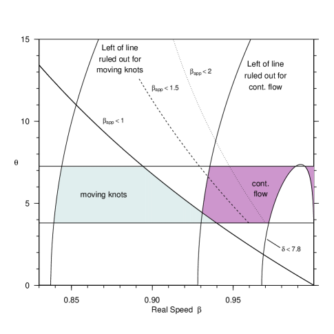
Figure 8.— This plot shows the allowed range of real jet speed $\beta$ and the angle to the line-of-sight $\theta$ under two possible scenarios. The light-blue shaded area corresponds to the allowed region if the optical knots are moving components, while the mauve region corresponds to the allowed parameters if the optical jet is a continuous flow (and the knots are shock features). For both areas, the left boundary is formed by the curves dictated by the jet-to-counterjet ratio $R>10^{4}$ in each case (Conway et al. 1993, see also Georganopoulos et al. 2006), and the entire jet is subject to the limits on viewing angle of 3.8${}^{\circ}<\theta<$7.2^∘ dictated by the condition that the jet not exceed 1 Mpc in length or a $\Gamma>50$ in the parsec-scale jet (see text). For the moving knots case, the thick upper-right boundary corresponds to the limit from our observations that $\beta_{app}<1c$ for knot A1. In the continuous flow case, there is an additional boundary from the condition that $\delta<$7.8 from Meyer et al. (2015a). Within the allowed ‘moving knots’ region, the maximum speed $\beta=0.94$, which corresponds to a limit $\Gamma\leqslant 2.9$ and $\delta\leqslant 5.5$ at this point.

If we assume that the optical knots are ‘ballistic’ packets of moving plasma, a limit of $\beta_{\mathrm{app}}<1c$ on the knot speeds can be used to derive a limit in the $\beta-\theta$ plane, as shown in Figure 8 as the slanting black line bounding the right of the allowed zone under the moving knots scenario (more conservative limits of 1.5$c$ and 2$c$ are shown as dashed and dotted lines as labeled). Further, the observation that the jet-to-counterjet ratio $R$ exceeds 10⁴ (Conway et al., 1993) leads to the left boundary to this area, where R=(1+$\beta$cos$\theta$)^m+α/(1-$\beta$cos$\theta$)^m+α. In the case of moving knots $m=3$ and for a continous flow $m=2$, while we take $\alpha$=0.8 from radio observations (see Georganopoulos et al., 2006). The jet-to-counterjet ratio limit thus also leads to a left bound on the allowed area for a continuous flow jet, as shown in Figure 8. Note that the two zones (moving knots versus continuous flow) are nearly mutually exclusive only under the $\beta_{\mathrm{app}}<1c$ limit. Under the more conservative (larger) upper limits for $\beta_{\mathrm{app}}$, the moving knots allowed zone extends to higher $\beta$ values, overlapping with purple-shaded the continuous flow region.

The allowed range of $\beta$ according to the boundaries in Figure 8 in the moving knots case under $\beta_{\mathrm{app}}<1c$ is 0.84$<\beta<0.94$, corresponding to 1.8$<\Gamma<2.9$. The maximum $\Gamma$ increases to 3.6 for a limit $1.5c$ and $4.1$ for a limit of $2c$. The maximum Doppler beaming factor in the allowed zone under any of the $\beta_{\mathrm{app}}$ limits is found at the point of minimum angle (3.8^∘) and maximum jet speed. For $\beta_{\mathrm{app}}<1c$, $1.5c$, and $2c$, respectively, the upper limit on $\delta$ is 5.5, 6.7, and 7.6. As we discuss below, these $\delta$ values are considerably lower than the $\delta=20$ required (under equipartition) in the large-scale jet if the X-ray emission from the knots is from the IC/CMB process.

4.3. Implications for the IC/CMB Model for the X-ray emission

The kpc-scale jet of 3C 273 has been detected by Chandra in the X-rays (Marshall et al., 2001; Jester et al., 2006), where the hard spectrum and high flux level of the knots shows that the X-rays are due to a separate component from the radio-optical synchrotron spectrum. Indeed, HST observations by Jester et al. (2007) show that the spectrum is already upturning into this second component at UV energies. The jet of 3C 273 is one of dozens of ‘anomalous’ X-ray jets discovered by Chandra to have hard and high X-ray fluxes in the knots which require a second component (e.g., Harris & Krawczynski, 2006, for a review). The most favored explanation for the X-rays in these jets has been that the large-scale jet remains as highly relativistic as the parsec-scale jet, with $\Gamma$$\approx$10 or more. Coupled with a small angle to the line-of-sight, the increased Doppler boosting suggests that the X-rays could be consistent with inverse Compton upscattering of CMB photons by the same electron population that produces the radio-optical synchrotron spectrum, assuming the electron energy distribution can be extended to much lower energies than traced by GHz radio observations (Tavecchio et al., 2000; Celotti et al., 2001; Jester et al., 2006). Alternatively, it has been suggested that the second component producing the X-rays could be synchrotron in origin, from a separate electron energy distribution which reaches multi-TeV energies (Harris et al., 2004; Kataoka & Stawarz, 2005; Hardcastle, 2006; Jester et al., 2006; Uchiyama et al., 2006). The differences between the IC/CMB and synchrotron mechanisms are important: the former requires a fast and powerful jet (sometimes near or super-Eddington), while the latter suggests a slower and less powerful jet on kpc scales (Georganopoulos et al., 2006). The main opposition to the synchrotron interpretation remains its unclear origin (Atoyan & Dermer, 2002; Aharonian, 2002; Liu et al., 2015).

While IC/CMB is a popular explanation for anomalous X-ray jets, it has now been ruled out explicitly in three cases: for PKS 1136-135 based on UV polarization in the second spectral component (Cara et al., 2013), and for PKS 0637-752 and 3C 273 based on non-detection of the gamma-rays implied by the IC/CMB model (Meyer & Georganopoulos, 2014; Meyer et al., 2015a), an idea first proposed by Georganopoulos et al. (2006). In the case of 3C 273, we show here in an independent way that the IC/CMB model is also disfavored by our proper motions upper limits.

It has already been shown that the X-rays from the knots of 3C 273 and similar jets, can only be compatible with an IC/CMB origin if the knots are moving packets. This is because in the case of particle-accelerating standing shocks in the IC/CMB model, the extremely long (hundreds of Mpc) cooling length of the low energy X-ray emitting electrons would result in continuously-emitting X-ray jets, instead of the observed knotty appearance (Atoyan & Dermer, 2002). This is avoided in the case of a moving packet of plasma, as the low energy electrons remain confined within the packet.

The minimum power configuration for the first and brightest knot A1 is that of equipartition between radiating electron and magnetic field energy density. With the additional assumption that the Lorentz factor equals the Doppler factor, $\Gamma=\delta$ , this requires $\delta=20$. All configurations, however, with $\delta>7.6$ are excluded because of the constraints discussed above. This requires that we move away from the equipartition power requirement of $10^{48}$ erg s^-1 (assuming one proton per radiating electron), to $5\times 10^{48}$ erg s^-1 for the minimum power configuration in the permitted zone at the extreme edge where $\theta=3.8^{\circ}$, $\delta=5.5$. Elsewhere in the allowed moving-knots zone the minimum power is even higher.

We compare now this power to the Eddington luminosity of the source. Mass estimates for the black hole of 3C 273 vary widely, from $2\times 10^{7}\,M_{\odot}$ (Wang et al., 2004) to $4\times 10^{8}\,M_{\odot}$ (Pian et al., 2005) to $6.6\times 10^{9}\,M_{\odot}$ (Paltani & Türler, 2005). Even for the highest mass estimate, the Eddington luminosity is $10^{48}$ erg s^-1. This is barely compatible with the equipartition configuration, which however we disfavor because it does not comply with our angle and superluminal motion constraints. The minimum jet power compatible with $\delta<5.5$ is five times higher than the Eddington luminosity, adopting the highest black hole mass for 3C 273. Given that the jet power is in general found to be sub-Eddington (Ghisellini et al., 2014) we disfavor the IC/CMB mechanism for the production of the X-rays, as it requires a power of at least five times Eddington, and up to several hundred times Eddington depending on the black hole mass.

5. Conclusions

We have used new and archival HST V-band imaging of the optical jet in 3C 273 to look for significant proper motions of the major knots over the 19 years between June 1995 and May of 2014. We have described a method of image registration based on background galaxies; in the 2014 deep ACS imaging, our systematic error in the stacking is 0.44 mas, while the systematic error of registration for the 1995 and 2003 epochs of WFPC2/PC imaging is 4.5 and 2.8 mas, respectively. We have used both a two-dimensional cross-correlation and a centroiding technique to measure relative shifts in the knots both along and perpendicular to the jet direction. Our results show that all knots have speeds consistent with zero with typical 1$\sigma$ errors on the order of 0.1$-$0.2 mas/year or 1.5$c$, and with 99% upper limit values ranging from $1-5$c. We have used nearby background galaxies to show that these limits are consistent with stationary objects in the same field.

These results suggest that the knots in the kpc-scale jet, if they are moving packets of plasma, must be relatively slow, in agreement with previous studies based on jet-to-counterjet ratios in radio-loud populations (Arshakian & Longair, 2004; Mullin & Hardcastle, 2009). Assuming that the jet either remains at the same speed or decelerates as you move downstream, the $2\sigma$ upper limit speed derived from all knots combined of $1c$ suggests that the entire optical jet is at most mildly relativistic, with a maximum Lorentz factor of $\Gamma<2.9$. However, we cannot rule out the possibility that the knots are standing shock features in the flow, where the bulk plasma moves through the features with a higher $\Gamma$. The best limits on the bulk plasma speed thus remain the limits derived from the non-detection of the IC/CMB component in gamma-rays by Meyer et al. (2015a), where $\delta<7.8$ is implied assuming equipartition magnetic fields.

Finally, we show that the observed upper limits on the proper motion of the knots confirms that the a near-equipartition IC/CMB model for the X-rays of the kpc-scale knots is ruled out. The equipartition IC/CMB model requires that the knots are ballistic packets of moving plasma moving at the bulk speed $\Gamma\approx 15-20$ which would imply proper motions on the order of 10$c$ or 1.12 mas/year which could have been detected in our study; our upper limits easily rule this out at a high level of significance ($>$5$\sigma$). Moving away from equipartition conditions, an IC/CMB model consistent with our observations requires a jet power on the order of five to several hundred times the Eddington limit, and is thus energetically disfavored.

In comparison to other recent HST observations of lower-power optical jets M87 and 3C264, where highly superluminal speeds (6$-$7$c$) have been observed in the optical kpc-scale jet, our first proper-motion study of a powerful quasar jet reveals no significant proper motions. It remains to be seen whether this is because the jet has truly decelerated and is only mildly relativistic, or because the knot features in sources like M87 and 3C 273 represent very different things: moving packets of plasma in the first instance and standing shocks in the second.

Appendix A CTE Correction Maps

Losses due to charge transfer inefficiency (CTI=1-CTE) in the WFPC2 detectors is fairly well-studied problem. The first correction formulae were published by (Whitmore et al., 1999, hereafter WHC99), and later updated by Dolphin (2000), in both cases based on observations of stars. A comparison between the two shows reasonably good agreement (Whitmore & Heyer, 2002), with the WHC99 formulae producing smaller corrections at very low flux levels. We have used the WHC99 formulae in our corrections, but the method of producing pixel-by-pixel maps presented here could be used with any set of corrections.

Applying the WHC99 CTE loss correction formulae directly to the measured fluxes for the jet or galaxies in our imaging would be inappropriate because they are resolved, while the formulae are based on fixed-aperture observations of stars. We also wished to produce CTE-corrected frames from the pipeline-produced ‘c0f’ files to use in registering the images through the background galaxies, where accurate flux levels are obviously helpful. Therefore, a pixel-by-pixel correction ‘map’ for each raw image is needed. Note that this method is not flux-conserving, but seems to work well in recovering the total flux in bright, resolved, but relatively compact sources such as the jet knots and background galaxies.

To produce these maps, we first measured the background level in each raw image – usually about 8 counts/pixel in 1995 and 3 counts/pixel in 2003. In order to calculate the corrected flux in each pixel, we need the modified Julian date (MJD) of the observation, the $x$ and $y$ location on the detector, the background flux level, the ‘source’ flux (total - background) and the WHC99 formulae. We have assumed that the CTE corrections have the same form (though not the same parameters) when based on the pixel value as when based on the total flux of a star within a radius=2 pixel aperture. We transformed between these representations of the correction by using a ‘known’ PSF, generated by the tinytim package, for the F622W filter using a powerlaw form and otherwise standard parameters. Since the original correction formulae were based on a 2-pixel-radius aperture, we only need the PSF to be defined within an aperture of this size.

The correction at each pixel $i$ is assumed to have the form:

$$x_{cts,i}=\left(\alpha_{x}+\beta_{x}\log\left(\mathrm{cts}_{0,i}\right)\right)\mathrm{cts}_{0,i}$$ (A1)

$$y_{cts,i}=\left(\alpha_{y}+\beta_{y}\log\left(\mathrm{cts}_{0,i}\right)\right)\mathrm{cts}_{0,i}$$ (A2)

where the counts in the pixel before CTE losses is cts_0,i and $x_{cts,i}$ and $y_{cts,i}$ are the corrections for CTE losses in the x and y directions, respectively, in DN. We want to determine the values of the $\alpha$ and $\beta$ parameters individually for each pixel.

To do that, we choose a vector of simulated observed stars with counts before CTE losses of $T^{*}_{0}$, and measured counts $T^{*}_{M}$ in the two-pixel radius aperture. Starting with a vector of $T^{*}_{M}$ values, the WHC99 formulae and properties of the pixel and image are used to get the values of $T^{*}_{0}$, $x_{cts}$ and $y_{cts}$, noting that $T^{*}_{0}=x_{cts}+y_{cts}+T^{*}_{M}$. These vectors can be related to the individual pixels falling within the aperture in the following way:

$$y_{cts}=\sum_{i}y_{cts,i}f_{i}$$ (A3)

where $y_{cts}$ is the total correction due to y-direction CTE losses for all the pixels within the aperture. Because we have used a circular aperture, the fraction $f_{i}$ is used to only count the portion of the pixel that falls within the two-pixel radius, which we have assumed is centered on the PSF. A similar equation holds in the x-direction. The vectors based on ‘stars’ can be used to derive the $\alpha$/$\beta$ parameters from the following linear relation:

$$\frac{y_{cts}}{S_{1}}=\alpha_{y}+\beta_{y}\frac{S_{2}}{S_{1}}$$ (A4)

where

$$S_{1}=\sum_{i}\mathrm{cts}_{0,i}f_{i}=T^{*}_{0}\sum_{i}c_{i}f_{i}=T^{*}_{0}$$ (A5)

$$S_{2}=\sum_{i}\mathrm{cts}_{0,i}\log\left(\mathrm{cts}_{0,i}\right)f_{i}=T^{*}_{0}\sum_{i}c_{i}f_{i}\log\left(T^{*}_{0}\mathrm{cts}_{0,i}\right)$$ (A6)

Note that the quantities $c_{i}$ define the PSF inside the aperture such that

$$\sum_{i}c_{i}f_{i}=1.$$ (A7)

Using values of $T_{M}$ around the value of the observed pixel counts, a linear least-squares fitting can easily derive the values of $\alpha_{y}$ and $\beta_{y}$ for equation A4, and similarly for $\alpha_{x}$ and $\beta_{x}$. These then become the parameters for calculating the pixel-based, rather than aperture-based correction.

References

- Agudo et al. (2012) Agudo, I., Gómez, J. L., Casadio, C., Cawthorne, T. V., & Roca-Sogorb, M. 2012, ApJ, 752, 92
- Aharonian (2002) Aharonian, F. A. 2002, MNRAS, 332, 215
- Alberdi et al. (2000) Alberdi, A., Gómez, J. L., Marcaide, J. M., Marscher, A. P., & Pérez-Torres, M. A. 2000, A&A, 361, 529
- Arshakian & Longair (2004) Arshakian, T. G., & Longair, M. S. 2004, MNRAS, 351, 727
- Atoyan & Dermer (2002) Atoyan, A., & Dermer, C. 2002, in APS Meeting Abstracts, 11003
- Bahcall et al. (1995) Bahcall, J. N., Kirhakos, S., Schneider, D. P., et al. 1995, ApJ, 452, L91
- Biretta et al. (1999) Biretta, J. A., Sparks, W. B., & Macchetto, F. 1999, ApJ, 520, 621
- Biretta et al. (1995) Biretta, J. A., Zhou, F., & Owen, F. N. 1995, ApJ, 447, 582
- Cara et al. (2013) Cara, M., Perlman, E. S., Uchiyama, Y., et al. 2013, ApJ, 773, 186
- Celotti et al. (2001) Celotti, A., Ghisellini, G., & Chiaberge, M. 2001, MNRAS, 321, L1
- Cheung et al. (2007) Cheung, C. C., Harris, D. E., & Stawarz, Ł. 2007, ApJ, 663, L65
- Conway et al. (1981) Conway, R. G., Davis, R. J., Foley, A. R., & Ray, T. P. 1981, Nature, 294, 540
- Conway et al. (1993) Conway, R. G., Garrington, S. T., Perley, R. A., & Biretta, J. A. 1993, A&A, 267, 347
- Deason et al. (2013) Deason, A. J., Van der Marel, R. P., Guhathakurta, P., Sohn, S. T., & Brown, T. M. 2013, ApJ, 766, 24
- Dolphin (2000) Dolphin, A. E. 2000, PASP, 112, 1397
- Fabian (2012) Fabian, A. C. 2012, ARA&A, 50, 455
- Georganopoulos et al. (2006) Georganopoulos, M., Perlman, E. S., Kazanas, D., & McEnery, J. 2006, ApJ, 653, L5
- Ghisellini et al. (2014) Ghisellini, G., Tavecchio, F., Maraschi, L., Celotti, A., & Sbarrato, T. 2014, Nature, 515, 376
- Giovannini et al. (2001) Giovannini, G., Cotton, W. D., Feretti, L., Lara, L., & Venturi, T. 2001, ApJ, 552, 508
- Hardcastle (2006) Hardcastle, M. J. 2006, MNRAS, 366, 1465
- Harris & Krawczynski (2006) Harris, D. E., & Krawczynski, H. 2006, ARA&A, 44, 463
- Harris et al. (2004) Harris, D. E., Mossman, A. E., & Walker, R. C. 2004, ApJ, 615, 161
- Harris & Stern (1987) Harris, D. E., & Stern, C. P. 1987, ApJ, 313, 136
- Homan et al. (2015) Homan, D. C., Lister, M. L., Kovalev, Y. Y., et al. 2015, ApJ, 798, 134
- Jester et al. (2006) Jester, S., Harris, D. E., Marshall, H. L., & Meisenheimer, K. 2006, ApJ, 648, 900
- Jester et al. (2007) Jester, S., Meisenheimer, K., Martel, A. R., Perlman, E. S., & Sparks, W. B. 2007, MNRAS, 380, 828
- Jester et al. (2005) Jester, S., Röser, H.-J., Meisenheimer, K., & Perley, R. 2005, A&A, 431, 477
- Jester et al. (2001) Jester, S., Röser, H.-J., Meisenheimer, K., Perley, R., & Conway, R. 2001, A&A, 373, 447
- Jorstad et al. (2001) Jorstad, S. G., Marscher, A. P., Mattox, J. R., et al. 2001, ApJS, 134, 181
- Jorstad et al. (2005) Jorstad, S. G., Marscher, A. P., Lister, M. L., et al. 2005, AJ, 130, 1418
- Kataoka & Stawarz (2005) Kataoka, J., & Stawarz, Ł. 2005, ApJ, 622, 797
- Kellermann et al. (1999) Kellermann, K. I., Vermeulen, R. C., Zensus, J. A., Cohen, M. H., & West, A. 1999, New A Rev., 43, 757
- Kellermann et al. (2004) Kellermann, K. I., Lister, M. L., Homan, D. C., et al. 2004, ApJ, 609, 539
- Lelievre et al. (1984) Lelievre, G., Nieto, J.-L., Horville, D., Renard, L., & Servan, B. 1984, A&A, 138, 49
- Lister et al. (2009) Lister, M. L., Cohen, M. H., Homan, D. C., et al. 2009, AJ, 138, 1874
- Lister et al. (2013) Lister, M. L., Aller, M. F., Aller, H. D., et al. 2013, AJ, 146, 120
- Liu et al. (2015) Liu, W.-P., Chen, Y. J., & Wang, C.-C. 2015, ApJ, 806, 188
- Marshall et al. (2001) Marshall, H. L., Harris, D. E., Grimes, J. P., et al. 2001, ApJ, 549, L167
- Meyer & Georganopoulos (2014) Meyer, E. T., & Georganopoulos, M. 2014, ApJ, 780, L27
- Meyer et al. (2015a) Meyer, E. T., Georganopoulos, M., Sparks, W. B., et al. 2015a, ApJ, 805, 154
- Meyer et al. (2013) Meyer, E. T., Sparks, W. B., Biretta, J. A., et al. 2013, ApJ, 774, L21
- Meyer et al. (2015b) Meyer, E. T., Georganopoulos, M., Sparks, W. B., et al. 2015b, Nature, 521, 495
- Mullin & Hardcastle (2009) Mullin, L. M., & Hardcastle, M. J. 2009, MNRAS, 398, 1989
- Muxlow & Wilkinson (1991) Muxlow, T. W. B., & Wilkinson, P. N. 1991, MNRAS, 251, 54
- Paltani & Türler (2005) Paltani, S., & Türler, M. 2005, A&A, 435, 811
- Pian et al. (2005) Pian, E., Falomo, R., & Treves, A. 2005, MNRAS, 361, 919
- Piner & Edwards (2004) Piner, B. G., & Edwards, P. G. 2004, ApJ, 600, 115
- Piner et al. (2010) Piner, B. G., Pant, N., & Edwards, P. G. 2010, ApJ, 723, 1150
- Sambruna et al. (2001) Sambruna, R. M., Urry, C. M., Tavecchio, F., et al. 2001, ApJ, 549, L161
- Schilizzi et al. (2001) Schilizzi, R. T., Tian, W. W., Conway, J. E., et al. 2001, A&A, 368, 398
- Schmidt et al. (1978) Schmidt, G. D., Peterson, B. M., & Beaver, E. A. 1978, ApJ, 220, L31
- Stawarz et al. (2006) Stawarz, Ł., Aharonian, F., Kataoka, J., et al. 2006, MNRAS, 370, 981
- Tavecchio et al. (2000) Tavecchio, F., Maraschi, L., Sambruna, R. M., & Urry, C. M. 2000, ApJ, 544, L23
- Thomson et al. (1993) Thomson, R. C., Mackay, C. D., & Wright, A. E. 1993, Nature, 365, 133
- Tyson et al. (1982) Tyson, J. A., Baum, W. A., & Kreidl, T. 1982, ApJ, 257, L1
- Uchiyama et al. (2006) Uchiyama, Y., Urry, C. M., Cheung, C. C., et al. 2006, ApJ, 648, 910
- Walker (1997) Walker, R. C. 1997, ApJ, 488, 675
- Walker et al. (1988) Walker, R. C., Walker, M. A., & Benson, J. M. 1988, ApJ, 335, 668
- Wang et al. (2004) Wang, J.-M., Luo, B., & Ho, L. C. 2004, ApJ, 615, L9
- Whitmore & Heyer (2002) Whitmore, B., & Heyer, I. 2002, Charge Transfer Efficiency for Very Faint Objects and a Reexamination of the Long-vs-Short Problem for the WFPC2, Tech. rep.
- Whitmore et al. (1999) Whitmore, B., Heyer, I., & Casertano, S. 1999, PASP, 111, 1559