Black holes from multiplets of scalar fields in 2+1- and 3+1-dimensions

Abstract

We obtain classes of black hole solutions constructed from multiplets of scalar fields in 2+1 / 3+1 dimensions. The multi-component scalars don’t undergo a symmetry breaking so that only the isotropic modulus is effective. The Lagrangian is supplemented by a self-interacting potential which plays significant role in obtaining the exact solutions. In 2+1 / 3+1 dimensions doublet / triplet of scalars is effective which enriches the available black hole spacetimes and creates useful Liouville weighted field theoretic models.

I Introduction

The absence of gravitational degrees in lower dimensions stipulates addition of physical sources in order to make strong attraction centers and black holes. The prototype example in this regard was provided by the Bañados-Teitelboim-Zanelli (BTZ) black hole in $2+1-$dimensions which was sourced by a cosmological constant 1 ; 2 . Addition of different sources to make alternative black holes to the BTZ has always been challenging 3 ; 4 ; 5 . From this token recently we considered a doublet of scalar fields constrained to lie on the unit sphere as source in $2+1-$dimensions 6 . The uniqueness condition of the scalar fields under rotation imposes an integer parameter to play role in the metric. Two distinct classes of solutions emerged: a black hole with integer valued negative Hawking temperature and a non-black hole metric with interesting topological properties. Although extension of similar properties to $3+1-$dimensional metrics remains to be seen it is of utmost importance in connection with the belief that spacetime may be ’digital’. At the quantum (Planck) level the idea is not new but at the classical, large scale it needs concrete proof to incorporate topological numbers. Beside black holes wormholes also can be considered within the similar context. In a recent work we have shown for instance that a wormhole solution can also be obtained by employing a scalar-doublet of fields as source in $2+1-$dimensions 7 . Let’s add that multiple field scalar-tensor has been studied before 8 ; 9 ; 10 ; 11 ; 12 ; 13 ; 14 ; 15 ; 16 ; 17 ; 18 ; 19 . Triplet scalar field in the context of global monopole has been studied extensively in literature 20 ; 21 ; 22 ; 23 ; 24 ; 25 ; 26 ; 27 ; 28 ; 29 . One has to keep in order that the single scalar field coupled with gravity has been studied more rigorously. As our concentration is on $2+1-$ and $3+1-$ dimensions, we only refer to 30 ; 31 in $2+1-$ and 32 ; 33 ; 34 ; 35 ; 36 ; 37 ; 38 ; 39 ; 40 in $3+1-$dimensions.

In the present study we choose firstly our source again as a doublet of scalar fields, namely $\phi^{1}\left(r,\theta\right)=\phi\left(r\right)\cos\theta$ and $\phi^{2}\left(r,\theta\right)=\phi\left(r\right)\sin\theta,$ with the modulus $\phi\left(r\right).$ Our metric is circularly symmetric so that the angular dependence washes out leaving only the radial dependent function $\phi\left(r\right).$ In addition to the kinetic term of the scalar field we choose a suitable potential term such that our system will admit a black hole solution with interesting properties. The chosen potential with $V\left(\phi\right)$ is the product of a polynomial expression with a Liouville term. The number of parameters initially is four but with the solution the number reduces to two. The potential admits a local minimum apt to define a vacuum in the assumed field theory model. Particle states can be constructed in the potential well in analogy with the energy levels of atoms. The potential has the constant term with $\phi\left(r\right)=0$, which leads to the well-known BTZ black hole. Our solution can be interpreted as a new black hole solution constructed from a simple doublet of scalar fields. Such black holes emerge with distinct properties when compared with a singlet scalar field black holes. Secondly, we undertake the similar task to construct black holes in $3+1-$dimensions whose source consists of a triplet of scalar fields. The solution in the limit of zero scalar fields naturally reduces to the Schwarzschild-de Sitter spacetime.

Organization of the paper is as follows. Section II and III are devoted to the $2+1-$dimensional field theoretic black hole solutions. Parallel considerations for $3+1-$dimensions will be analyzed in Sections IV and V. Our brief conclusion in Section VI completes the paper.

II $2+1-$dimensional field equations

Our action in $2+1-$dimensional gravity minimally coupled to a doublet of scalar field and without cosmological constant is given by ($16\pi G=c=1$)

$$S=\int d^{3}x\sqrt{-g}\left(R+\mathcal{L}_{field}\right)$$ (1)

in which

$$\mathcal{L}_{field}=-\frac{1}{2}\left(\nabla\phi^{a}\right)^{2}-V\left(\phi\right).$$ (2)

Here

$$\left(\begin{array}[]{c}\phi^{1}\\ \phi^{2}\end{array}\right)=\phi\left(r\right)\left(\begin{array}[]{c}\cos\theta\\ \sin\theta\end{array}\right)$$ (3)

is the doublet of scalar fields with modulus

$$\phi=\phi\left(r\right)=\pm\sqrt{\phi^{a}\phi^{a}}$$ (4)

and

$$V\left(\phi\right)=V_{0}\left(1+\xi_{1}\phi+\xi_{2}\phi^{2}\right)e^{-\alpha\phi}$$ (5)

is our potential ansatz with real parameters $V_{0},$ $\xi_{1},$ $\xi_{2},$ and $\alpha\in\mathbb{R}-\left\{\pm\sqrt{2}\right\}.$ Let’s add that with specific form of potential (5), $\alpha=\pm\sqrt{2}$ does not admit a solution to our field equations therefore from the outset we exclude it. The trivial solution comes with $\phi=0$ case where we have $V\left(\phi\right)=V_{0}$ which can be considered as a cosmological constant to yield the BTZ solution.

The circularly symmetric line element is chosen to be

$$ds^{2}=-A\left(r\right)dt^{2}+\frac{1}{A(r)}dr^{2}+H\left(r\right)^{2}d\theta^{2}$$ (6)

in which $A\left(r\right)$ and $H\left(r\right)$ are two functions only of $r$. The field Lagrangian density may be cast into the following explicit form

$$\mathcal{L}_{field}=-\frac{A}{2}\phi^{\prime 2}-\frac{1}{2H^{2}}\phi^{2}-V\left(\phi\right),$$ (7)

whose variation with respect to $\phi$ yields the corresponding field equation

$$\phi^{\prime\prime}+\frac{\left(AH\right)^{\prime}}{AH}\phi^{\prime}-\frac{\phi}{AH^{2}}-\frac{V^{\prime}\left(\phi\right)}{A}=0.$$ (8)

We note that a prime stands for a derivative with respect to the argument of the function. Furthermore, variation of the action with respect to $g^{\mu\nu}$ gives the Einstein’s field equations

$$G_{\mu}^{\nu}=T_{\mu}^{\nu}$$ (9)

in which the energy momentum tensor $T_{\mu}^{\nu}$ is defined as

$$T_{\mu}^{\nu}=\frac{1}{2}\left(\partial_{\mu}\phi^{a}\partial^{\nu}\phi^{a}-\frac{1}{2}\left(\nabla\phi^{a}\right)^{2}\delta_{\mu}^{\nu}\right)-\frac{1}{2}V\left(\phi\right)\delta_{\mu}^{\nu}.$$ (10)

One may find the nonzero components of $T_{\mu}^{\nu}$ given by

$$T_{t}^{t}=-\frac{1}{4}\left(A\phi^{\prime 2}+\frac{\phi^{2}}{H^{2}}\right)-\frac{1}{2}V\left(\phi\right),$$ (11)

$$T_{r}^{r}=\frac{1}{4}\left(A\phi^{\prime 2}-\frac{\phi^{2}}{H^{2}}\right)-\frac{1}{2}V\left(\phi\right)$$ (12)

and

$$T_{\theta}^{\theta}=-\frac{1}{4}\left(A\phi^{\prime 2}-\frac{\phi^{2}}{H^{2}}\right)-\frac{1}{2}V\left(\phi\right).$$ (13)

Finally the explicit form of the Einstein’s equations are given by

$$\frac{2H^{\prime\prime}A+A^{\prime}H^{\prime}}{H}+\frac{1}{2}\left(A\phi^{\prime 2}+\frac{\phi^{2}}{H^{2}}\right)+V=0,$$ (14)

$$\frac{A^{\prime}H^{\prime}}{H}-\frac{1}{2}\left(A\phi^{\prime 2}-\frac{\phi^{2}}{H^{2}}\right)+V=0$$ (15)

and

$$A^{\prime\prime}+\frac{1}{2}\left(A\phi^{\prime 2}-\frac{\phi^{2}}{H^{2}}\right)+V=0$$ (16)

which together with (8) must be solved. In short we seek for a set of functions including $A,$ $H$ and $\phi$ which satisfy the four coupled differential equations given by (8) and (14-16).

III Solution to the field equations in $2+1-$dimensions

To solve the field equations, first we combine the $tt$ and $rr$ components of the Einstein’s equations to find

$$2H^{\prime\prime}+\phi^{\prime 2}H=0.$$ (17)

Next we consider an ansatz for $H$ given by

$$H=H_{0}e^{\frac{\alpha}{2}\phi}$$ (18)

with $H_{0}$ and $\alpha$ two parameters to be found. The latter choice and (17) yield a solution for $\phi$ as

$$\phi=\frac{2\alpha}{\alpha^{2}+2}\ln\left(C_{1}r+C_{2}\right)$$ (19)

in which $C_{1}$ and $C_{2}$ are two integration constants. We note that by introducing $\bar{r}=C_{1}r+C_{2}$ one finds $d\bar{r}=C_{1}dr$ and $\phi$ rescaled. This however, does not bring new contribution to the problem. Therefore without loss of generality 41 we set $C_{1}=1$ and $C_{2}=0$ which yields

$$\phi=\frac{2\alpha}{\alpha^{2}+2}\ln r.$$ (20)

Plugging $\phi$ and $H$ into $tt$ equation we find the solution for $A\left(r\right)$ which must satisfy the other field equations too. Doing this, however, imposes that

$$\xi_{1}=\frac{\alpha^{2}-2}{\alpha},$$ (21)

$$\xi_{2}=\frac{\left(\alpha^{2}-2\right)^{2}}{\alpha^{4}},$$ (22)

$$H_{0}^{2}=\frac{\alpha^{4}}{V_{0}\left(\alpha^{2}-2\right)^{3}}.$$ (23)

From this point on we shall make the choice $H_{0}=1$ so that the constant $V_{0}$ will be expressed in terms of $\alpha$, namely

$$V_{0}=\frac{\alpha^{4}}{\left(\alpha^{2}-2\right)^{3}}.$$ (24)

Therefore, a complete set of solutions to the field equations are given by

$$H\left(r\right)=r^{\frac{\alpha^{2}}{\alpha^{2}+2}},$$ (25)

$$\phi=\frac{2\alpha}{\alpha^{2}+2}\ln r,$$ (26)

$$V\left(\phi\right)=\frac{\alpha^{4}}{\left(\alpha^{2}-2\right)^{3}}\left(1+\frac{\alpha^{2}-2}{\alpha}\phi+\frac{\left(\alpha^{2}-2\right)^{2}}{\alpha^{4}}\phi^{2}\right)e^{-\alpha\phi}$$ (27)

with the metric function

$$A\left(r\right)=C_{0}r^{\frac{2}{\alpha^{2}+2}}\\ -\frac{\alpha^{2}r^{\frac{4}{\alpha^{2}+2}}}{\alpha^{2}-2}\left(\ln^{2}r-\frac{\left(\alpha^{2}+2\right)\left(\alpha^{2}-3\right)\ln r}{\left(\alpha^{2}-2\right)}\right.\\ +\left.\frac{\left(\alpha^{2}+2\right)^{2}\left(\alpha^{4}-5\alpha^{2}+7\right)}{2\left(\alpha^{2}-2\right)^{2}}\right),$$ (28)

in which $C_{0}$ is an integration constant. The Kretschmann scalar of the solution can be written as

$$K=\omega_{1}r^{-\frac{4\alpha^{2}}{\alpha^{2}+2}}\ln^{4}r+\omega_{2}r^{-\frac{4\alpha^{2}}{\alpha^{2}+2}}\ln^{3}r+\\ \left(\omega_{3}r^{-\frac{4\alpha^{2}+2}{\alpha^{2}+2}}+\omega_{4}r^{-\frac{4\alpha^{2}}{\alpha^{2}+2}}\right)\ln^{2}r+\\ \left(\omega_{5}r^{-\frac{4\alpha^{2}+2}{\alpha^{2}+2}}+\omega_{6}r^{-\frac{4\alpha^{2}}{\alpha^{2}+2}}\right)\ln r+\\ \omega_{7}r^{-\frac{4\alpha^{2}+2}{\alpha^{2}+2}}+\omega_{8}r^{-\frac{4\alpha^{2}+4}{\alpha^{2}+2}}+\omega_{9}r^{-\frac{4\alpha^{2}}{\alpha^{2}+2}}$$ (29)

in which $\omega_{i}$ are regular functions of $\alpha$ and $C_{0}.$ As we observe here the only singular point is the origin.

The solution for the metric function admits non-asymptotically flat black hole solutions. A transformation of the form $r=\rho^{\frac{\alpha^{2}+2}{\alpha^{2}}}$ makes the line element (6) to be of the form

$$ds^{2}=-A\left(\rho\right)dt^{2}+\frac{\left(1+\frac{2}{\alpha^{2}}\right)^{2}\rho^{\frac{4}{\alpha^{2}}}}{A(\rho)}d\rho^{2}+\rho^{2}d\theta^{2}$$ (30)

in which

$$A\left(\rho\right)=C_{0}^{\frac{2}{\alpha^{2}}}\rho-\frac{\left(\alpha^{2}+2\right)^{2}}{\alpha^{2}\left(\alpha^{2}-2\right)}\rho^{\frac{4}{\alpha^{2}}}\\ \times\left(\ln^{2}\rho-\frac{\alpha^{2}\left(\alpha^{2}-3\right)}{\left(\alpha^{2}-2\right)}\ln\rho\right.\\ +\left.\frac{\alpha^{4}\left(\alpha^{4}-5\alpha^{2}+7\right)}{2\left(\alpha^{2}-2\right)^{2}}\right).$$ (31)

Moreover, the scalar field $\phi$ becomes simply

$$\phi=\frac{2}{\alpha}\ln\rho.$$ (32)

It is needless to state that the parameter $\alpha$ ($0<\alpha<\infty,\alpha^{2}\neq 2$) represents the scalar hair of the black hole.

To complete this section we find the quasi local mass of the central black hole by applying the Brown and York (BY) formalism 42 ; 43 . This technique is used for non-asymptotically flat spherically symmetric black hole solution where an ADM mass may not be defined. According to 42 ; 43 for a spherically symmetric N-dimensional spacetime

$$ds^{2}=-F\left(\rho\right)^{2}dt^{2}+\frac{d\rho^{2}}{G\left(\rho\right)^{2}}+\rho^{2}d\Omega_{N-2}^{2}$$ (33)

the quasilocal mass is defined to be

$$M_{QL}=\lim_{\rho_{B}\rightarrow\infty}\frac{N-2}{2}\rho_{B}^{N-3}F\left(\rho_{B}\right)\left(G_{ref}\left(\rho_{B}\right)-G\left(\rho_{B}\right)\right)$$ (34)

in which $G_{ref}\left(\rho_{B}\right)$ is an arbitrary non-negative reference function and $\rho_{B}$ is the radius of the spacelike hypersurface boundary which is going to be infinite. In our case ($N=3$) we have

$$F\left(\rho_{B}\right)^{2}=A\left(\rho_{B}\right)$$ (35)

$$G\left(\rho_{B}\right)^{2}=\frac{A\left(\rho_{B}\right)\rho_{B}^{-\frac{4}{\alpha^{2}}}}{\left(1+\frac{2}{\alpha^{2}}\right)^{2}}$$ (36)

and by assuming that $A\left(\rho_{B}\right)$ diverges faster than $\rho_{B}^{\frac{2}{\alpha^{2}}}$ one finds

$$M_{QL}=-\frac{C_{0}}{4\left(1+\frac{2}{\alpha^{2}}\right)}.$$ (37)

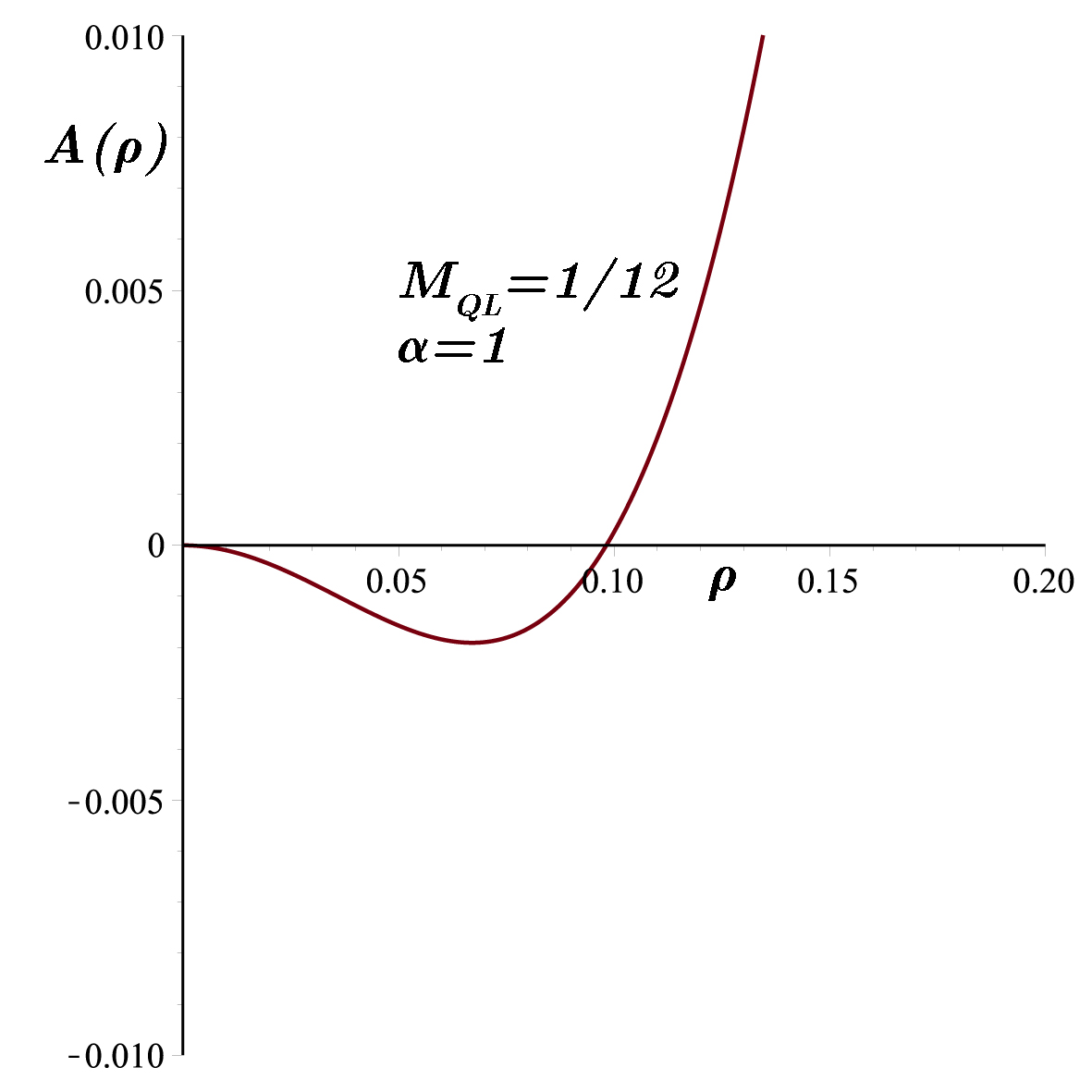
Figure 1: Metric $A\left(\rho\right)$ function versus $\rho$ for $M_{QL}=\frac{1}{12}$ and $\alpha=1$. The black hole is not asymptotically flat (Eq. 43).

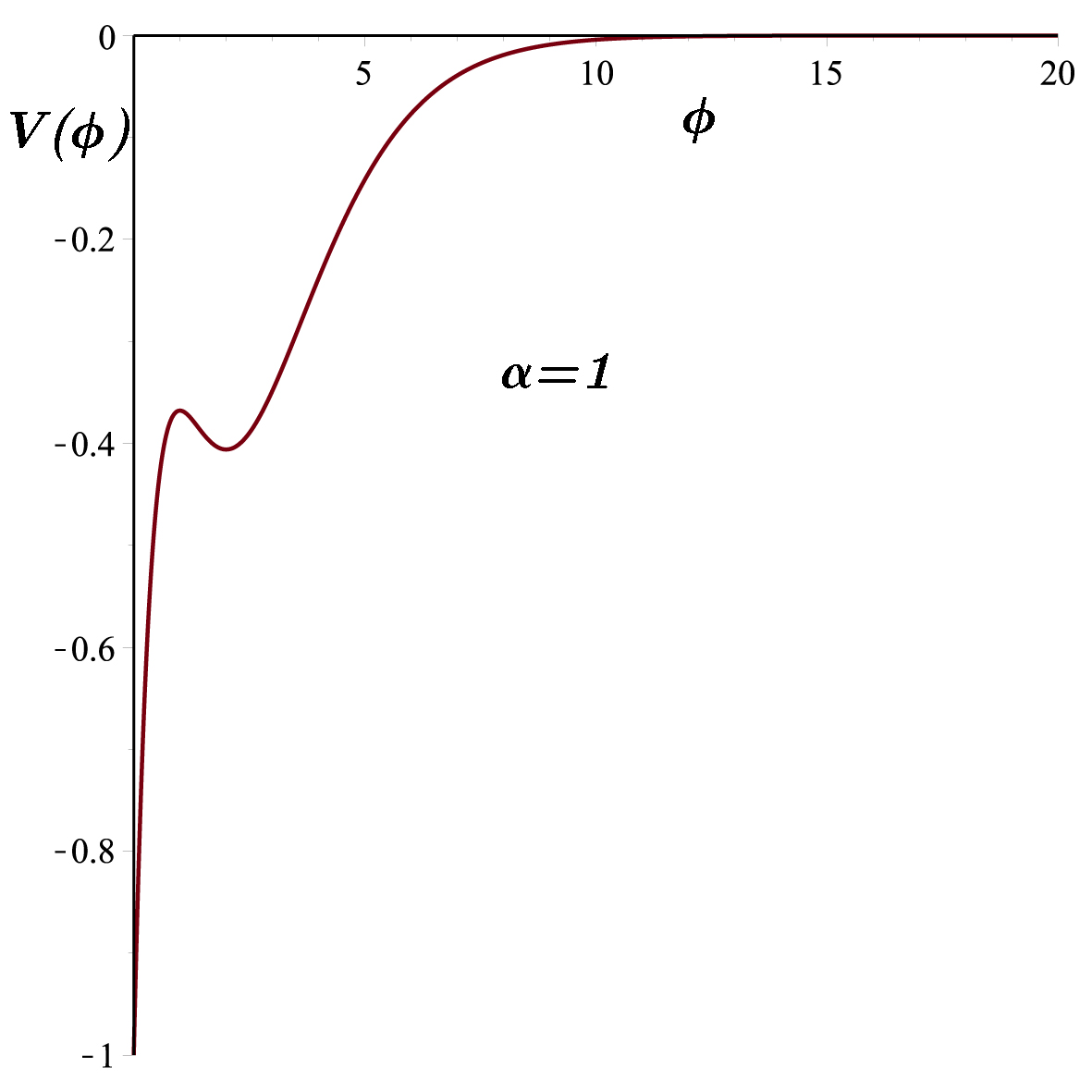
Figure 2: The self-coupling potential $V\left(\phi\right)$ versus $\phi$ for $M_{QL}=\frac{1}{12}$ and $\alpha=1.$ The minimum of the potential is the stability point of the scalar field (Eq. 27).

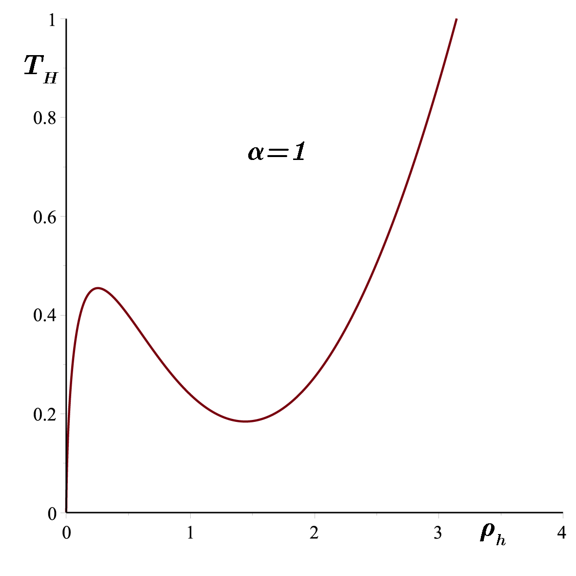
Figure 3: Hawking temperature $T_{H}$ versus the event horizon radius $\rho_{+}$ for $\alpha=1.$ The minimum of the Hawking temperature is observed (Eq. 47).

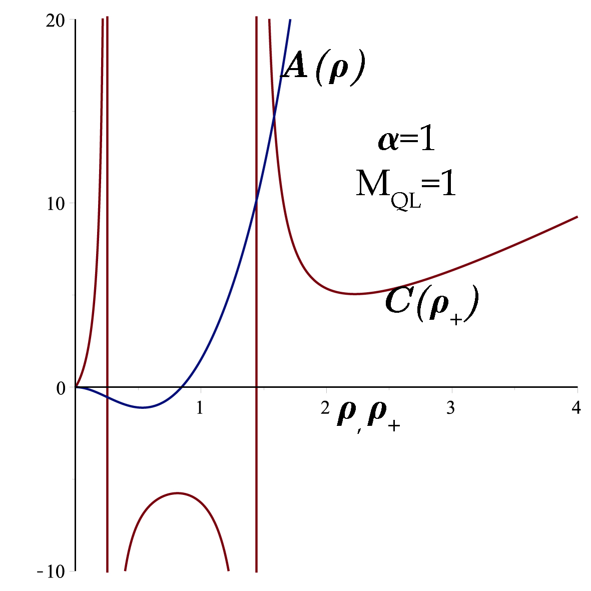
Figure 4: Specific heat $C$ versus the event horizon radius $\rho_{+}$ for $\alpha=1.$ Also the metric function $A\left(\rho\right)$ in terms of $\rho$ for $\alpha=1$ and $M_{QL}=1$ (Eqs. 43 and48).

III.1 Thermodynamics

The general solution found in the previous section is a two parameter solution which are $M_{QL}$ and $\alpha.$ The other integration constants are eliminated either by restriction or the fact that no new contribution they provide, see for instance $C_{1}$ and $C_{2}$ in (19). We should also admit that considering a relation between $H\left(r\right)$ and the scalar field in the form given in (18) imposes restriction to our general solution. As we stressed before, the solution may admit black hole with specific values for the free parameters $M_{QL}$ and $\alpha$. In such a case, let’s assume that the metric function $A\left(\rho\right)$ in (31) admits an event horizon located at $\rho=\rho_{+}.$ Using the standard definition of the Hawking temperature

$$T_{H}=\frac{1}{4\pi}\left.\sqrt{-g^{tt}g^{ij}g_{tt,i}g_{tt,j}}\right|_{\rho=\rho_{+}}$$ (38)

one finds

$$T_{H}=\frac{\left(\alpha^{2}+2\right)\rho_{+}^{\left(\frac{4}{\alpha^{2}}-2\right)}}{2\pi\alpha^{2}}\times\\ \left|\frac{\left(\alpha^{2}-2\right)^{2}\ln^{2}\rho_{+}+\alpha^{2}\left(\alpha^{2}-2\right)\ln\rho_{+}+\frac{\alpha^{4}}{2}}{\left(\alpha^{2}-2\right)^{3}}\right|.$$ (39)

Considering the entropy of the black hole at its horizon to be given by

$$S=\frac{A_{+}}{4}$$ (40)

with $A_{+}$ the surface area of the horizon, the specific heat

$$C=T_{H}\left(\frac{\partial S}{\partial T_{H}}\right)$$ (41)

yields

$$C=-\frac{\pi\alpha^{2}\rho_{+}}{2\left(\alpha^{2}-2\right)}\times\\ \frac{\left(\alpha^{2}-2\right)^{2}\ln^{2}\rho_{+}+\alpha^{2}\left(\alpha^{2}-2\right)\ln\rho_{+}+\frac{\alpha^{4}}{2}}{\left(\alpha^{2}-2\right)^{2}\ln^{2}\rho_{+}-\alpha^{2}\left(\alpha^{2}-2\right)\ln\rho_{+}-\frac{\alpha^{4}}{2}}.$$ (42)

We note that, thermodynamically the black hole is locally stable if $C$ is positive. Depending on the value of $\alpha$ and the radius of the horizon $\rho_{+},$ we may find stable $C>0$ or unstable $C<0$ black holes. This suggests that the value of $M_{QL}$ which contributes to the radius of the horizon, may be very crucial. In the case $\alpha=1$ in the following section we shall give an example.

III.2 Specific solution for $\alpha=1$

In this part we give the explicit solution for $\alpha=1.$ The metric function and the potential become

$$A\left(\rho\right)=-12M_{QL}\rho^{2}-9\rho\left(\ln^{2}\rho-2\ln\rho+\frac{3}{2}\right),$$ (43)

and

$$V\left(\phi\right)=-\left(1-\phi+\phi^{2}\right)e^{-\phi}$$ (44)

with

$$\phi=2\ln\rho.$$ (45)

Therefore the line element takes the form

$$ds^{2}=-A\left(\rho\right)dt^{2}+\frac{9\rho^{4}}{A(\rho)}d\rho^{2}+\rho^{2}d\theta^{2}.$$ (46)

The Hawking temperature is given by

$$T_{H}=\left|\frac{3\left(2\ln^{2}\rho_{+}-2\ln\rho_{+}+1\right)\rho_{+}}{4\pi}\right|,$$ (47)

and the specific heat reads

$$C=\frac{\pi\rho_{+}\left(\ln^{2}\rho_{+}-\ln\rho_{+}+\frac{1}{2}\right)}{2\left(\ln^{2}\rho_{+}+\ln\rho_{+}-\frac{1}{2}\right)}.$$ (48)

Fig. 1 is a plot of the metric function in terms of $\rho$ for $M_{QL}=\frac{1}{12},$ and $\alpha=1.$ For the same parameter values, in Fig. 2 we plot the potential $V$ in terms of $\phi$ which clearly shows a local minimum considered as the stability point of the field. In Fig. 3 we plot the Hawking temperature $T_{H}$ given by Eq. (47). In this figure we observe that a minimum temperature at certain horizon occurs. This horizon radius can be considered as the minimum energy state of the black hole which is more likely to admit a stable black hole. In Fig. 4, the specific heat $C$ and the metric function are displayed in terms of the event horizon $\rho_{+}$ and $\rho$ respectively for $\alpha=1.$ Let’s comment on this figure that as the horizon of this specific black hole is located in the region where the specific heat is negative, this black hole is not stable. The only parameter that can be changed to shift the horizon into the region with positive specific heat is the mass of the black hole i.e., $M_{QL}.$ Therefore increasing $M_{QL}$ causes the horizon to be larger and consequently one obtains a positive $C$ and a stable black hole.

III.3 A comparison with a singlet scalar field

For an analytical comparison between the doublet scalar field and the singlet scalar field one needs to consider in (1)

$$\mathcal{L}_{field}=-\frac{1}{2}\left(\nabla\phi\right)^{2}-V\left(\phi\right)$$ (49)

in which $\phi=\phi\left(r\right)$ is just a scalar field and $V\left(\phi\right)$ is given by (5). Having the line element (6), we find

$$\mathcal{L}_{field}=-\frac{A}{2}\phi^{\prime 2}-V\left(\phi\right)$$ (50)

and the scalar field equation is found to be

$$\phi^{\prime\prime}+\frac{\left(AH\right)^{\prime}}{AH}\phi^{\prime}-\frac{V^{\prime}\left(\phi\right)}{A}=0.$$ (51)

Einstein’s equations (9) with

$$T_{\mu}^{\nu}=\frac{1}{2}\left(\partial_{\mu}\phi\partial^{\nu}\phi-\frac{1}{2}\left(\nabla\phi\right)^{2}\delta_{\mu}^{\nu}\right)-\frac{1}{2}V\left(\phi\right)\delta_{\mu}^{\nu}$$ (52)

explicitly read

$$\frac{2H^{\prime\prime}A+A^{\prime}H^{\prime}}{H}+\frac{1}{2}A\phi^{\prime 2}+V=0,$$ (53)

$$\frac{A^{\prime}H^{\prime}}{H}-\frac{1}{2}A\phi^{\prime 2}+V=0$$ (54)

and

$$A^{\prime\prime}+\frac{1}{2}A\phi^{\prime 2}+V=0.$$ (55)

Combining the Einstein’s first two equations admits the same equation as (17) and the ansatz

$$H=e^{\mu\phi}$$ (56)

in which $\mu$ is a new constant parameter to be found, reveals a solution for $\phi$ given by

$$\phi\left(r\right)=\frac{2\mu}{2\mu^{2}+1}\ln r.$$ (57)

Having the first Einstein’s equation solved one finds $A\left(r\right)$ and making the other equations satisfied imposes $\xi_{1}=\xi_{2}=0$. Finally the closed form of the general solution to the field equations is given by

$$A\left(r\right)=C_{1}r^{\frac{4\mu^{2}}{2\mu^{2}+1}}+C_{2}r^{\frac{1}{2\mu^{2}+1}}$$ (58)

in which $C_{1}$ and $C_{2}$ are two integration constants. The final form of the potential, however, becomes

$$V=-\frac{2C_{1}\mu^{2}\left(4\mu^{2}-1\right)}{\left(2\mu^{2}+1\right)}e^{-\phi/\mu},$$ (59)

which indicates that $\mu=\frac{1}{\alpha}$ and $V_{0}=-\frac{2C_{1}\mu^{2}\left(4\mu^{2}-1\right)}{\left(2\mu^{2}+1\right)}$ when it is compared with (5). In terms of the parameters introduced in the potential function one may write the line element as

$$ds^{2}=-\left(\frac{V_{0}\left(2+\alpha^{2}\right)^{2}}{2\left(\alpha^{2}-4\right)}r^{\frac{4}{2+\alpha^{2}}}+C_{2}r^{\frac{\alpha^{2}}{2+\alpha^{2}}}\right)dt^{2}+\\ \frac{dr^{2}}{\frac{V_{0}\left(2+\alpha^{2}\right)^{2}}{2\left(\alpha^{2}-4\right)}r^{\frac{4}{2+\alpha^{2}}}+C_{2}r^{\frac{\alpha^{2}}{2+\alpha^{2}}}}+r^{\frac{4}{2+\alpha^{2}}}d\theta^{2}.$$ (60)

Let’s note that $\alpha=2$ must be excluded and the corresponding specific solution is given by

$$A\left(r\right)=r^{2/3}\left(C-3V_{0}\ln r\right)$$ (61)

with $H,$ $V$ and $\phi$ the same as the general $\alpha$ with $\alpha=2$ ($\mu=\frac{1}{2}$).

For the specific value of $\mu=\frac{1}{\sqrt{2}}$ ($\alpha=\sqrt{2}$) we find the line element to be

$$ds^{2}=-\left(C_{2}\sqrt{r}-4V_{0}r\right)dt^{2}+\frac{dr^{2}}{C_{2}\sqrt{r}-4V_{0}r}+rd\theta^{2}$$ (62)

which after the transformation $r=\rho^{2}$ becomes

$$ds^{2}=-\rho\left(C_{2}-4V_{0}\rho\right)dt^{2}+\frac{4\rho d\rho^{2}}{C_{2}-4V_{0}\rho}+\rho^{2}d\theta^{2}.$$ (63)

The scalar field and the potential read as

$$\phi=\sqrt{2}\ln\rho$$ (64)

and

$$V=\frac{V_{0}}{\rho^{2}}.$$ (65)

The solutions given by (56)-(59) represent three parameters solutions which are $\alpha,$ $C_{2}$ and $V_{0}.$ With proper choice of parameters the general solution (i.e., (58) or (61)) admits black hole solution. For instance, in the case $\alpha=\sqrt{2},$ if we assume that both $C_{2}$ and $V_{0}$ are negative the solution is a black hole with quasilocal mass given by the BY formalism (34) as

$$M_{QL}=\frac{\left|C_{2}\right|}{8}.$$ (66)

The differences between the singlet and doublet field equations as well as solutions are very clear. Finally let us add that by setting $C_{2}=0$ and $V_{0}=-1,$ the line element (63) becomes

$$ds^{2}=-\rho^{2}d\bar{t}^{2}+d\rho^{2}+\rho^{2}d\theta^{2}$$ (67)

where $\bar{t}=2t.$ This solution was found in 41 .

IV An extension to $3+1-$dimensions

In $3+1-$dimensions the action reads as

$$S=\int d^{4}x\sqrt{-g}\left(R+\mathcal{L}_{field}\right)$$ (68)

in which $\mathcal{L}_{field}$ is given by (2), however, the components of the triplet scalar potential as source are given by

$$\phi^{1} = \phi\left(r\right)\sin\theta\cos\varphi$$ (69)

$$\phi^{2} = \phi\left(r\right)\sin\theta\sin\varphi$$ (70)

$$\phi^{3} = \phi\left(r\right)\cos\theta$$ (71)

with its modulus given as in (4) with $a=1,2,3$. The self interacting potential is considered as $V\left(\phi\right)$ while the spherically symmetric line element is chosen to be

$$ds^{2}=-A\left(r\right)dt^{2}+\frac{1}{A(r)}dr^{2}+H\left(r\right)^{2}\left(d\theta^{2}+\sin^{2}\theta d\varphi^{2}\right).$$ (72)

Similar to the three dimensional case, the field equations are given by the variation of the action with respect to $\phi\left(r\right)$ which yields

$$\left(A\phi^{\prime}H^{2}\right)^{\prime}-2\phi=H^{2}V^{\prime}\left(\phi\right)$$ (73)

and with respect to the metric tensor which gives the Einstein’s equations with the energy-momentum tensor as in (10). These Einstein’s equations may be combined and in their simplest form they become

$$\left(A^{\prime}H^{2}\right)^{\prime}+H^{2}V=0,$$ (74)

$$4H^{\prime\prime}+H\phi^{\prime 2}=0,$$ (75)

$$A\left(H^{2}\right)^{\prime\prime}-H^{2}A^{\prime\prime}+\left(\phi^{2}-2\right)=0,$$ (76)

and

$$2\left(A^{\prime}HH^{\prime}+AH^{\prime 2}-1\right)-\left(\frac{AH^{2}\phi^{\prime 2}}{2}-\phi^{2}-H^{2}V\right)=0.$$ (77)

V Solution to the field equations in $3+1-$dimensions

One can check that the following set of functions for $\phi\left(r\right),$ $H\left(r\right),$ $A\left(r\right)$ and $V\left(\phi\right)$ satisfy all field equations,

$$\phi=\frac{2\alpha}{\alpha^{2}+1}\ln r,$$ (78)

$$H\left(r\right)=r^{\frac{\alpha^{2}}{\alpha^{2}+1}},$$ (79)

$$A\left(r\right)=-\frac{\Lambda}{3}r^{\frac{2\alpha^{2}}{1+\alpha^{2}}}-\frac{2M}{r^{\frac{\alpha^{2}-1}{\alpha^{2}+1}}}-\frac{2\alpha^{2}}{\left(\alpha^{4}-1\right)}r^{\frac{2}{\alpha^{2}+1}}\times\\ \left(\ln^{2}r-\frac{\alpha^{2}-3}{\alpha^{2}-1}\ln r-\frac{\alpha^{8}-3\alpha^{6}+4\alpha^{4}-7\alpha^{2}+1}{2\alpha^{2}\left(\alpha^{2}-1\right)^{2}}\right)$$ (80)

and

$$V\left(\phi\right)=\frac{2}{3}\frac{\alpha^{2}\left(3\alpha^{2}-1\right)\Lambda}{\left(\alpha^{2}+1\right)^{2}}e^{-\frac{\phi}{\alpha}}+\frac{2\left(2\alpha^{2}-1\right)}{\left(\alpha^{2}-1\right)^{3}}\times\\ \left(1+\frac{\alpha^{3}\left(\alpha^{2}-1\right)}{\left(2\alpha^{2}-1\right)}\phi+\frac{\left(\alpha^{2}-1\right)^{2}}{2\left(2\alpha^{2}-1\right)}\phi^{2}\right)e^{-\alpha\phi}.$$ (81)

Here, $\alpha$ is a free real parameter such that $\alpha\in\left[0,\infty\right)-\left\{1,\frac{1}{\sqrt{2}}\right\}$ while $M$ and $\Lambda$ are two integration constants corresponding to the mass of the black hole and the cosmological constant. Furthermore, in the limit $\alpha\rightarrow\infty$ one finds

$$\phi = 0,$$ (82)

$$H\left(r\right) = r,$$ (83)

$$A\left(r\right) = 1-\frac{\Lambda}{3}r^{2}-\frac{2M}{r}$$ (84)

and

$$V\left(\phi\right)=2\Lambda$$ (85)

which is the (anti) de-Sitter Schwarzschild black hole solution. Let’s add also that the limit $\alpha=0$ gives the Bertotti-Kasner spacetime 44 . Two particular cases corresponding to $\alpha=1$ and $\alpha=\frac{1}{\sqrt{2}}$ that were excluded above will be considered separately in the sequel. Before that we would like to look at the general solution more closely. First we apply the following transformation

$$r^{\frac{\alpha^{2}}{\alpha^{2}+1}}=x\text{ }$$ (86)

which yields

$$ds^{2}=-A\left(x\right)dt^{2}+\frac{\left(1+\frac{1}{\alpha^{2}}\right)^{2}x^{\frac{2}{\alpha^{2}}}dx^{2}}{A\left(x\right)}+x^{2}d\Omega^{2}$$ (87)

in which

$$A\left(x\right)=-\frac{\Lambda}{3}x^{2}-\frac{2M}{x^{1-\frac{1}{\alpha^{2}}}}-\frac{2\left(\alpha^{2}+1\right)^{2}x^{\frac{2}{\alpha^{2}}}}{\alpha^{2}\left(\alpha^{4}-1\right)}\times\\ \left(\ln^{2}x-\frac{\alpha^{2}\left(\alpha^{2}-3\right)\ln x}{\alpha^{4}-1}\right.\\ -\left.\frac{\left(\alpha^{8}-3\alpha^{6}+4\alpha^{4}-7\alpha^{2}+1\right)\alpha^{2}}{2\left(\alpha^{4}-1\right)^{2}}\right).$$ (88)

What we observe is that $\Lambda$ is still an effective cosmological constant and the spacetime admits black holes. Once more we apply the BY formalism to find the quasilocal mass of the possible central black hole. To do so we set $F\left(x_{B}\right)^{2}=A\left(x_{B}\right)$ and $G\left(x_{B}\right)^{2}=\frac{A\left(x_{B}\right)}{\left(1+\frac{1}{\alpha^{2}}\right)^{2}x_{B}^{\frac{2}{\alpha^{2}}}}$ in Eq. (34) which results in

$$M_{QL}=\frac{M}{\left(1+\frac{1}{\alpha^{2}}\right)}.$$ (89)

Clearly at the limit of $\alpha\rightarrow\infty$ the quasilocal mass reduces into ADM mass of the central Schwarzschild black hole. To complete our discussion on the solution given above, we add that the solution is singular only at the origin and it diverges as fast as $\frac{\ln^{3}x}{x^{4}}.$

V.1 Thermodynamics

Similar to the black hole solution in $2+1-$dimensions, here we determine some basic thermodynamic properties of the black hole solution given in (87) and (88). The Hawking temperature is found to be

$$T_{H}=\frac{x_{+}^{-\left(1+\frac{1}{\alpha^{2}}\right)}}{4\pi\alpha^{2}\left(1+\alpha^{2}\right)}\left|\alpha^{2}\Lambda\left(\alpha^{2}-\frac{1}{3}\right)x_{+}^{2}+\left(\alpha^{2}+1\right)^{2}x_{+}^{\frac{2}{\alpha^{2}}}\times\right.\\ \left.\frac{2\left(\alpha^{2}-1\right)^{2}\ln^{2}x_{+}+2\alpha^{2}\left(\alpha^{2}-1\right)\ln x_{+}-\alpha^{2}\left(\alpha^{4}-3\alpha^{2}+1\right)}{\left(\alpha^{2}-1\right)^{3}}\right|$$ (90)

in which $x_{+}$ is the radius of the event horizon. Having the entropy of the black hole to be

$$S=\pi x_{+}^{2}$$

and the definition of the specific heat (41), we determine

$$C=\frac{2\pi\alpha^{2}x_{+}^{2}}{\left(\alpha^{2}-1\right)}\times\\ \frac{\alpha^{2}\Lambda\left(\alpha^{2}-\frac{1}{3}\right)\left(\alpha^{2}-1\right)^{3}x_{+}^{2}-\Gamma_{1}\left(\alpha^{2}+1\right)^{2}x_{+}^{\frac{2}{\alpha^{2}}}}{\alpha^{2}\Lambda\left(\alpha^{2}-\frac{1}{3}\right)\left(\alpha^{2}-1\right)^{3}x_{+}^{2}+\Gamma_{2}\left(\alpha^{2}+1\right)^{2}x_{+}^{\frac{2}{\alpha^{2}}}},$$ (91)

where

$$\Gamma_{1}=-2\left(\alpha^{2}-1\right)^{2}\ln^{2}x_{+}-\\ 2\alpha^{2}\left(\alpha^{2}-1\right)\ln x_{+}+\alpha^{2}\left(\alpha^{4}-3\alpha^{2}+1\right)$$ (92)

and

$$\Gamma_{2}=-2\left(\alpha^{2}-1\right)^{2}\ln^{2}x_{+}+\\ 2\alpha^{2}\left(\alpha^{2}-1\right)\ln x_{+}+\alpha^{2}\left(\alpha^{4}-3\alpha^{2}+1\right).$$ (93)

We should add that, as of the $2+1-$dimensions, for a specific radius for the event horizon, depending on the sign of the heat capacity, the black hole, thermodynamically, is locally stable or unstable. In Fig. 5 we plot the specific heat $C\left(x_{+}\right)$ and the metric function $A\left(x\right)$ in terms of $x_{+}$ and $x$ respectively for $\alpha=2,$ $\Lambda=-4$ and $M_{QL}=1.$ Since $C$ is not a function of $M_{QL},$ changing the value of $M_{QL}$ does not alter $C$ however it changes the radius of the horizon. As in Fig. 5, for $M_{QL}=1$ the horizon located in the region where $C>0$ and as a result the black hole is stable. Decreasing $M_{QL}$ causes the horizon fall in the region where $C<0$ and the black hole is no longer stable.

In Fig. 6 we plot the Hawking temperature $T_{H}\left(x_{+}\right)$ and the metric function $A\left(x\right)$ in terms of $x_{+}$ and $x$ respectively for $\alpha=2,$ $\Lambda=-4$ and $M_{QL}=1.$ The Hawking temperature admits a zero and a local minimum.

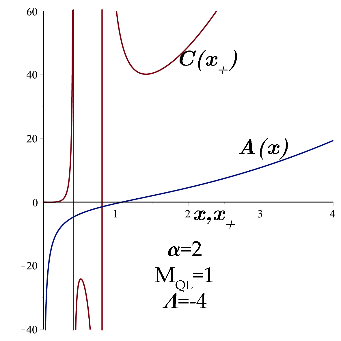
Figure 5: $C\left(x_{+}\right)$ and the metric function $A\left(x\right)$ in terms of $x_{+}$ and $x$ respectively for $\alpha=2,$ $\Lambda=-4$ and $M_{QL}=1$ (Eqs. 88 and 91).

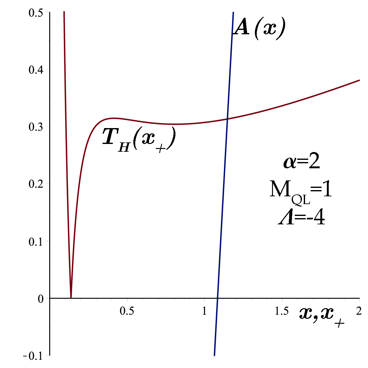
Figure 6: $T_{H}\left(x_{+}\right)$ and the metric function $A\left(x\right)$ in terms of $x_{+}$ and $x$ respectively for $\alpha=2,$ $\Lambda=-4$ and $M_{QL}=1$ (Eqs. 88 and 90).

V.2 $\alpha=1$

The solution for $\alpha=1$ which is obtained separately apart from the solution (78-81) becomes

$$\phi=\ln r,$$ (94)

$$H\left(r\right)=\sqrt{r},$$ (95)

$$A\left(r\right)=C_{2}+C_{1}r-r\ln^{2}r+\frac{r}{3}\ln^{3}r$$ (96)

and

$$V\left(\phi\right)=-\frac{1}{3}\left(3C_{1}-6-6\phi+3\phi^{2}+\phi^{3}\right)e^{-\phi}$$ (97)

in which $C_{1}$ and $C_{2}$ are two integration constants and the metric implies a non-asymptotically flat black hole solution. A coordinate transformation of the form $x=\sqrt{r}$ transforms the line element (69) into

$$ds^{2}=-A\left(x\right)dt^{2}+\frac{4x^{2}}{A\left(x\right)}dx^{2}+x^{2}d\Omega^{2}$$ (98)

with

$$A\left(x\right)=-4M_{QL}+C_{1}x^{2}-4x^{2}\ln^{2}x+\frac{8x^{2}}{3}\ln^{3}x.$$ (99)

Note that to find the quasilocal mass as $M_{QL}=\frac{-C_{2}}{4}$ we applied the BY formalism. Let’s add that the constant $C_{1}$ is an effective cosmological constant. In Fig. 7 we plot $V\left(\phi\right)$ versus $\phi$ for $C_{1}=0.$ In this figure we observe a kind of modified Mexican hat potential with the left minimum much deeper. In Fig. 8 we depict $A\left(x\right)$ versus $x$ for $C_{1}=0$ and $M_{QL}=1$ respectively.

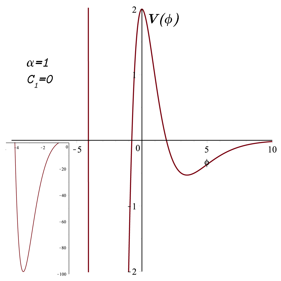
Figure 7: $V\left(\phi\right)$ versus $\phi$ for $C_{1}=0$ and $\alpha=1$ in $3+1$-dimensions i.e., Eq. (97).

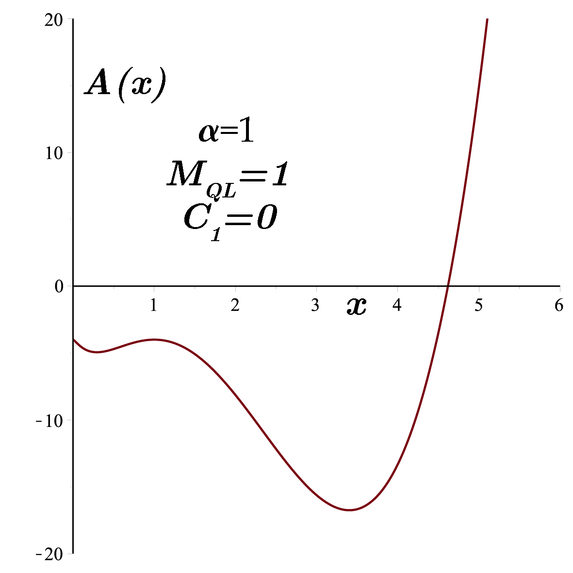
Figure 8: $A\left(x\right)$ versus $x$ for $C_{1}=0,$ $M_{QL}=1$ and $\alpha=1$ in $3+1$-dimensions i.e., Eq. (99).

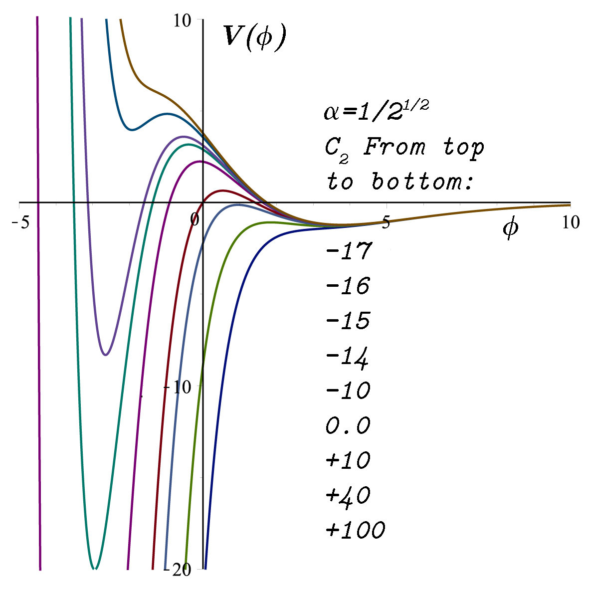
Figure 9: $V\left(\phi\right)$ versus $\phi$ for various values for $C_{2}$ and $\alpha=\frac{1}{\sqrt{2}}$ in $3+1$-dimensions i.e., Eq. (103).

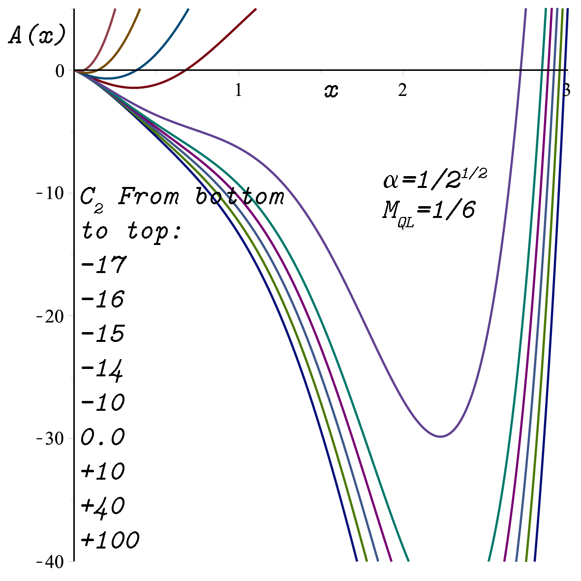
Figure 10: $A\left(x\right)$ versus $x$ for various values for $C_{2}$, $M_{QL}=\frac{1}{6}$ and $\alpha=\frac{1}{\sqrt{2}}$ in $3+1$-dimensions i.e., Eq. (106).

V.3 $\alpha=\frac{1}{\sqrt{2}}$

The solution for $\alpha=\frac{1}{\sqrt{2}}$ yields

$$\phi=\frac{2\sqrt{2}}{3}\ln r,$$ (100)

$$H\left(r\right)=\sqrt[3]{r},$$ (101)

$$A\left(r\right)=r^{\frac{2}{3}}C_{2}+C_{1}r^{\frac{1}{3}}+\frac{1}{3}r^{\frac{4}{3}}\left(29-20\ln r+4\ln^{2}r\right)$$ (102)

and

$$V\left(\phi\right)=-\frac{2}{9}C_{2}e^{-\sqrt{2}\phi}+2\phi\left(\sqrt{2}-\phi\right)e^{-\frac{\sqrt{2}}{2}\phi}$$ (103)

in which $C_{1}$ and $C_{2}$ are two integration constants. Once more we transform our solution by applying the following coordinate transformation

$$r=x^{3}$$ (104)

which modifies the line element into the form

$$ds^{2}=-A\left(x\right)dt^{2}+\frac{9x^{4}}{A\left(x\right)}dx^{2}+x^{2}d\Omega^{2}$$ (105)

where

$$A\left(x\right)=x^{2}C_{2}-6M_{QL}x+\frac{1}{3}x^{4}\left(29-60\ln x+36\ln^{2}x\right).$$ (106)

We add that from the BY formalism we found the quasilocal mass of the black hole solution as $M_{QL}=-\frac{C_{1}}{6}.$ In Fig. 9 we depicted $V\left(\phi\right)$ versus $\phi$ for various $C_{2}$ which is the effective cosmological constant. We observe that for a negative $C_{2}$ there is at most two local minima but for the positive values only one local minimum is found. In Fig. 10 we plot the corresponding metric function for $M_{QL}=\frac{1}{6}$.

VI Conclusion

By employing doublet and triplet of scalars with a self-interacting potential consisting only of their moduli we constructed classes of non-asymptotically flat black holes in $2+1-$ and $3+1-$ dimensions. The self-interacting potential consists of a polynomial term multiplied by a Liouville term. The latter factor is the potential which plays the role to dominate the asymptotic behaviors. Our model can be considered within the context of field theoretic black holes. Some thermodynamical properties including specific heat and quasilocal mass are given explicitly. The simplest member of our model is naturally the case of a constant potential term which corresponds to the cosmological constant. It is shown that the potential admits local minimum apt for the construction of suitable field theoretic black hole states. One distinguishing feature of our metric function obtained from scalar multiplets is that it is a polynomial of a mixture of radial function and its logarithms. It can be anticipated that given the proper self-interacting potential our model of multiplets can be extended to higher dimensions.  Unless this has been worked out explicitly, however, based only on $2+1$ / $3+1$ dimensions, it is hard to predict the higher dimensional behaviors and formulate a general no-go theorem in the presence of multiplet sources. In our restricted dimensions we obtained no asymptotically flat regular black hole solutions for $V\left(\phi\right)>0$, which is in conform with the no-go theorem introduced in 45 ; 46 .

References

• (1) M. Bañados, C. Teitelboim, J. Zanelli, Phys. Rev. Lett. 69, 1849 (1992).
• (2) M. Bañados, M. Henneaux, C. Teitelboim and J. Zanelli, Phys. Rev. D 48, 1506 (1993).
• (3) C. Martinez, C. Teitelboim and J. Zanelli, Phys. Rev. D 61, 104013 (2000).
• (4) S. Carlip, Quantum Gravity in 2 + 1-Dimensions, Cambridge University Press, 1998.
• (5) S. Carlip, Living Rev. Rel. 8, 1 (2005).
• (6) S. H. Mazharimousavi and M. Halilsoy, Phys. Rev. D 92, 024040 (2015).
• (7) S. H. Mazharimousavi and M. Halilsoy, Eur. Phys. J. C 75, 249 (2015).
• (8) A. L. Berkin and R. W. Hellings, Phys. Rev. D 49, 6442 (1994).
• (9) V. Vardanyan and L. Amendola, Phys. Rev. D 92, 024009 (2015).
• (10) M. Rainer and A. Zhuk, Phys. Rev. D 54, 6186 (1996).
• (11) D. I. Kaiser, Phys. Rev. D 81, 084044 (2010).
• (12) Y. Watanabe and J. White, Phys. Rev. D 92, 023504 (2015).
• (13) J. White, M. Minamitsuji and M. Sasaki, JCAP 07, 039 (2012).
• (14) K. Schutz, E. I. Sfakianakis and D. I. Kaiser, Phys. Rev. D 89, 064044 (2014).
• (15) D. H. Lyth and A. Riotto, Phys. Rep. 314, 1 (1999).
• (16) C. P. Burgess, Classical Quantum Gravity 24, S795 (2007).
• (17) L. McAllister and E. Silverstein, Gen. Relativ. Gravit. 40, 565 (2008).
• (18) D. Baumann and L. McAllister, Annu. Rev. Nucl. Part. Sci. 59, 67 (2009).
• (19) A. Mazumdar and J. Rocher, Phys. Rep. 497, 85 (2011).
• (20) M. Barriola and A. Vilenkin, Phys. Rev. Lett. 63, 341 (1989).
• (21) A. Vilenkin, Phys. Rep. 121, 263 (1985).
• (22) C. M. Chen, H. B. Cheng, X. Z. Li, X. H. Zhai, Class. Quantum Gravity 13, 701 (1996).
• (23) X. Z. Li, Commun. Theor. Phys. 28, 101 (1997).
• (24) D. Harari and C. Lousto, Phys. Rev. D 42, 2626 (1990).
• (25) O. Dando and R. Gregory, Class. Quantum Grav. 15, 985 (1998).
• (26) A. Banerjee, A. Beesham, S. Chatterjee and A. A. Sen, Class. Quantum Grav. 15, 645 (1998).
• (27) T. H. Lee and B. J. Lee, Phys. Rev. D 69, 127502 (2004).
• (28) R. M. Teixeira Filho and V. B. Bezerra, Phys. Rev. D 64, 067502 (2001).
• (29) T. Tamaki and K-ichi Maeda, Phys. Rev. D 60, 104049 (1999).
• (30) E. Hirschmann, Anzhong Wang, Y. Wu, Class. Quant. Grav. 21, 1791 (2004).
• (31) E. Ayón-Beato, A. Garcia, A. Macias, J. Perez-Sanchez, Phys. Lett. B 495, 164 (2000).
• (32) I. Z. Fisher, Z. Exp. Teor. Fiz. 18, 636 (1948).
• (33) T. Kodama, Phys. Rev. D 18, 3529 (1978).
• (34) T. Kodama, L. de Oliveira, F. Santos, Phys. Rev. D 19, 3576 (1979).
• (35) P. Baekler, E. Mielke, R. Hecht, F. Hehl, Nucl. Phys. B 288, 800 (1987).
• (36) K. Schmoltzi, T. Schücker, Phys. Lett. A 161, 212 (1991).
• (37) P. Jetzer, D. Scialom, Phys. Lett. A 169, 12 (1992).
• (38) T. Torii, K. Maeda, and M. Narita, Phys. Rev. D 64, 044007 (2001).
• (39) E. Winstanley, Found. Phys. 33, 111 (2003).
• (40) C. A. R. Herdeiro and E. Radu, Int. J. Mod. Phys. D 24, 1542014 (2015).
• (41) H.-J. Schmidt and D. Singleton, Phys. Lett. B 721, 294 (2013).
• (42) J. D. Brown and J. W. York, Phys. Rev. D 47, 1407 (1993).
• (43) J. D. Brown, J. Creighton and R. B. Mann, Phys. Rev. D 50, 6394 (1994).
• (44) W. Rindler, Phys. Lett. A, 245, 363 (1998).
• (45) K. A. Bronnikov and G.N. Shikin, Grav.Cosmol. 8, 107 (2002).
• (46) K. A. Bronnikov, S. B. Fadeev and A. V. Michtchenko, Gen. Rel. Grav. 35, 505 (2003).