Outflows and complex stellar kinematics in
SDSS star forming galaxies

We investigate the properties of star formation-driven outflows by using a large spectroscopic sample of $\sim$160,000 local “normal” star forming galaxies, drawn from the Sloan digital sky survey (SDSS), spanning a wide range of star formation rates (SFRs) and stellar masses (M_∗). The galaxy sample is divided into a fine grid of bins in the ${\rm M_{*}-SFR}$ parameter space, for each of which we produce a composite spectrum by stacking together the SDSS spectra of the galaxies contained in that bin. We exploit the high signal-to-noise of the stacked spectra to study the emergence of faint features of optical emission lines that may trace galactic outflows and would otherwise be too faint to detect in individual galaxy spectra. We adopt a novel approach that relies on the comparison between the line-of-sight velocity distribution (LoSVD) of the ionised gas (as traced by the [OIII]$\lambda$5007 and H$\alpha$+[NII]$\lambda\lambda$6548,6583 emission lines) and the LoSVD of the stars, which are used as a reference tracing virial motions. Significant deviations of the gas kinematics from the stellar kinematics in the high velocity tail of the LoSVDs are interpreted as a signature of outflows. Our results suggest that the incidence of ionised outflows increases with SFR and specific SFR. The outflow velocity ($v_{\rm out}$) is found to correlate tightly with the SFR for $\rm SFR>1\leavevmode\nobreak\ M_{\odot}\leavevmode\nobreak\ yr^{-1}$, whereas at lower SFRs the dependence of $v_{\rm out}$ on SFR is nearly flat. The outflow velocity, although with a much larger scatter, appears to increase also with the stellar velocity dispersion ($\sigma_{*}$), and we infer velocities as high as $v_{\rm out}\sim(6-8)\sigma_{*}$. Strikingly, we detect the signature of ionised outflows only in galaxies located above the main sequence (MS) of star forming galaxies in the M_∗–SFR diagram, and the incidence of such outflows increases sharply with the offset from the MS. This result suggests that star formation-driven outflows may be responsible for shaping the upper envelope of the MS by providing a self-regulating mechanism for star formation. Finally, our complementary analysis of the stellar kinematics reveals the presence of blue asymmetries of a few 10 km s^-1 in the stellar LoSVDs. The origin of such asymmetries is not clear, but a possibility is that these trace the presence, in local galaxies of a large number of high velocity runaway stars and hypervelocity stars in radial trajectories.

1 Introduction

Baryons in galaxies are engaged in a complex intertwining of mechanisms whose combined effects drive galaxy evolution. Key players of this game are gas, stars and active galactic nuclei (AGN). Gas is the primary ingredient of both star formation and black hole accretion, and its properties are therefore crucial for shaping galaxies. Star formation and AGN activity can in turn heavily influence the physical, chemical and kinematical conditions of gas within galaxies, thereby exerting a “feedback” on galaxy evolution. In a simplistic way, our current knowledge of the processes occurring in galaxies and involving gas and stars can be summarised as follows. The presence of gas within galaxies is a key prerequisite for star formation. In local galaxies, all known star formation takes place in dense molecular clouds, mostly in giant molecular clouds (GMCs, see review by Scoville 2013). The star formation process can be either smooth and quiescent, probably fostered by cosmological inflows of cold gas into galaxies (e.g. Dekel et al. 2009; Bouché et al. 2010), or bursty, triggered by dynamical processes such as galaxy interactions (Scoville, 2013). Recent studies suggested that the latter mode of star formation does not contribute significantly to the cosmic star formation rate (SFR) density, accounting for only 10% of it even at $z\sim 2$, i.e. the peak of the cosmic SFR density (Rodighiero et al., 2011). Although we still lack conclusive observational evidence for the presence of cold accretion flows feeding galaxy halos (but see promising observations by Cantalupo et al. 2014 and Hennawi et al. 2015 at $z\sim 2$), the hypothesis that the building up of baryonic mass is a secular process has been suggested by the observation of a tight correlation between stellar mass (${\rm M_{*}}$) and star formation rate in star forming galaxies (Bouché et al., 2010; Lilly et al., 2013), dubbed star formation “main sequence” (MS). The MS is a well-established property of the star forming galaxy population at $z\sim 0$ (Noeske et al., 2007; Peng et al., 2010) and is believed to persist at least up to $z\sim 4$ (Schreiber et al., 2015), with an intrinsic scatter of only $\sim 0.3$ dex.

Once star formation is activated, supernovae enrich the interstellar medium (ISM) with metals and, along with young and massive stars, inject energy and momentum into the ISM, thereby altering the physical conditions of the gas surrounding the sites of star formation and at the same time driving multi-phase galactic-scale outflows that propel part of the gas out of these regions, and in some cases can even expel it from the galaxy. The investigation of stellar feedback has triggered a wealth of both theoretical and observational works. For theoretical work we refer to the early review by Chevalier (1977) for energy-driven outflows, to Murray et al. (2005) for momentum-driven outflows, and to Hopkins et al. (2014) for cosmological zoom-in simulations exploring the combined effect of multiple stellar feedback mechanisms on galaxy evolution. For observational work we refer to the reviews by Veilleux et al. (2005) and Erb (2015), the latter one focussing on high redshift.

Gas heating and removal resulting from intense episodes of star formation is believed to play a key role in galaxy evolution. For example, stellar feedback may be the main responsible for: (i) the low efficiency of star formation observed in both low and high mass galaxies (Behroozi et al., 2010; Papastergis et al., 2012), although for more massive galaxies an additional feedback from AGNs is often invoked (e.g. reviews by Cattaneo et al. 2009 and Kormendy & Ho 2013); (ii) the lower gas-phase metal content of low-mass galaxies with respect to more massive galaxies (Davé et al., 2011a), and (iii) the consequent enrichment of the circumgalactic medium (CGM) with metals (Mac Low & Ferrara, 1999). Moreover, it has been suggested that galactic outflows driven by star formation may have aided the reionization of the early Universe, by creating gas-free paths around young star clusters thus facilitating the leakage of ionising photons from the first galaxies (Heckman et al., 2011; Erb, 2015).

Although blueshifted absorption lines at optical and UV wavelengths are probably the most direct and accessible tool to identify outflows of ionised (and atomic) gas, especially in distant galaxies, nebular emission lines such as [OIII]$\lambda$5007, H$\alpha$ and [NII]$\lambda\lambda$6548,6584 are also widely employed to study galactic outflows, both in local star forming galaxies (e.g. Heckman et al. 1990; Veilleux et al. 1995; Lehnert & Heckman 1996; Soto et al. 2012; Westmoquette et al. 2012; Rupke & Veilleux 2013; Rodríguez Zaurín et al. 2013; Bellocchi et al. 2013; Cazzoli et al. 2014; Arribas et al. 2014) and at higher redshifts (e.g. Shapiro et al. 2009; Newman et al. 2012; Harrison et al. 2012; Cano-Diaz et al. 2012; Genzel et al. 2014; Förster Schreiber et al. 2014; Carniani et al. 2015). However, despite the increasing number of observational studies targeting galactic outflows and the remarkable advances in the field, a systematic and unbiased investigation of star formation-driven outflows in a large sample of galaxies is still missing. Indeed, since the outflow signature can be very faint and difficult to detect in individual normal galaxies, previous studies focused on rather small samples, mostly characterised by “extreme” properties (e.g. powerful and massive starbursts, ultra-luminous infrared galaxies (ULIRGs)), hence not representative of the general galaxy population, although significant improvement has been recently made in this regard (e.g. Chen et al. 2010; Martin et al. 2012; Rubin et al. 2014; Chisholm et al. 2014).

In this paper we study star formation-driven outflows of ionised gas as traced by faint broad wings of optical emission lines ([OIII]$\lambda$5007, H$\alpha$ and [NII]$\lambda\lambda$6548,6584) by using the largest and most unbiased spectroscopic sample of local galaxies currently available, the Sloan digital sky survey (SDSS). The SDSS, in conjunction with the catalogues provided by the MPA-JHU analysis, constitutes a huge database, whose noteworthy potential in terms of studying the general properties of galaxies can be further exploited by stacking multiple spectra together to obtain very high signal-to-noise composite spectra (e.g. Chen et al. 2010; Andrews & Martini 2013). The stacking technique has numerous advantages, and it is particularly useful when searching for faint spectral features, such as those impressed by galactic outflows, which can be missed in the noise of single galaxy spectra.

We divide the ${\rm M_{*}-SFR}$ parameter space into a fine grid of bins, each of which includes from several tens to thousands of sources. The spectra within each bin are then stacked together to produce a single, very high signal-to-noise composite spectrum that is representative of the spectrum of a “typical” galaxy in that bin, in which we can study the emergence of faint broad wings of optical emission lines that may trace ionised outflows. Moreover, since stellar mass and star formation rate are intrinsically correlated in most star-forming galaxies (because most of them follow the MS), by stacking galaxies in bins of SFR and M_∗ we can investigate the trends between the outflow properties and these two parameters independently, thus breaking their degeneracy resulting from the MS. The SDSS database and the use of the stacking technique allow us to explore the incidence and properties of ionised outflows over a wide dynamical range of galaxy properties, i.e. ${\rm M_{*}\in[2\times 10^{7},6\times 10^{11}]\leavevmode\nobreak\ M_{\odot}}$ and ${\rm SFR\in[2\times 10^{-3},2\times 10^{2}]\leavevmode\nobreak\ M_{\odot}\leavevmode\nobreak\ yr^{-1}}$, which is unprecedented in outflow studies.

A rather controversial issue in studies of galactic outflows through emission line profiles is the definition of “broad component”, which is supposed to trace gas in outflow, and of “narrow component”, which instead traces virial motions in the galaxy. Such an issue has not been addressed in a systematic way by previous studies: most of them just rely on the $\chi^{2}$ improvement to establish the necessity of a broad component to fit the emission line profile (e.g. Harrison et al. 2012; Westmoquette et al. 2012; Bellocchi et al. 2013; Arribas et al. 2014). Moreover, even if a broad component is present, its association with galactic flows is not straightforward: a broad component in emission may trace the high velocity tail of virialised motions within the galaxy, or galaxy interactions. In this study we attempt to overcome this problem by adopting a novel strategy, consisting in directly comparing the line-of-sight velocity distribution (hereafter, LoSVD) of the ionised gas with the LoSVD of the stars, which is taken as a reference tracing virial motions. Accordingly, gaseous outflows are identified by deviations of the gas kinematics from the stellar kinematics, and in particular by the presence of an excess of gas velocity with respect to the stars in the high velocity tail of the LoSVD.

Summarising, the main goal of this work is to investigate the incidence and properties of galactic outflows of ionised gas as a function of a wide range of galaxy properties, breaking the degeneracy between SFR and ${\rm M_{*}}$. Moreover, for the first time, we push outflow studies to stellar masses and SFRs as low as ${\rm 2\times 10^{7}\leavevmode\nobreak\ M_{\odot}}$ and ${\rm 2\times 10^{-3}M_{\odot}\leavevmode\nobreak\ yr^{-1}}$, respectively, a regime that has not been probed before in this field.

A ${\rm H_{0}}$ = 70 km s^-1 Mpc^-1, ${\rm\Omega_{M}}$=0.27, ${\rm\Omega_{\Lambda}}$=0.73 cosmology is adopted throughout this paper.

Figure 1: The SDSS sample of star-forming, non active galaxies selected for this study, plotted in the M_∗-SFR parameter space. The grid of 50 bins used for the stacking is shown, with the bins colour-coded according to the number of spectra enclosed. The exact number of sources within each bin is indicated by the yellow text. The white dashed and dotted lines represent the MS relation of local star-forming galaxies with its $\pm 1\sigma$ scatter ($=0.3$ dex). The MS relation has been taken from Peng et al. (2010) and adapted to this dataset as explained in $\S$ 2.2.

2 Methods

In this section we present the SDSS sample of star forming, non active galaxies selected for this study ($\S$ 2.1). We also describe in detail the stacking procedure ($\S$ 2.2) and the fitting techniques applied to the stellar continuum and to the [OIII]$\lambda$5007 and H$\alpha$+[NII]$\lambda\lambda$6548,6583 nebular lines to obtain the line-of-sight velocity distributions of stars and ionised gas from the galaxy composite spectra ($\S$ 2.3- 2.6).

2.1 Sample selection

Our galaxy sample is entirely drawn from the spectroscopic sample of the Sloan digital sky survey, data release 7 (SDSS DR7, Abazajian et al. 2009). We operate a first selection by including only those galaxies enclosed in the MPA-JHU catalogue , which provides intrinsic and derived spectral parameters for each source, such as redshift, emission line fluxes, stellar mass, and star formation rate (Tremonti et al., 2004; Kauffmann et al., 2003; Brinchmann et al., 2004; Salim et al., 2007). The MPA-JHU analysis encompasses only SDSS DR7 sources at $z<0.7$.

Among the MPA-JHU galaxies, we selected only sources classified as “star-forming” (or “HII”) according to their location on the log([OIII]/H$\beta$) vs log([NII]/H$\alpha$) diagram (i.e. the “BPT” diagram, Baldwin et al. 1981), by adopting the same division criteria as Kauffmann et al. (2003). Such selection is needed in order to avoid contamination from AGNs, which is of primary importance to constrain the star formation-driven feedback mechanisms in action in normal local galaxies.

We note that the BPT selection may introduce a potential bias in our sample of star forming galaxies. This is due to the fact that purely star forming galaxies may still exhibit extended areas where the optical line ratios are typical of low-ionisation emission line regions (LINERs). As a consequence, an “HII” galaxy may be erroneously classified as “Composite” or “LINER” when its optical emission is averaged over a large aperture (such as the SDSS spectroscopic fibre). Extended LINER-like gas excitation in purely star forming galaxies can have different origins. In the vast majority of local isolated (inactive) galaxies, the most plausible source of extended LINER-type excitation are evolved (post-AGB) stars (Cid Fernandes et al., 2011; Yan & Blanton, 2012; Singh et al., 2013; Belfiore et al., 2015). This is in general not the case for strongly star forming galaxies such as (U)LIRGs, where there is evidence for extended LINER excitation associated with widespread shocks. Indeed, both theoretical models (Allen et al., 2008) and spatially resolved integral field spectroscopy (IFS) observations (Monreal-Ibero et al., 2006, 2010; Soto & Martin, 2012; Rich et al., 2014, 2015) have shown that galaxy regions dominated by shock excitation exhibit optical line ratios typical of LINERs.

Since extended shocks can be associated with strong outflows produced by vigorous star formation (e.g. Sharp & Bland-Hawthorn 2010), our sample selection, by leaving out LINERs and Composite galaxies, may be biased against (U)LIRGs experiencing strong feedback from star formation. Although this is certainly a caveat to keep in mind, the nature of the widespread shocks that may dominate the ionised gas excitation over extended regions in (U)LIRGs is most likely linked to the merger process. This argument is based on the lack of observational evidence for shock-like excitation significantly affecting the optical line fluxes in isolated (U)LIRGs (Monreal-Ibero et al., 2010; Rich et al., 2015). Indeed, the point made by resolved IFS studies (Soto & Martin, 2012; Rich et al., 2014, 2015) about a possible misclassification of star forming galaxies hosting widespread shocks, when aperture-integrated spectra are used, concerns only (U)LIRGs in a merger stage. In contrast, for isolated (U)LIRGs, the contribution from shocks to extended optical line emission is negligible (Monreal-Ibero et al., 2010; Rich et al., 2015). Therefore, the types of shocks that can affect integrated optical line fluxes to the point that an “HII” galaxy is classified as “Composite” or “LINER” are galaxy-wide shocks produced by a complex interplay of merger-driven processes, and not just by star-formation-driven outflows. For their sample of local ULIRGs, Monreal-Ibero et al. (2006) explicitly concluded that the LINER-type optical line ratios observed in the extranuclear regions, several kiloparsecs away from the circumnuclear starburst, are due to shocks associated with tidally-induced large-scale flows produced during the merger and not to star formation-driven “superwinds” (which instead tend to dominate the gas kinematics in the inner regions of these ULIRGs that are characterised mostly by HII-type excitation). A similar conclusion was reached by Monreal-Ibero et al. (2010) who investigated the excitation source of ionised gas in a sample of 32 local LIRGs using IFS data, and found that the presence and relevance of shock-type excitation is more strongly correlated with the interaction class of the system than with the star formation activity (with isolated galaxies being largely dominated by HII-type excitation).

In summary, based on the observational evidence available from IFS studies, our BPT sample selection could lead to two possible biases: (i) a bias against ageing isolated galaxies dominated by old stellar populations and/or (ii) a bias against merger-driven shocks. The first bias would affect massive “retired” galaxies with stellar populations older than 1 Gyr and little ongoing star formation (e.g. Cid Fernandes et al. 2011; Singh et al. 2013), hence with very little or no star formation feedback at work. The second bias would affect mergers, which are only a minor fraction of the local galaxy population (Patton & Atfield, 2008) and so unimportant in our sample. Moreover, even if hypothesising that our analysis under-represents merging (U)LIRGs experiencing strong feedback, our conclusions (e.g. $\S$ 4.2) would not be affected but would actually be even strengthened: in this case we would be under-representing galaxies with high SFRs/sSFRs (i.e. galaxies above the Main Sequence in the M_∗-SFR diagram, e.g. Combes et al. 2013; Kilerci Eser et al. 2014) with strong outflows, hence our investigation and the relevant results could be regarded as conservative.

In addition to the BPT selection of “HII” galaxies, we require a signal-to-noise greater than five in all four emission lines used in the BPT diagram (i.e. [OIII], H$\beta$, [NII], H$\alpha$). As a consequence, the most passive galaxies, which do not show prominent nebular lines, are under-represented in our sample. We note that, by imposing a threshold SNR on the [OIII] and [NII] line fluxes, we may introduce a bias with metallicity. However, since local galaxies define a tight surface in the $\rm M_{*}-\mathcal{Z}-SFR$ plane (i.e. the “fundamental metallicity relation”, e.g. Mannucci et al. 2010; Lara-López et al. 2010), we do not expect galaxies within a given bin in the $\rm M_{*}-SFR$ parameter space to show significant variations in metallicity. Therefore, the main effect of imposing SNR constraints on the [OIII] and [NII] emission lines is that our sample selection does not allow us to populate certain regions of the $\rm M_{*}-SFR$ parameter space, but we are not introducing differential biases within the galaxy bins that are included in our sample.

A general caveat for this study is that at the median redshift of our sample, $z_{\rm med}$ = 0.073, the 3 arcsec-diameter of the SDSS spectroscopic fibre samples only the galaxy emission within $r\lesssim 2.1$ kpc. Moreover, the spectroscopic fibre samples a wide range of different projected sizes within our galaxy sample. Aperture effects are an obvious limitation of our study that will need to be taken into account in future works and that can be tackled properly only by using spatially-resolved observations. In order to be able to study outflows in “normal” galaxies (i.e. in galaxies that are neither extreme starbursts nor AGN hosts) we need to wait for the completion of ongoing large IFS surveys such as the CALIFA, SAMI and MaNGA surveys, although these will still have a statistics that is orders of magnitudes smaller than that provided by the SDSS. Another potential source of bias is given by galaxy inclination, which can have an important effect on the detectability of outflows (e.g. Chen et al. 2010). However, in terms of outflow properties, we expect the stacking of thousands of spectra to average out the effects of inclination, and so we do not expect our results to be greatly affected.

Our final selection consists of 157,639 galaxy spectra, whose distribution in the ${\rm M_{*}-SFR}$ diagram is shown in Fig. 1. The stellar mass of each galaxy was derived from a fit to the observed spectral energy distribution (SED), obtained with SDSS broad-band photometry (Brinchmann et al., 2004; Salim et al., 2007), which therefore takes into account the total emission from the galaxy. The SFR estimate is instead based on the H$\alpha$ intrinsic luminosity following the procedure described by Brinchmann et al. (2004), without applying any aperture correction to the SDSS fibre-limited spectrum: the SFRs employed in this work are therefore the “fibre SFRs” provided in the MPA-JHU catalogue. Such choice is justified by the fact that, in this study, we infer the properties of the gaseous and stellar kinematics by using exclusively the information provided by the fibre-limited SDSS spectroscopy, hence we do not have information on the gas (and so on possible outflows) on scales larger than those sampled by the fibre. Therefore, we believe that, given the obvious limitations of SDSS spectroscopy (which can be overcome only with IFS studies), it is more sensible to look for possible correlations between the properties of ionised outflows (on the scales sampled by the SDSS fibre) and the fibre SFRs, rather than the aperture-corrected SFRs. For the stellar mass instead we have chosen to use the “total” M_∗ because galactic outflows are expected to feel the effect of the entire galaxy gravitational potential well, which is linked to the total stellar mass.

2.2 Stacking procedure

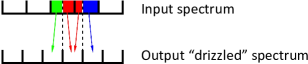
Figure 2: Sketch of the “Drizzle” method applied to the SDSS spectra.

The ${\rm M_{*}-SFR}$ parameter space sampled by our SDSS galaxy selection is divided into a fine grid of 50 bins, as shown in Fig. 1, and the spectra within each bin are stacked together to obtain very high signal-to-noise composite spectra. Each bin is required to include a minimum of 50 sources, but most bins contain over 100 galaxies, and the central ones up to $\sim 20,000$. Throughout this paper, we will code each stack by its average log(SFR) and log(M_∗) (ID=log(SFR)_log(M_∗)).

We also show in Fig. 1 the position of the main sequence of local star-forming galaxies and its $\pm 0.3$ dex scatter (Salim et al., 2007; Peng et al., 2010). Since we use fibre-limited SFRs, the reference MS for this study differs slightly from the MS relationship derived by Peng et al. (2010), who instead used aperture-corrected SFRs. The main effect of using SFRs that are not corrected for the SDSS aperture is a downward shift of the MS relation by $\rm\Delta log(SFR)=-0.4$ dex. This shift was estimated by selecting, in our sample, galaxies with $0.02<z<0.085$ (to match the redshift range of Peng et al. 2010) and $\rm 9.0<log(M_{*}[M_{\odot}])<11.0$ (i.e. the stellar mass range where the mean relationship between log(SFR) and log(M_∗) is linear) and by fitting the mean trend between log(SFR) and log(M_∗) with a linear relationship, whose slope was constrained to be the same as Peng et al. (2010). However, we stress that the aim of this work is not to provide a “general” fit to the local MS relation of star-forming galaxies, and that the MS relationship shown in Fig. 1 should only be used as a reference for this galaxy sample. We refer to the works by Peng et al. (2010); Schreiber et al. (2015) and Gavazzi et al. (2015) for more detailed discussion about the MS of star forming galaxies.

Prior to stacking, the galaxy spectra in each bin are de-reddened and normalised to their extinction-corrected H$\beta$ line flux, which is related to the star formation rate in the galaxy. The reddening $E(B-V)$ is estimated from the observed H$\alpha$-to-H$\beta$ flux ratio, by using the Galactic extinction curve as described in Cardelli et al. (1989) and by assuming $R_{V}=A_{V}/E(B-V)=3.1$. The spectra are then shifted to the rest-frame by using the redshifts provided by the Princeton-1D spectroscopic pipeline and contextually re-binned by using a technique based on “Drizzle”, the method for linear reconstruction of under-sampled images (Fruchter & Hook, 2002). The drizzling consists in mapping the original redshifted SDSS spectrum into a rest-frame pixel grid (the output spectrum) by taking into account their different pixel sizes and relative shift, as sketched in Fig. 2. In practice, the flux contained in the input pixel is averaged into the output pixel with a weight that is proportional to the area of overlap between the two pixels. The resulting spectra have a wavelength separation of 0.8 Å pixel^-1, i.e. slightly finer than the original SDSS spectra. The rest-frame galaxy spectra in each bin are finally averaged together to produce a single composite spectrum (the final stack), which is then normalised to its mean.

2.3 Stellar subtraction

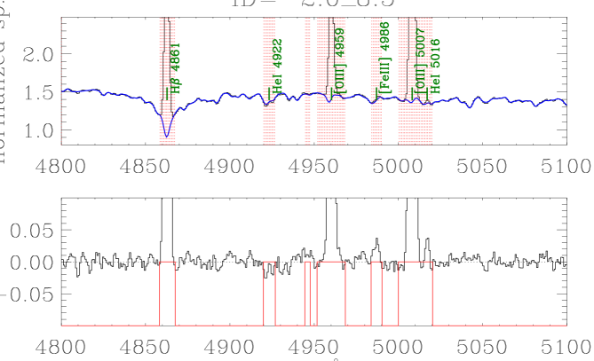
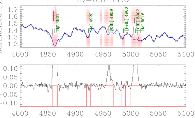
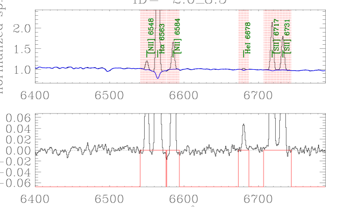
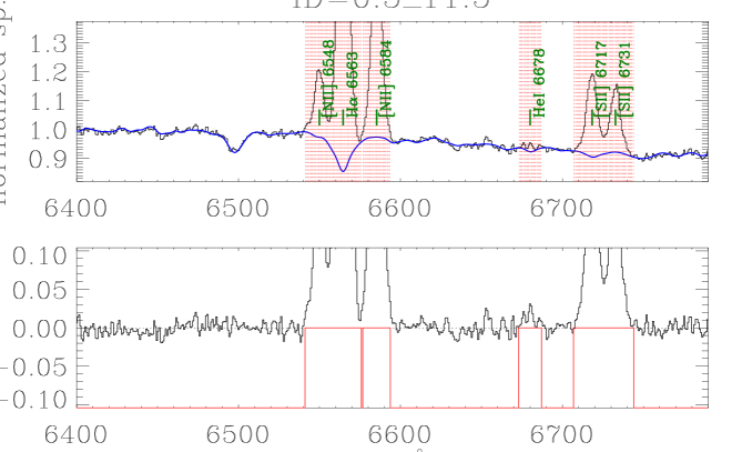
Figure 3: Stellar continuum fit and subtraction over two wavelength ranges including the [OIII]$\lambda 5007$ emission line (top panels) and the H$\alpha$+[NII] emission lines (bottom panels), performed for two galaxy stacks: ID=-2.0_8.5 (left) and ID=0.5_11.5 (right). In each plot, the upper panel shows the stacked spectrum (black) and the best fit to the stellar continuum (blue), while the lower panel shows the residual spectrum. The red shaded regions mark the spectral windows containing nebular features and therefore masked from the stellar continuum fit.

The subtraction of the stellar continuum emission from the stacked spectra is of crucial importance for this study, which is aimed at detecting faint wings of nebular emission lines. For the purpose of stellar subtraction, we select as stellar templates a large set of synthetic spectra of single stellar populations (SSPs) computed with the PÉGASE-HR v3.0 code (Le Borgne et al., 2004), with both low metallicities ($\mathcal{Z}=0.004$) and solar metallicities ($\mathcal{Z}=0.02$). The PÉGASE-HR spectral templates cover the wavelength range $\lambda\in[4000,6800]$ Å, with a spectral resolving power of $R=10,000$ at $\lambda=5500$ Å, and are computed for a wide range of ages (from 10 Myr to 2 Gyr), by assuming a Salpeter initial mass function (IMF, Salpeter 1955).

We fit the PÉGASE-HR templates to the nebular line-free regions of the composite galaxy spectra by using the IDL implementation of the penalised pixel-fitting (pPXF) method developed by Cappellari & Emsellem (2004). The stellar continuum fitting and subtraction is performed in two wavelength ranges, i.e. $\lambda\in[4800,5100]$ Å and $\lambda\in[6200,6790]$ Å, selected to include the [OIII]$\lambda$5007 and the H$\alpha$ +[NII]$\lambda\lambda$6548,6583 nebular emission lines, which are the targets of this study. The nebular emission lines and ISM absorption features are masked from the stellar fit to prevent it from being affected by non-stellar features. When the fit is provided with a large enough number of stellar features in the non-masked portion of the spectrum (which is always true in the spectral region we are interested in), this procedure can accurately determine the stellar contamination under the masked nebular lines. Figure 3 shows the stellar continuum fit and subtraction performed for two different stacks. We note that the pPXF procedure, together with the high resolution PÉGASE-HR templates, produces an excellent fit to the stellar continuum underlying the nebular features in the galaxy stacks.

2.4 SDSS spectral instrumental profile

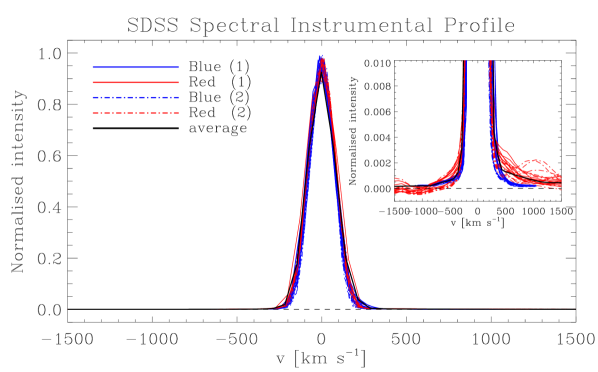
Figure 4: Instrumental profile of the SDSS spectrographs, estimated from bright, non-blended emission lines in the arc lamp images, selected within the wavelength range of interest for this study (i.e. HgI $\lambda$5460.753 Å for the blue cameras and NeI $\lambda$6598.953 Å for the red cameras). For each camera (blue/red) of the two spectrographs (1/2), we overplotted ten representative profiles from as many different frames (corresponding to different plates) obtained by averaging the arc lamp spectra over all 320 fibres. The black solid line corresponds to the mean profile. The inset highlights the presence of low-level instrumental wings (corresponding to $\lesssim 3/1000$ of the peak), which are more prominent for the red cameras.

Our investigation of the kinematics of the ionised gas in local star forming galaxies, as traced by the [OIII]$\lambda$5007 and H$\alpha$+[NII]$\lambda\lambda$6548,6583 nebular emission lines, is aimed at finding broad wings of the LoSVD of the ionised gas that may be signature of outflows. This is done by comparing, in each galaxy stack, the LoSVD of the gas with the LoSVD of the stars. As it will be explained in $\S$ 2.5, the LoSVD of the stars is derived by fitting the stellar continuum around $\lambda=5500$ Å, i.e. in a spectral region where the stellar fit produces the best results thanks to the large number of stellar absorption lines and the scarcity of nebular (ISM) features. However, in order to extract the real kinematics of stars and gas from the observed line profiles (either from the nebular emission lines, in the case of the gas, or from the stellar features seen in absorption, in the case of the stars), the LoSVDs of gas and stars must be deconvolved from the instrumental spectral profile. Therefore, it is of primary importance for our study to determine the instrumental profile of the SDSS spectrographs.

The presence of scattered light in the spectrometer may affect the spectral instrumental profile, resulting in extended wings. For the purpose of our investigation, we use the arc lamp calibration spectra to retrieve and analyse the spectral instrumental profile of the original SDSS spectrographs (adopted for SDSS-II). The average SDSS instrumental profile profile, shown in Fig. 4, is impressively clean from wings down to $\lesssim 3/1000$ of the peak, where some low-level instrumental wings start to appear. This effect is however negligible for our study, since it clearly cannot account for the much stronger broad (and asymmetric) line wings that we detect in our galaxy stacks, as it will be shown in $\S$ 3.

Smee et al. (2013) analyse, in their Figure 35, the spectral resolving power ($R(\lambda)=\lambda/(2.35*\sigma_{\lambda})$) of the original SDSS spectrographs as a function of wavelength. The resolving power of SDSS is quite difficult to constrain between $\lambda=5000$ Å and $\lambda=6000$ Å, because in this spectral region $R$ does not depend monotonically on wavelength, due to the transition from the blue to the red camera of the spectrographs (and some overlap between the two). In this study we adopt $R=1850$ (corresponding to ${\rm\sigma_{v}=69\leavevmode\nobreak\ km\leavevmode\nobreak\ s^{-1}}$), which is the average spectral resolving power inferred from the arc lamp images (Figure 4) and is on the lower side of (but still well within) the nominal range quoted in the literature for the SDSS spectrographs (i.e. $R\in[1800,2000]$).

2.5 The LoSVD of the stars

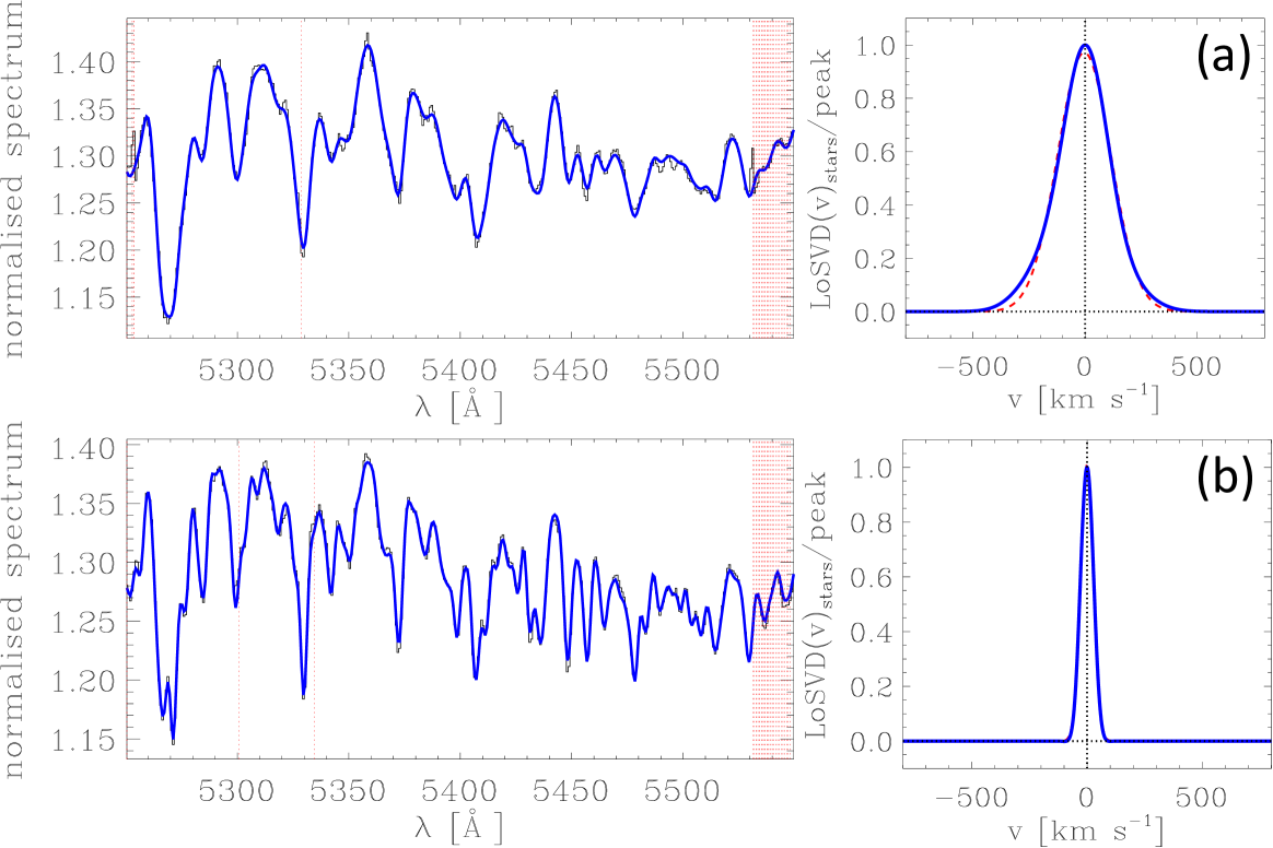
Figure 5: Stellar continuum fit over the range ${\rm\lambda\in[5250,5550]\leavevmode\nobreak\ \AA{}}$ (left) and resulting stellar LoSVD (right) derived for two galaxy stacks, i.e. $\rm ID=-0.5\_11.0$ (panel a) and $\rm ID=-1.5\_9.5$ (panel b). In the left panels, the stacked spectrum is plotted in black, and the best fit to the stellar continuum is in blue. The red dashed regions mark the spectral windows masked from the stellar continuum fit because of the presence of nebular features. In the right panels, the red dashed line indicates the LoSVD profile obtained by using, in the pPXF procedure, a simple Gaussian function to model the stellar features, while the blue solid line shows the stellar LoSVD profile obtained by allowing the use of Hermite polynomials to account for possible asymmetries of the stellar absorption features (Cappellari & Emsellem, 2004). The stellar LoSVD obtained for the stack $\rm ID=-0.5\_11.0$ shows a clear blue asymmetry. The fit is excellent (${\chi_{\rm red}^{2}}$ = 0.8) for both stacks.

The pPXF method developed by Cappellari & Emsellem (2004) allows us not only to accurately fit the stellar continuum and subtract it from the stacked spectra of galaxies, but also to extract the stellar kinematics. The pPXF procedure adopts a Gauss-Hermite parametrisation for the stellar line-of-sight velocity distributions, which accounts for possible asymmetries in the stellar absorption line profiles.

To infer the stellar LoSVDs, we first convolve the stellar templates (i.e. the PÉGASE-HR synthetic spectra) with the SDSS instrumental spectral profile obtained in $\S$ 2.4. When performing the stellar continuum fit by using these stellar templates (i.e. the ones convolved with the instrumental profile), the pPXF procedure yields the “real” stellar LoSVD, i.e. the stellar LoSVD deconvolved from the instrumental profile. As already mentioned in $\S$ 2.4, in order to extract the stellar kinematics, it is preferable to perform the continuum fitting around $\lambda\sim 5500$ Å, because this spectral region is abundant in stellar absorption features and relatively free of nebular emission lines. For this reason, to infer the stellar LoSVDs, we fit the stellar continuum in wavelength ranges selected between $\lambda=5100$ Å and $\lambda=5850$ Å or between $\lambda=6050$ Å and $\lambda=6250$ Å. The range $\lambda\in[5850,6050]$ Å is avoided because of the presence of the NaID $\lambda\lambda$5890,5896 Å resonance absorption doublet, which is contaminated by the galaxy ISM.

An example of continuum fitting aimed at extracting the stellar kinematics is reported in Fig. 5 for two different galaxy stacks, i.e. $\rm ID=-0.5\_11.0$ and $\rm ID=-1.5\_9.5$. We note that the $\rm ID=-0.5\_11.0$ stack shows a significant asymmetry in its stellar LoSVD. The presence of asymmetries in the stellar LoSVDs has been evidenced also in other stacks and will be discussed in $\S$ 3.3.

2.6 The LoSVD of the ionised gas

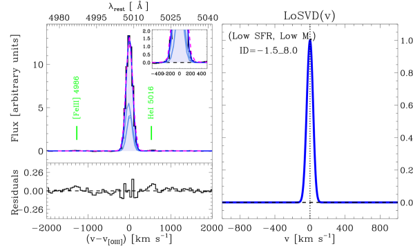
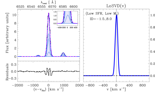
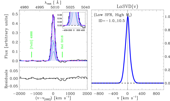
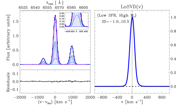
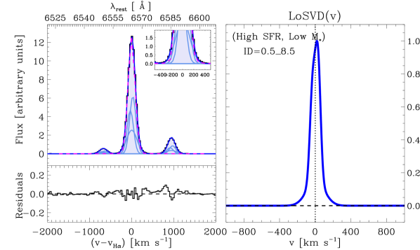
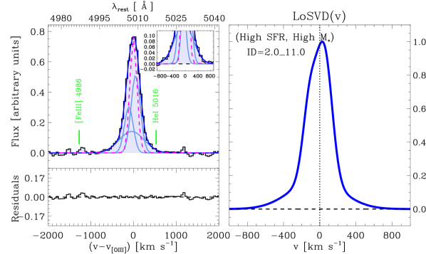
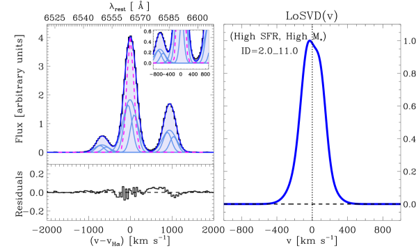
Figure 6: Examples of spectral fits to the [OIII]$\lambda$5007 (left column) and H$\alpha$+[NII] (right column) emission line profiles for four representative galaxy bins with different SFR and M_∗. From top to bottom: ID=-1.5 8.0 (low SFR and low M_∗), ID=-1.0 10.5 (low SFR and high M_∗), ID=0.5 8.5 (high SFR and low M_∗), and ID=2.0 11.0 (high SFR and high M_∗). In each plot, the left panel shows the fit to the data (solid curves, the total fit is in blue, the multiple Gaussian components in a lighter shade of blue). For comparison, we have overplotted to the data the average SDSS instrumental resolution profile (magenta dashed curve, from Fig. 4). In the right panel of each plot we show the final LoSVD of the ionised gas resulting from the fit, hence deconvolved from the SDSS instrumental profile (details in $\S$ 2.6).

Figure 7: Same as Fig. 6 but for a typical bin on the MS, with intermediate SFR and M_∗ (ID=0.0 10.5).

To infer the LoSVD of the ionised gas we fit, for each stack, the [OIII]$\lambda$5007, H$\alpha$ and [NII]$\lambda\lambda$6548,6583 emission lines with a function that results from the convolution of the SDSS instrumental profile, $\mathcal{R}(v)$, with another function $\mathcal{L}(v)$, which by definition corresponds to the “real” LoSVD of ionised gas. To account for potential broad wings of the LoSVD, possibly tracing outflows of ionised gas, $\mathcal{L}(v)$ is parametrised by the sum of three Gaussians, $l_{k}(v)$ ($k=$1,2,3), each centred at a velocity $v_{0,k}$, with area $a_{k}$ and standard deviation $\sigma_{k}$, i.e.

$$\mathcal{L}(v)=\sum_{k=1}^{3}l_{k}(v)=\sum_{k=1}^{3}a_{k}\,n_{k}\,e^{-(v-v_{0,k})^{2}/2\sigma_{k}^{2}},$$ (1)

where $n_{k}=1/\sqrt{2\pi\sigma_{k}^{2}}$ is the normalisation factor. Therefore, the “observed” LoSVD, $F(v)$, resulting from the convolution of the “real” LoSVD ($\mathcal{L}(v)$) and the SDSS spectral resolution profile ($\mathcal{R}(v)$), is given by:

$${F(v)=\mathcal{L}(v)\ast\mathcal{R}(v)=\sum_{k=1}^{3}l_{k}(v)\ast\mathcal{R}(v)=\sum_{k=1}^{3}f_{k}(v)},$$ (2)

where we have used the distributive property of the convolution (indicated by the symbol $\ast$) and we have defined $f_{k}(v)\equiv l_{k}(v)\ast\mathcal{R}(v)$. As a result, since both $l_{k}(v)$ and $\mathcal{R}(v)$ are Gaussians, $f_{k}(v)$ has the form:

$$f_{k}(v)=a_{k}\,N_{k}\,e^{-(v-v_{0,k})^{2}/2(\sigma_{k}^{2}+\sigma_{R}^{2})},$$ (3)

with ${N_{k}}=1/\sqrt{2\pi(\sigma_{k}^{2}+\sigma_{R}^{2})}$.

An emission line centred at a velocity ${v_{i}}$, corresponding to a central wavelength $\lambda_{i}$, will be fitted with a final function of the form:

$${\mathcal{F}_{i}(\lambda)=F(v)\ast[\varphi_{i}\leavevmode\nobreak\ \delta(v-v_{i})]=F(v)\ast\Biggl{[}\varphi_{i}\leavevmode\nobreak\ \delta\Bigl{(}c\frac{\lambda-\lambda_{i}}{\lambda_{i}}\Bigr{)}\Biggl{]}},$$ (4)

that is, the observed LoSVD, $F(v)$, convolved with a Dirac delta function centred at the vacuum wavelength of the line ${\lambda_{i}}$ and whose integral ${\varphi_{i}}$ is proportional to the line flux. Following Eq. 4, the final function ${\mathcal{F}_{[OIII]}(\lambda)}$ that we employ to fit the [OIII]$\lambda$5007 emission line profile in the composite spectra is:

$${\mathcal{F}_{[OIII]}(\lambda)}=\\ {\varphi_{[OIII]}\sum_{k=1}^{3}a_{k}N_{k}\,e^{-\bigl{[}\frac{c(\lambda-\lambda_{[OIII]})}{\lambda_{[OIII]}}-v_{0,k}\bigr{]}^{2}\bigl{/}2\bigl{(}\sigma_{k}^{2}+\sigma_{R}^{2}\bigr{)}}}.$$ (5)

Similarly, we fit the H$\alpha$+[NII] emission lines with a function of the form:

$${\mathcal{F}_{tot}(\lambda)=\mathcal{F}_{H\alpha}(\lambda)+\mathcal{F}_{[NII]6548}(\lambda)+\mathcal{F}_{[NII]6583}(\lambda)}=\\ {\varphi_{H\alpha}\sum_{k=1}^{3}a_{k}N_{k}\,e^{-\bigl{[}\frac{c(\lambda-\lambda_{H\alpha})}{\lambda_{H\alpha}}-v_{0,k}\bigr{]}^{2}\bigl{/}2\bigl{(}\sigma_{k}^{2}+\sigma_{R}^{2}\bigr{)}}}+\\ {\varphi_{[NII]}\sum_{k=1}^{3}a_{k}N_{k}\,e^{-\bigl{[}\frac{c(\lambda-\lambda_{H\alpha})}{\lambda_{H\alpha}}-\frac{c(\lambda_{[NII]}-\lambda_{H\alpha})}{\lambda_{H\alpha}}-v_{0,k}\bigr{]}^{2}\bigl{/}2\bigl{(}\sigma_{k}^{2}+\sigma_{R}^{2}\bigr{)}}}+\\ {3\varphi_{[NII]}\sum_{k=1}^{3}a_{k}N_{k}\,e^{-\bigl{[}\frac{c(\lambda-\lambda_{H\alpha})}{\lambda_{H\alpha}}-\frac{c(\varrho\lambda_{[NII]}-\lambda_{H\alpha})}{\lambda_{H\alpha}}-v_{0,k}\bigr{]}^{2}\bigl{/}2\bigl{(}\sigma_{k}^{2}+\sigma_{R}^{2}\bigr{)}}}.$$

In this equation, [NII] indicates the bluest line of the [NII] doublet, i.e. the [NII]$\lambda$6548 line, and $\varrho$ denotes the theoretical ratio between the rest-frame vacuum wavelengths of the [NII]$\lambda$6548 and [NII]$\lambda$6583 lines as reported in the NIST database.

The kinematics (velocity and widths) of all components fitting the H$\alpha$+[NII] complex is set to be equal for the three transitions. Such a constrained approach is necessary to separate the partially blended H$\alpha$ and [NII] emission lines and it improves the quality and reliability of the fit, as pointed out by Westmoquette et al. (2012). Moreover this method is justified by the fact that in star forming galaxies and in absence of strong shocks, the H$\alpha$ and [NII] emission lines arise from adjacent regions.

The fit, whose input parameters are only the instrumental resolution (${\sigma_{R}}$) and the (vacuum) central wavelengths of the different transitions (${\lambda_{i}}$), provides us with the relative line fluxes ${\varphi_{i}}$ and with other nine parameters, i.e. $v_{0,k}$, $\sigma_{k}$ and $a_{k}$ (with the index ${k=1,2,3}$ denoting the three Gaussian components used to model the observed LoSVD) from which, using Eq. 1, we retrieve ${\mathcal{L}(v)}$, i.e. the real LoSVD of the ionised gas. Figures 6 and 7 show example fits to the [OIII]$\lambda$5007 and H$\alpha$+[NII] emission lines as well as the resulting LoSVDs, for five representative galaxy stacks, having different SFR and M_∗ properties (in particular, low and high SFR, low and high M_∗, and intermediate SFR and M_∗). In Figs. 6 and 7 we also show for comparison, over-plotted to the observed spectral emission line profiles, the average SDSS instrumental profile (from Fig. 4), to show that the broad asymmetric wings we detected in a few of the stacks (e.g. ID=2.0 11.0) are not instrumental.

3 Results

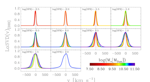
Figure 8: Line-of-sight velocity distribution of the ionised gas as traced by the [OIII]$\lambda$5007 emission line. In each panel we have over-plotted the LoSVDs of galaxy bins identified by the same (average) SFR and by different (average) stellar masses, colour-coded by their M_∗.

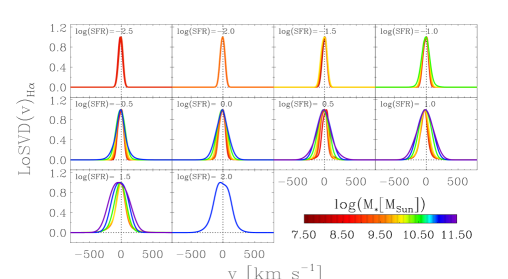
Figure 9: Line-of-sight velocity distribution of the ionised gas as traced by the H$\alpha$+[NII] emission lines. In each panel we have over-plotted the LoSVDs of galaxy bins identified by the same (average) SFR and by different (average) stellar masses, colour-coded by their M_∗.

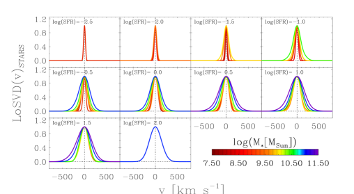
Figure 10: Line-of-sight velocity distribution of the stars. In each panel we have over-plotted the LoSVDs of galaxy bins identified by the same (average) SFR and by different (average) stellar masses, colour-coded by their M_∗.

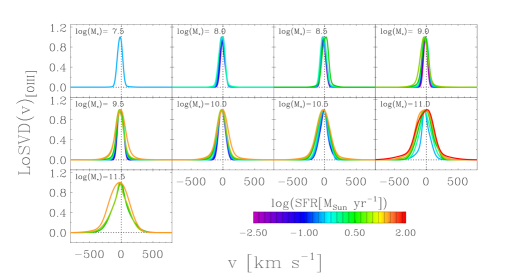
Figure 11: Line-of-sight velocity distribution of the ionised gas as traced by the [OIII]$\lambda$5007 emission line. In each panel we have over-plotted the LoSVDs of galaxy bins identified by the same (average) M_∗ and by different (average) SFRs, colour-coded by their SFR.

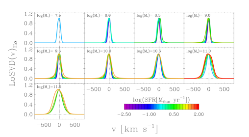
Figure 12: Line-of-sight velocity distribution of the ionised gas as traced by the H$\alpha$+[NII] emission lines. In each panel we have over-plotted the LoSVDs of galaxy bins identified by the same (average) M_∗ and by different (average) SFRs, colour-coded by their SFR.

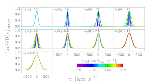
Figure 13: Line-of-sight velocity distribution of the stars. In each panel we have over-plotted the LoSVDs of galaxy bins identified by the same (average) M_∗ and by different (average) SFRs, colour-coded by their SFR.

In this section we present the results of our analysis of the dynamical properties of ionised gas and stars based on stacked SDSS spectra of local star-forming galaxies, aimed at identifying the presence of galactic outflows. Throughout the remainder of the paper and in the figures, for the sake of simplicity, we will replace “[OIII]$\lambda$5007” and “H$\alpha$+[NII]$\lambda\lambda$6548,6583” with “[OIII]” and “H$\alpha$”, respectively. The reader should however keep in mind that “H$\alpha$” actually refers to the H$\alpha$ and [NII] line complex as a whole, since the LoSVDs were derived by fitting the H$\alpha$ and [NII] lines simultaneously, as explained in $\S$ 2.6. The adopted strategy is briefly summarised in $\S$ 3.1. In $\S$ 3.2 we analyse the general properties of the LoSVDs of gas and stars; in $\S$ 3.3 we study the presence of asymmetric wings in the LoSVD profiles and finally in $\S$ 3.4 we discuss the outflow properties.

3.1 The novelty of our approach

Before presenting our results, we first shortly summarise what is new in our approach to the study of galactic outflows, by emphasizing the advantages and strengths of this method. For the first time, we study galactic outflows by directly comparing the LoSVD of the ionised gas (as traced by the [OIII], H$\alpha$ and [NII] nebular emission lines) with the LoSVD of the stars. This has never been attempted before, primarily because previous studies could not reach the signal-to-noise needed to extract the stellar LoSVDs from the data, and (if any) they just relied on the comparison between the velocity dispersion of gas and stars.

Furthermore, this technique holds the potential of detecting the signature of outflows in sources spanning a wide dynamic range of physical parameters as shown in Fig. 1, and in particular in faint, low mass (i.e. ${\rm M_{*}}$ as low as ${\rm\sim 2\times 10^{7}\leavevmode\nobreak\ M_{\odot}}$) and moderately star-forming (i.e. SFR as low as ${\rm\sim 2\times 10^{-3}\leavevmode\nobreak\ M_{\odot}\leavevmode\nobreak\ yr^{-1}}$) galaxies. The main limitations when probing outflows in galaxies having such low stellar masses and low star formation rates with SDSS spectroscopy are both the low signal-to-noise and low spectral resolution of the associated spectra. In this study, however, we overcome both these limitations. Firstly, we use the stacking technique to significantly improve the signal-to-noise in the spectra ($\S$ 2.2). Secondly, we minimise problems associated with the limited spectral resolution by deconvolving the “real” line-of-sight velocity distribution of gas and stars from the instrumental spectral profile in the observed resolution-limited composite spectra (as described in $\S$ 2.4-$\S$ 2.6). This is made possible thanks to the high signal-to-noise of the stacked spectra, especially for those galaxy bins in which the observed line profiles are narrow (i.e. line widths are close to the instrumental resolution). In particular, since, in emission lines, outflows are traced by a broad component superimposed on a narrow component, our deconvolution technique in principle allows us to detect such a broad component, provided it is broad enough, even if the bulk of the (narrow) emission line is not resolved.

3.2 Properties of the kinematics of gas and stars

LoSVD profiles

In the following we analyse variations in the LoSVD profiles of (ionised) gas and stars as a function of stellar mass and star formation rate. We stress that, since the galaxy spectra have been stacked in bins of ${\rm M_{*}}$ and SFR, the trends with ${\rm M_{*}}$ and SFR can be investigated independently, thus breaking the degeneracy between SFR and M_∗ that holds for star forming galaxies on the MS. For each stack, we adopt the velocity corresponding to the peak of the stellar LoSVD as a reference zero velocity for the LoSVD of both the stars and the gas.

Figures 8, 9 and 10 show the variations of the LoSVD profiles of gas and stars as a function of ${\rm M_{*}}$ at a fixed SFR. The most obvious trend that emerges from these figures is the increasing width of the LoSVDs of both gas and stars with stellar mass at a given SFR. This is simply a consequence of the fact that, to first order, the velocity dispersion of both gas and stars primarily traces virial motions that are related to the dynamical mass of the galaxy. The dynamical mass of a galaxy is, to first order, proportional to its stellar mass, although also gas and dust contribute to it. Therefore, broader LoSVDs are expected at higher stellar masses, simply because higher stellar masses are generally associated with higher dynamical masses. A comparison between Fig. 8 and 9 shows that the [OIII] and the H$\alpha$ LoSVD profiles are overall consistent.

The stellar LoSVDs in Fig. 10 show some interesting properties: they are overall quite broad, and have wings that extend up to several hundreds of km s^-1 in velocity, similar to the ionised gas traced by [OIII] and H$\alpha$, in particular for bins with ${\rm-0.5\leq log(SFR[M_{\odot}\leavevmode\nobreak\ yr^{-1}])\leq 1.5}$. This is in part a consequence of the velocity tail of the stellar distribution, but additional effects may be present, and these will be discussed in detail later in this section.

Figures 11, 12 and 13 are complementary to Figs. 8, 9 and 10: they show the trends of LoSVD profiles of gas and stars as a function of SFR for fixed M_∗. We first focus on Figs. 11 and 12: at a given stellar mass, the LoSVDs of [OIII]- and H$\alpha$-emitting gas broaden at higher SFRs. Such broadening is particularly evident for the “wings” of the line-of-sight velocity distributions, especially at stellar masses between ${\rm 9.0\leq log(M_{*}[M_{\odot}])\leq 11.0}$ for the [OIII] LoSVDs, and between ${\rm 9.0\leq log(M_{*}[M_{\odot}])\leq 10.0}$ for the H$\alpha$ LoSVDs. As we will discuss later in this section, the overall broadening of the LoSVDs of ionised gas observed with increasing SFR at fixed M_∗ could trace various stellar feedback-related phenomena, such as turbulence in the disk gas and outflows.

A dependency of the width of the LoSVD on the SFR is also seen in the stars (Figure 13), although in a smaller measure and especially at lower stellar masses (i.e. ${\rm log(M_{*}[M_{\odot}])\leq 10.5}$) than, for example, in the [OIII] LoSVDs (Figure 11). In the case of the stars, the LoSVD broadening with SFR (for constant ${\rm M_{*}}$) may be associated with an increase of the total dynamical mass of the systems. In particular, the increase in width of the stellar LoSVDs is possibly tracing an increase of the total gas content in galaxies with higher SFRs, which is in turn a consequence of the Schmidt–Kennicutt relation between SFR and total gas mass surface density (Schmidt, 1959; Kennicutt, 1998). However, this trend might be affected by a potential observational bias: the average projected size of galaxies decreases for higher SFRs (higher SFRs correspond, on average, to more distant sources because of selection effects), and this may have an effect on the stellar velocity dispersion measured within the SDSS fibre.

The line-of-sight velocity distributions of [OIII] and H$\alpha$ (Figures 8, 9, 11, and 12) exhibit asymmetries between the blue and the red side of the profiles. By eye inspection, such asymmetries appear to depend on the SFR, but a more quantitative analysis will be presented in $\S$ 3.3. We note that, quite surprisingly, also the stellar LoSVDs in Fig. 10 and 13 appear, although to a smaller extent, asymmetrical; such an effect can be best appreciated in bins with ${\rm log(SFR\leavevmode\nobreak\ [M_{\odot}yr^{-1}])=0.5}$ and ${\rm log(SFR\leavevmode\nobreak\ [M_{\odot}yr^{-1}])=1.5}$ (Figure 10). Asymmetries of the LoSVDs of gas and stars will be investigated in $\S$ 3.3.

LoSVD parameters: $\sigma$ and percentile velocities

The next step is to extrapolate physically meaningful quantities from the LoSVDs of stars and gas, and investigate the relationships with galaxy properties. Errors on the LoSVD parameters are obtained using the bootstrap technique (Efron, 1979). The bootstrap method consists in randomly resampling (with replacements) our galaxy stacks, by generating, for each bin, resampled stacks with sample size (here indicated with $S$) equal to the original stack. More specifically, for each bin in the $\rm M_{*}-SFR$ parameter space (Figure 1), we produce $N\gg 1$ resampled stacks, each of which is obtained by randomly selecting $S$ galaxy spectra from the original sample of $S$ spectra included in that bin and by co-adding them to produce a new “resampled” stack. The difference from the original stack is that, in the resampled stacks, the $S$ spectra to be co-added together are extracted randomly from the parent sample of $S$ galaxy spectra by allowing repetitions, hence the spectrum of a given galaxy can be selected either once, or more than once, or never. After producing $N$ resampled stacks for each bin, we perform for each of them the stellar continuum subtraction and the [OIII] and H$\alpha$+[NII] line fitting, exactly in the same way as for the original stacks (see $\S$ 2.3, $\S$ 2.5 and $\S$ 2.6), in order to retrieve the LoSVDs of stars and gas. Therefore, the bootstrap provides, for each bin and for a given LoSVD parameter of interest ($p_{i}$), a distribution of $N$ values. The variance of this distribution of $N$ parameters (following on from the variance of the galaxy samples) is used to estimate the error on the measure of $p_{i}$. The choice of the number $N$ of resampled stacks for each bin is a compromise between statistics and computational effort. We set $N=10$ for the most crowded bins, i.e. those including $S\geq 10,000$ galaxy spectra, $N=50$ for bins with $5,000\leq S<10,000$, and $N=100$ for the remaining ones, i.e. those with less than 5,000 objects.

The simplest parameter to study is the line-of-sight velocity dispersion ($\sigma$), given by:

$$\sigma=\biggl{(}\int(v-v_{c})^{2}\mathcal{L}(v)dv\biggr{)}^{1/2},$$ (6)

where the line-of-sight velocity distribution described by ${\mathcal{L}(v)}$ is normalised such as ${\int\mathcal{L}(v)dv=1}$, and $v_{c}$ is the centroid of the distribution, i.e. ${v_{c}=\int v\leavevmode\nobreak\ \mathcal{L}(v)\textit{d}v}$. The relationships between $\sigma$ (of both the ionised gas, as traced by [OIII] and H$\alpha$ and the stars), and galaxy properties such as SFR, M_∗ and sSFR (sSFR = SFR/${\rm M_{*}}$, i.e. star formation rate per stellar mass unit) are shown in Fig. 14.

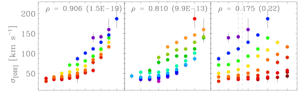
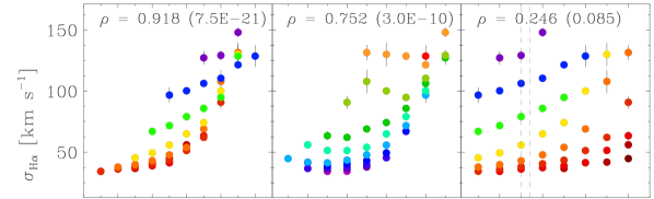
Figure 14: Line-of-sight velocity dispersion of the ionised gas as traced by the [OIII] (top panel) and H$\alpha$ (middle panel) emission lines, and of the stars (bottom panel). The errors were obtained by applying the bootstrap method, as explained in the text. The grey dashed lines in the third column mark the sSFR range corresponding to the MS of local star-forming galaxies between ${\rm 9.0\leq log(M_{*}[M_{\odot}])\leq 11.0}$. The Spearman rank correlation coefficient ($0<\rho<1$, higher values of $\rho$ indicate stronger correlation) is reported in each plot, along with the corresponding two-sided p-value as given in parenthesis (if the p-value is $\leq\alpha$, where $\alpha=0.05$ is the level of significance, the observed correlation is statistically significant).

For each plot in Fig. 14, we calculated the non-parametric Spearman rank correlation parameter ($\rho\in(0,1)$) to test the hypothesis of correlation between the line-of-sight velocity dispersion of gas and stars and the galaxy properties (SFR, M_∗, sSFR). In our case, non-parametric tests such as the Spearman rank test are more appropriate than the standard Pearson correlation coefficient ($r$), since we are dealing with binned data and the relationship between $\sigma$ and galaxy properties (if any) could be non-linear. A high value of $\rho$ (e.g., $\rho\gtrsim 0.5$) combined with a low p-value ($\leq\alpha$, where $\alpha$ is the level of significance, which we set $\alpha=0.05$) indicates the presence of a statistically significant correlation. In the calculation of the p-value, we allow for both positive and negative correlations (“two-sided”). The results of the Spearman rank test are reported in Fig. 14.

As illustrated by the clean relationships in Fig. 14, our method is particularly effective at uncovering general trends between the dynamical properties of gas and stars and the galaxy properties. Moreover, Fig. 14 allows us to appreciate some differences between the dynamical behaviour of ionised gas and stars as a function of SFR and M_∗. In absolute values, the velocity dispersions of gas and stars are roughly consistent, with the bulk of the galaxy bins showing values in the range ${\rm 40\lesssim\sigma\leavevmode\nobreak\ [km\leavevmode\nobreak\ s^{-1}]\lesssim 150}$. However, for the highest stellar mass bins, i.e. ${\rm log(M_{*}[M_{\odot}])\gtrsim 10.0}$, the velocity dispersions measured for the stars are slightly larger than the ones measured for the gas, especially when using H$\alpha$ as a gas tracer. This small effect can be explained by the contribution of stellar bulges in more massive galaxies. Gavazzi et al. (2015) have recently shown that $>40$% of isolated local star-forming galaxies with M${}_{*}>10^{9.5}$ M_⊙ host stellar bulges (without distinguishing between classical bulges and pseudo-bulges), whereas the fraction of stellar bulges at M${}_{*}<10^{9.5}$ M_⊙ is only $\sim 5$%. When a galaxy has a prominent stellar bulge, its stellar LoSVD probes both the galactic disk and the bulge, whereas the LoSVD of the ionised gas only traces the dynamics in the disk (and, possibly, a ionised outflow), which is more subject to projection effects than the bulge. In particular, disks viewed face-on contribute much less to the broadening of the LoSVD than edge-on disks. Therefore, it is possible that, by averaging together many spectra of massive galaxies with stellar bulges, observed from different viewing angles, the resulting line-of-sight velocity dispersions are slightly higher for the stars than for the gas, because of the additional contribution from the stellar bulge.

By inspecting the plots in the first column of Fig. 14, we note that $\sigma_{\rm[OIII]}$ and $\sigma_{\rm H\alpha}$ are tightly correlated ($\rho>0.9$) with the SFR, and the correlation holds both at low and high stellar masses. The line-of-sight velocity dispersion of the stars is also correlated with the SFR, but more weakly than the gas ($\rho=0.795$), and the $\rm\sigma_{stars}-SFR$ relationship flattens at ${\rm log(M_{*}[M_{\odot}])\sim 10.5}$ ($\rho=0.029$, p-value=0.957).

The steady increase of gas velocity dispersion with SFR observed in Fig. 14 may trace a combination of various physical processes. Since feedback-related mechanisms should affect only the gas kinematics, leaving the motions of (evolved) stellar populations unperturbed, we can use the stellar velocity dispersion as a reference to identify trends that are not related to feedback. The positive correlation between $\sigma_{\rm stars}$ and SFR observed at low stellar masses may be due to the presence of gas contributing to the dynamical mass, the gas being traced by the SFR via the S–K relation, and therefore it may be related to an increase of gas fraction (at fixed stellar mass). However other mechanisms may produce a similar effect: in the first place, as already mentioned, a possible anti-correlation between the projected size and the SFR in galaxies, in conjunction with the limited SDSS fibre aperture, may affect the observed stellar LoSVD. Moreover, mergers and galaxy interactions, whose fraction is expected to increase at higher SFRs, can also have an impact on the observed LoSVDs, due to the combined motions of overlapping disks or tidal motions of collision, as pointed out by Rupke & Veilleux (2013) in their study of ULIRGs. However, mergers are relatively unimportant in the local Universe: the local galaxy merger rate estimated using SDSS data is about 0.01 Gyr^-1 (Patton & Atfield, 2008). Assessing the relative importance of these different factors in producing the observed trend of increasing $\sigma_{\rm stars}$ with SFR (at a given ${\rm M_{*}}$) goes beyond the scope of this paper and requires spatially resolved observations. For what the present study is concerned, these results suggest caution in interpreting the observed broadening of the ionised gas LoSVDs with SFR as entirely due to feedback-related processes, since the effects described above (and affecting both stars and gas) may be at work.

Moreover, as mentioned above, outflows of ionised gas are not the only feedback-related mechanisms that can affect the observed gas velocity dispersions. Higher $\sigma_{\rm gas}$ may also trace star formation-induced turbulence in galactic disks (Faucher-Giguère et al., 2013), such as turbulence injected in the gas by SNe explosions, which would naturally depend on the SFR (e.g. Shetty & Ostriker 2012; Hopkins et al. 2012). Indeed, observationally, vertical disk velocity dispersions in the gas (increased by turbulence) would be convolved with circular velocities due to inclination effects, thereby affecting the sightline-averaged gas velocity dispersions. Faucher-Giguère et al. (2013) suggested that turbulence resulting from stellar feedback regulates the the rate of formation of giant molecular clouds (GMCs), where most of star formation takes place, thereby having an important role in regulating the global disk-averaged star formation efficiency in galaxies (Faucher-Giguère et al., 2013). The tendency of galaxies with higher SFRs (as traced by their IR luminosity) to show larger optical emission line widths was already evidenced by earlier observational studies (Veilleux et al., 1995; Lehnert & Heckman, 1996). However, more recent results by Arribas et al. (2014) indicate that star formation-driven turbulence may have only a marginal role in increasing the velocity dispersion of ionised gas in galaxy disks. These authors suggested that, at least in (U)LIRGs, galaxy interactions and AGNs may instead be the main responsible for the presence of dynamically hot gas disks.

Fig. 14 shows also the line-of-sight velocity dispersion of gas and stars as a function of M_∗ (second column), with the bins colour-coded by their SFR, i.e. the diagram orthogonal to the one in the first column. As already pointed out, a positive correlation is expected since the stellar mass is a proxy for the total dynamical mass of a system, and higher dynamical masses result in higher velocity dispersions for gas and stars. The scatter is mostly ascribable to differences in SFR. For M${}_{*}>10^{10}$ M_⊙, where the relationship between $\sigma_{\rm stars}$ and SFR flattens (as shown in the first column plot), the correlation between $\sigma_{\rm stars}$ and ${\rm M_{*}}$ tightens.

For fixed stellar mass (indicated by the colour coding), the trends of $\sigma$ vs sSFR reported in the third column of Fig. 14 are identical to the trends vs SFR, only shifted by ${\rm-log(M_{*})}$. This is a natural consequence of binning galaxies in the ${\rm M_{*}-SFR}$ parameter space. We show in these plots the range of sSFR corresponding to the MS of local star-forming galaxies (Figure 1), calculated between ${\rm 9.0\leq log(M_{*})\leq 11.0}$ following Peng et al. (2010) as detailed in $\S$ 2.2. Such sSFR range is very narrow, and this constitutes a fundamental property of the galaxy population: the sSFR, that is the ratio between ongoing star formation (i.e. SFR) and past-integrated star formation (i.e. ${\rm M_{*}}$) is roughly constant in star-forming galaxies at a given epoch (Peng et al., 2010) (however, see also discussion in Gavazzi et al. (2015) and references therein according to which the MS relation changes slope above a turnover stellar mass, resulting in a decrease of sSFR with M_∗ in normal star forming galaxies).

In conclusion, the widths of the [OIII] and H$\alpha$ LoSVDs are not the most appropriate tools to investigate galactic outflows: although the correlations observed in Fig. 14 between $\sigma$ and SFR (or sSFR) are likely probing also galactic outflows, there are other effects that may affect these trends, such as the previously discussed possible projection effects, star formation-induced turbulence in the disk, and the effects of variations in the total dynamical mass on the virial motions of stars and gas. In order to reduce the influence of virial motions and to shed light on the effects of galactic outflows on the ionised gas dynamics, we need to focus our investigation on the high velocity tail of the LoSVDs.

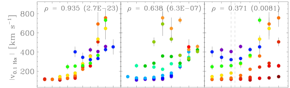
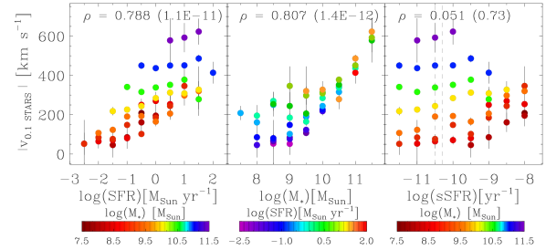
Figure 15: (Modulus of the) 0.1th percentile velocity of the LoSVD of the ionised gas as traced by the [OIII] (top panel) and H$\alpha$ (middle panel) emission lines, and of the stars (bottom panel). For a Gaussian velocity distribution, the 0.1th percentile velocity corresponds to -3 standard deviations ($\sigma$) from the mean velocity, and therefore it probes the high velocity blueshifted tail of the LoSVD. Similarly to Fig. 14, we report for each plot the Spearman rank correlation coefficient $\rho$ along with its associated two-sided p-value.

To this purpose, we calculate the 0.1th, 2.3th,15.9th, 84.1th, 97.7th and 99.9th percentile velocities of the LoSVDs of gas and stars. We chose these values because, in a Gaussian distribution, they correspond respectively to $-3\sigma$, $-2\sigma$, $-1\sigma$, $1\sigma$, $2\sigma$ and $3\sigma$, where $\sigma$ is the standard deviation of the Gaussian distribution. The $N$-th percentile velocity, $v_{N}$, is defined as:

$$P(v<v_{N})=\int_{-\infty}^{v_{N}}\mathcal{L}(v)dv=N,$$ (7)

where $P(v<v_{N})$ is the probability of observing, with the given line-of-sight velocity distribution $\mathcal{L}(v)$, velocities lower than $v_{N}$, and ${\int_{-\infty}^{+\infty}\mathcal{L}(v)dv=1}$.

Figure 15 shows the 0.1th percentile velocities of the [OIII], H$\alpha$ and stellar LoSVDs as a function of SFR, M_∗ and sSFR. The corresponding plots obtained for the other percentile velocities are shown in the Appendix (Figures 22 to  26). The results of the Spearman rank test performed on the relationships between the various LoSVD parameters ($\sigma$ and percentile velocities) and galaxy parameters (SFR, M_∗ and sSFR), for both gas and stars, are reported in Table 1 to facilitate the comparison between the different relationships shown in Figs. 14, 15 and 22–26.

Table 1: Spearman rank correlation parameters^†

	[OIII]	H$\alpha$	stars
	$\rho$ (p-value)	$\rho$ (p-value)	$\rho$ (p-value)
$\sigma$ vs SFR	0.906 (1.5E-19)	0.918 (7.5E-21)	0.795 (5.4E-12)
$v_{15.9}$ vs SFR	0.826 (1.6E-13)	0.852 (4.4E-15)	0.825 (1.7E-13)
$v_{2.3}$ vs SFR	0.891 (4.7E-18)	0.925 (8.5E-22)	0.792 (7.3E-12)
$v_{0.1}$ vs SFR	0.938 (8.9E-24)	0.935 (2.7E-23)	0.788 (1.1E-11)
$v_{84.1}$ vs SFR	0.760 (1.5E-10)	0.735 (1.2E-09)	0.787 (1.3E-11)
$v_{97.7}$ vs SFR	0.889 (6.5E-18)	0.885 (1.6E-17)	0.756 (2.3E-10)
$v_{99.9}$ vs SFR	0.921 (2.5E-21)	0.894 (2.2E-18)	0.731 (1.7E-09)
$\sigma$ vs M∗	0.810 (9.9E-13)	0.752 (3.0E-10)	0.810 (1.1E-12)
$v_{15.9}$ vs M∗	0.832 (7.0E-14)	0.790 (9.4E-12)	0.802 (2.7E-12)
$v_{2.3}$ vs M∗	0.808 (1.3E-12)	0.730 (1.8E-09)	0.808 (1.3E-12)
$v_{0.1}$ vs M∗	0.678 (6.2E-08)	0.638 (6.3E-07)	0.807 (1.4E-12)
$v_{84.1}$ vs M∗	0.886 (1.3E-17)	0.820 (3.4E-13)	0.792 (7.3E-12)
$v_{97.7}$ vs M∗	0.810 (1.1E-12)	0.754 (2.5E-10)	0.815 (6.2E-13)
$v_{99.9}$ vs M∗	0.566 (1.9E-05)	0.657 (2.2E-07)	0.811 (8.8E-13)
$\sigma$ vs sSFR	0.175 (0.22)	0.246 (0.085)	0.059 (0.69)
$v_{15.9}$ vs sSFR	0.069 (0.64)	0.142 (0.33)	0.094 (0.52)
$v_{2.3}$ vs sSFR	0.159 (0.27)	0.268 (0.059)	0.054 (0.71)
$v_{0.1}$ vs sSFR	0.332 (0.019)	0.371 (0.0081)	0.051 (0.73)
$v_{84.1}$ vs sSFR	-0.044 (0.76)	-0.002 (0.99)	0.070 (0.63)
$v_{97.7}$ vs sSFR	0.160 (0.27)	0.207 (0.15)	0.019 (0.90)
$v_{99.9}$ vs sSFR	0.435 (0.0016)	0.314 (0.026)	-0.005 (0.97)

Notes: ^† This table lists the Spearman rank correlation coefficients ($\rho\in(0.1)$) and corresponding two-sided p-values calculated for the relationships between LoSVD parameters (velocity dispersion and percentile velocities) and galaxy properties (SFR, M_∗, sSFR) that are shown in Figs. 14, 15 and Figs.  22–26. A high value of $\rho$ (e.g. $\rho\gtrsim 0.5$) combined with a low p-value ($\leq 0.05$) indicates the presence of a statistically significant correlation.

It is clear from Table 1 that the velocity dispersions and the percentile velocities show all significant correlations with SFR and M_∗, for both the gas and the stars. There are however important differences among the various LoSVD parameters, in particular between the 15.9th and the 0.1th percentile velocities. More specifically, by moving towards the high velocity blueshifted tail of the LoSVD (i.e. from the 15.9th to the 0.1th percentile velocity), the correlation between gas velocity and SFR tightens (the Spearman correlation coefficient $\rho$ increases), whereas the correlation between stellar velocity and SFR weakens slightly ($\rho$ decreases). A similar trend is evidenced also for the redshifted tail of the LoSVD (i.e. from the 84.1th to the 99.9th percentile velocity). These results strengthen the hypothesis that the high velocity tail of the ionised gas LoSVD traces mainly star formation-feedback related mechanisms and is little affected by other mechanisms, which instead dominate the relationships between stellar velocity and SFR. The correlation between gas velocity and SFR is slightly tighter at blueshifted than at redshifted velocities (especially if using H$\alpha$ as a tracer), probably because of dust extinction affecting mostly the receding (i.e. redshifted) side of the outflow. Furthermore, Table 1 shows that the correlation between ionised gas velocity and M_∗ weakens (and almost breaks down, as clearly shown in the corresponding plots in Fig. 15 and Figs. 24–26) towards the high velocity tail of the LoSVD ($\rho$ decreases), suggesting that gravity (as traced by M_∗) does not play an important role in determining the dynamics of the high-velocity gas.

In summary, by exploring the relationships between the different percentile velocities of the LoSVDs of gas and stars and the galaxy parameters, we infer that the correlation with the SFR is tighter for the ionised gas at higher percentile velocities and, in particular, that the high velocity (blueshifted or redshifted) tails of the gaseous LoSVDs depend tightly on the SFR (correlation coefficient $\rho\gtrsim 0.9$) and more weakly ($\rho<0.7$) on the stellar mass. This result supports the hypothesis that, in the high velocity regime, the gas kinematics progressively ceases to probe the dynamical mass of galaxies (which is in first approximation traced by the stellar mass), but it is instead intrinsically related to the rate at which stars are formed, likely because of the presence of stellar feedback mechanisms.

However, regardless of the correlations observed between the various LoSVD parameters ($\sigma$ and percentile velocities) and galaxy properties (SFR, M_∗, sSFR) that have been discussed in this Section (Table 1), in order to isolate the effects of outflows from other mechanisms we need to investigate the differences between the LoSVDs of gas and stars. Indeed, by looking at the galaxy stacks where the difference $(v_{\rm gas}-v_{\rm stars})$ is significantly greater than zero, we can identify galaxies where the motions of gas and stars are clearly decoupled, and so galaxies where outflows are most likely taking place. Differences between the gaseous and stellar kinematics and their dependency on galaxy properties will be investigated in $\S$ 3.4.

3.3 Asymmetries in the LoSVDs of gas and stars

Asymmetric wings of nebular emission lines usually trace perturbed gas, whose dynamics is not consistent with purely virial motions but that can be instead explained with radial (outward or inward) motions in conjunction with dust extinction effects. The presence of a blue asymmetry is commonly interpreted in terms of outflows, because obscuration by dust in the galaxy disk affects primarily the backside receding gas (e.g. Lehnert & Heckman 1996; Villar-Martín et al. 2011; Soto et al. 2012).

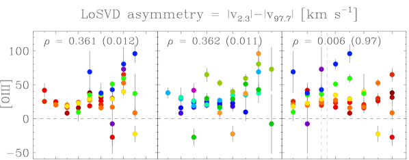
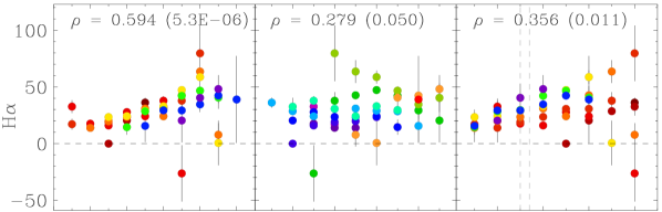
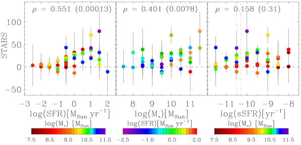
Figure 16: Blue asymmetry of the [OIII] (top panel), H$\alpha$ (middle panel) and stellar (bottom panel) LoSVDs, as measured by the difference between the (moduli of the) 2.3th and 97.7th percentile velocities (i.e. $y=|v_{2.3}|-|v_{97.7}|$). For display purposes, only the less noisy bins are plotted, i.e. bins with either $\sigma_{y}<50\leavevmode\nobreak\ {\rm km\leavevmode\nobreak\ s^{-1}}$ or $|y|\geq 2\sigma_{y}$. The Spearman rank correlation coefficient ($0<\rho<1$, higher values of $\rho$ indicate stronger correlation) is reported for each plot, along with the corresponding two-sided p-value (if the p-value is $\leq\alpha$, where $\alpha=0.05$ is the level of significance, the observed correlation is statistically significant).

Visual inspection of the LoSVD profiles of gas and stars shown in Figs. 8 to 13 suggests that the line-of-sight velocity distributions of both gas and stars are not symmetrical. We further investigate this possibility in Fig. 16, where we plot, as a function of SFR, M_∗ and sSFR, the difference between the (moduli of the) 2.3th and 97.7th percentile velocities, i.e. ${|v_{2.3}|-|v_{97.7}|}$, evaluated for [OIII], H$\alpha$ and stars. Figure 16 shows that almost all galaxy bins (a part form a few, noisier stacks) exhibit a clear blue asymmetry in the LoSVDs of [OIII] and H$\alpha$, with ${|v_{2.3}|-|v_{97.7}|}$ values ranging between $\sim 0$ km s^-1 and $\sim 100$ km s^-1. Very surprisingly, also the stellar LoSVDs are affected by a blueward asymmetry, although less pronounced than in the gas. The velocity difference ${|v_{2.3}|-|v_{97.7}|}$ measured for the stars is consistent with zero at low SFRs. However, in galaxy bins with ${\rm SFR\gtrsim 0.1\leavevmode\nobreak\ M_{\odot}\leavevmode\nobreak\ yr^{-1}}$, ${|v_{2.3}|-|v_{97.7}|}$ increases up to values of a few tens of km s^-1, with large uncertainties, but still significantly larger than zero and therefore inconsistent with the absence of any asymmetry.

The presence of a blue asymmetry in the LoSVDs of [OIII] and H$\alpha$ is suggestive of galactic outflows. The hypothesis of star formation-driven outflows is corroborated by the correlation observed between the H$\alpha$ blue asymmetry (as traced by ${|v_{2.3}|-|v_{97.7}|}$) and the SFR ($\rho$=0.594), and by the hint of a correlation observed for [OIII] ($\rho$=0.361). We note however that the dust properties of galaxies may also affect the trends observed for [OIII] and H$\alpha$ in Fig. 16. Indeed Santini et al. (2014), by using Herschel observations of local and intermediate-redshift ($z\lesssim 2.5$) galaxies, found a tight correlation between dust mass and star formation rate, which they interpreted as a consequence of the Schmidt–Kennicutt law (since dust and gas mass are related). Therefore, the positive correlation between ${|v_{2.3}|-|v_{97.7}|}$ and SFR observed for the ionised gas is likely due to the combined effect of star formation-driven outflows and ${\rm M_{dust}}$–SFR proportionality, since dustier galaxy disks result in more pronounced line asymmetries. The evidence for a relationship between LoSVD blue asymmetry and stellar mass is instead more marginal ($\rho=0.362$ and $\rho=0.279$, respectively for [OIII] and H$\alpha$, second column of Fig. 16). The absence of a clear correlation is consistent with the recent results by Santini et al. (2014), who showed that the positive correlation between dust and stellar mass found by previous studies significantly flattens when separating galaxies according to their SFR.

Figure 16 shows that, in the stellar LoSVDs, blue asymmetries are also present but, due to the large uncertainties, it is very difficult to investigate possible relationships with galaxy properties. However, we note that there is some evidence for a weak correlation between stellar blue asymmetry and SFR ($\rho=0.551$), and an even more marginal one with stellar mass ($\rho=0.401$), vaguely recalling the corresponding trends observed in ionised gas.

In Figure 5 ($\S$ 2.5) we showed a check on the stellar continuum fitting for two galaxy stacks: one exhibiting a blue asymmetry in the stellar LoSVD, and one with no asymmetry. These plots demonstrate that the detection of such a faint feature in the stellar kinematics of external galaxies is made possible thanks to the high signal-to-noise reached in the composite spectra, which allows us to fit the stellar continuum (and so extract the stellar kinematics) with unprecedented accuracy. To our knowledge, blue asymmetries in the stellar LoSVDs of external galaxies have never been observed before. Indeed, while an intrinsic kinematic asymmetry or “lopsidedness” in the stellar distribution is certainly possible for individual galaxies or at specific locations within galaxies, for example due to stellar bars, galaxy interactions or even counter-rotating disks (e.g. Krajnović et al. 2015), such effects should average out when combining the integrated spectra of thousands of different galaxies. The observation of an asymmetry of the stellar LoSVD that is consistently blue (and never red) could be explained by the presence of stars in radial outward motions in galaxies, combined with obscuration by dust lanes in the galactic disk. Dust in the disk would hamper mainly the detection of stars moving away from the galaxy with a redshifted (line-of-sight) velocity component, hence skewing the average stellar LoSVD towards blueshifted velocities.

The blue asymmetries in the stellar LoSVDs suggest that high-velocity runaway stars, hypervelocity stars (HVS, Brown et al. (2005)) and possibly high-velocity stellar clusters (Caldwell et al., 2014) in radial motions may be a rather common phenomenon in star forming galaxies. High velocity stars in radial trajectories are usually very difficult to detect even in our own galaxy. Palladino et al. (2014) discovered a sample of 20 candidate hypervelocity stars in the Milky Way, the bulk of which have velocities between 600 and 800 km s^-1, and in at least half of the cases exceed the escape velocity from the Galaxy. These are G- and K-type dwarf stars, hence less massive and older than the typical massive B-type HVSs (Brown et al., 2012). Interestingly, the trajectories of the stars detected by Palladino et al. (2014) are not consistent with ejection via three-body interactions between a binary system and the SMBH of our Galaxy or of M31, which is currently the most popular explanation for young B-type hypervelocity stars (Hills, 1988; Yu & Tremaine, 2003) and predicts that one component of the binary system remains in a bound orbit around the SMBH. On the contrary, the HVS candidates detected by Palladino et al. (2014) appear to originate from all directions, suggesting that another mechanism must be capable of accelerating stars to high speeds, such as a supernova explosion in a close binary system (Blaauw, 1961; Zubovas et al., 2013), which is currently the most likely origin of lower speed runaways ejected from the galactic disk (Brown et al., 2015). Notably, the fastest HVS ever detected, US 708, with a Galactic rest-frame velocity of 1200 km s^-1, has been recently confirmed to be a solid candidate for an ejected Type Ia supernova donor remnant (Geier et al., 2015). The supernova binary ejection scenario may be a viable explanation for our observations, supported by the tentative correlation observed in Fig. 16 between the stellar blue asymmetry and the SFR.

However, although HVSs may provide a plausible explanation for the blue asymmetries observed in the stellar LoSVDs of local star forming galaxies, the properties and origin of these features need further and in-depth investigation with high signal-to-noise data such as will be delivered by ongoing surveys (Gaia, MaNGA) and new facilities (MUSE, JWST, 30m class telescopes).

3.4 Outflow properties

Overall, the presence and properties of the line-of-sight velocity distributions of ionised gas as derived from composite spectra of nearby non-active galaxies suggest ubiquity of star formation-driven galactic outflows. However, our analysis has also highlighted the presence of additional factors, other than outflows, that are likely affecting the kinematics of both the ionised gas and the stars, namely virial motions, projection effects, gas content, and dust extinction. The next step is to try to isolate in the data the effects of gas outflows, disentangling them from other mechanisms, in order to get a completely unbiased picture of their occurrence and properties in local galaxies.

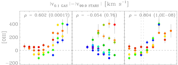
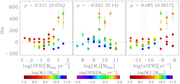
Figure 17: Excess of line-of-sight velocity of the ionised gas with respect to the stars ($v_{\rm gas}-v_{\rm stars}$) as given by $y=|v_{\rm 0.1\leavevmode\nobreak\ gas}|-|v_{\rm 99.9\leavevmode\nobreak\ stars}|$ for [OIII] (upper panel) and for H$\alpha$ (bottom panel). For display purposes, only the less noisy bins are plotted, i.e. only bins with either $\sigma_{y}<{\rm 50\leavevmode\nobreak\ km\leavevmode\nobreak\ s^{-1}}$ or $|y|\geq 2\sigma_{y}$. As explained in $\S$ 3.4, the quantity $y$ is a reliable tracer of ionised outflows only when it is positive. The Spearman rank correlation coefficient ($0<|\rho|<1$, higher values of $|\rho|$ indicate stronger correlation, $\rho<0$ if there is an anti-correlation) is reported in each plot, along with the corresponding two-sided p-value (if the p-value is $\leq\alpha$, where $\alpha=0.05$ is the level of significance, the observed correlation is statistically significant).

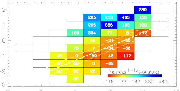
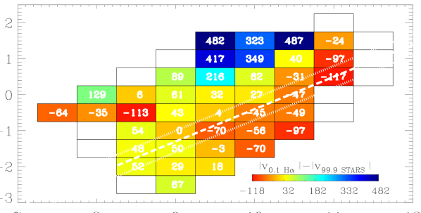
Figure 18: Grid of galaxy bins in the M_∗–SFR parameter space used for the spectral stacking (see also Fig. 1). Each bin is colour-coded according to the line-of-sight velocity difference $v_{\rm gas}-v_{\rm stars}$ as given by $|v_{\rm 0.1\leavevmode\nobreak\ gas}|-|v_{\rm 99.9\leavevmode\nobreak\ stars}|$ for [OIII] (upper panel) and for H$\alpha$ (lower panel). The $|v_{\rm 0.1\leavevmode\nobreak\ gas}|-|v_{\rm 99.9\leavevmode\nobreak\ stars}|$ values are also reported for each bin. The same bins as in Fig. 17 are plotted.

The plots in Figs. 14,  15 and 16 provided important clues on the concomitant mechanisms that have an impact on the LoSVDs of gas and stars. In the following, we briefly summarise some logical deductions that will help us understand outflow properties:

1. The effects of virial motions on gas kinematics can be reduced considerably by looking at the high velocity tail of the LoSVD of the ionised gas. In particular, the correlation between the line-of-sight velocity of the ionised gas and M_∗ (which is related to the dynamical mass) is weaker for the 0.1th and 99.9th ($\rho\sim 0.6$) than for the 15.9th and 84.1th ($\rho\sim 0.8$) percentile velocities (Table 1). Moreover, the highest velocities show the tightest correlation with the SFR ($\rho\gtrsim 0.9$), indicating that the effects of star formation-driven feedback is indeed predominant.

2. The stellar LoSVDs appear quite broad, with stellar velocity dispersions as high as $\sim 170$ km s^-1, i.e. as high as the highest $\sigma$ observed in the ionised gas and, for large stellar masses, even higher than the gas, probably because of the presence of stellar bulges in massive galaxies combined with projection effects, as explained in $\S$ 3.2. As a consequence, only the excess of gas velocity with respect to the stars, i.e. $v_{\rm gas}-v_{\rm stars}$, can reliably trace gas motions due to gaseous outflows.

3. Because of dust attenuation, the blueshifted side of the LoSVD of the gas is a better probe of outflowing gas than the redshifted side. Therefore, following points (i) and (ii), gaseous outflows will be investigated through the 0.1th percentile velocity of the LoSVD of [OIII] and H$\alpha$, from which we will subtract the corresponding stellar velocity.

4. Another complication for the study of ionised outflows is given by the presence of (modest) blue asymmetries in the stellar LoSVDs, whose origin is not clear and may be related to non virial motions of stars in galaxies. In the following analysis we will assume that this effect can be reduced (if not completely removed) by simply using the redshifted stellar velocities, i.e. by subtracting from the 0.1th percentile LoS velocity of the gas, the 99.9th (rather than the 0.1th) percentile LoS velocity of the stars.

By considering points 1 to 4, the most appropriate tracer of ionised outflows is then given by the velocity difference $|v_{\rm 0.1\leavevmode\nobreak\ gas}|-|v_{\rm 99.9\leavevmode\nobreak\ stars}|$: this quantity will be used to track “secure” outflows in galaxy stacks. Indeed, if $(v_{\rm gas}-v_{\rm stars})>0$, then the kinematics of gas and stars are decoupled and we are reliably tracing gaseous outflows. The only other mechanism that would explain such decoupling would be galaxy mergers, but the merger fraction is negligible in the local Universe (Patton & Atfield, 2008), so gaseous outflows are the only viable explanation.

Figure 17 shows the relationships between the quantity $|v_{\rm 0.1\leavevmode\nobreak\ gas}|-|v_{\rm 99.9\leavevmode\nobreak\ stars}|$, evaluated for both [OIII]- and H$\alpha$-emitting gas, and the galaxy physical parameters (i.e. SFR, ${\rm M_{*}}$ and sSFR). In Fig. 18 we show the stacking grid in the M_∗–SFR parameter space defined by the sample of local star forming galaxies used in this study (i.e. the same grid as Fig. 1), with each bin colour-coded according to the value of $|v_{\rm 0.1\leavevmode\nobreak\ gas}|-|v_{\rm 99.9\leavevmode\nobreak\ stars}|$ (measured for [OIII] and H$\alpha$).

It is worth emphasising that the negative values of $|v_{\rm 0.1\leavevmode\nobreak\ gas}|-|v_{\rm 99.9\leavevmode\nobreak\ stars}|$ estimated in some galaxy bins (especially at ${\rm log(M_{*}[M_{\odot}])\geq 10.0}$), are probably a consequence of the conjunction of projection effects and of the absence of detectable galactic outflows. More specifically, ignoring galactic outflows (which usually expand out perpendicular to the galactic disk, along its minor axis, as shown by observations, e.g. Lehnert & Heckman 1996; Heckman et al. 2000; Chen et al. 2010; Rubin et al. 2014; Cazzoli et al. 2014), the ionised gas is confined to the plane of the galactic disk, and the projection effects described in $\S$ 3.2, affecting mostly observations of face-on galaxies with a prominent stellar bulge (which dominate the population of high-M_∗ galaxies, e.g. Gavazzi et al. 2015), can be even more accentuated. For this reason, negative values of $|v_{\rm 0.1\leavevmode\nobreak\ gas}|-|v_{\rm 99.9\leavevmode\nobreak\ stars}|$ simply indicate galaxy bins in which outflows are not present, or in which outflows are not prominent enough to be detected: as a consequence, this quantity can reliably trace outflows only when it is positive.

Although many attempts have been made to establish fundamental “scaling” relationships linking outflows and galaxy properties (Martin, 2005; Rupke et al., 2005; Chen et al., 2010; Westmoquette et al., 2012; Martin et al., 2012; Rubin et al., 2014; Arribas et al., 2014; Heckman et al., 2015), the general picture remains unclear and contradictory. The main reason for this impasse may be the absence of a study on galactic outflows of large statistical significance: most of previous studies relied on limited samples of objects, showing extreme characteristics and spanning only a narrow range of galaxy properties (e.g. SFR, M_∗). As a consequence, previous results do not adequately represent the whole local population of galaxies. Our analysis instead capitalises on a large statistical and almost unbiased sample of local star forming galaxies, particularly suitable for determining scaling relationships between galactic outflows and galaxy properties. Moreover, our method allows, to accurately identify and separate of the effects of star-formation driven outflows from the other mechanisms affecting the LoSVD of the gas.

The general picture emerging from Figs. 17 and 18 is the following: the excess of gas velocity with respect to the stars (i.e. $v_{\rm gas}-v_{\rm stars}$, as traced by $|v_{\rm 0.1\leavevmode\nobreak\ gas}|-|v_{\rm 99.9\leavevmode\nobreak\ stars}|$), which we use in this study to trace galactic outflows, depends weakly on the SFR ($\rho=0.602$ for [OIII], but for H$\alpha$ the correlation with SFR is much weaker, $\rho=0.311$, and not statistically significant as indicated by the high p-value) and more tightly on the sSFR ($\rho=0.804$ and $\rho=0.485$ for [OIII] and H$\alpha$ respectively). However, we note that for galaxy bins identified by higher stellar masses the correlation between $|v_{\rm 0.1\leavevmode\nobreak\ gas}|-|v_{\rm 99.9\leavevmode\nobreak\ stars}|$ and SFR at a fixed M_∗ becomes significantly tighter for both [OIII] and H$\alpha$, i.e. $\rho>0.8$ (with $\rm p-value\ll 0.05$) at M${}_{*}\geq 10^{9.5}$ M_⊙ and even more so at M${}_{*}\geq 10^{10}$ M_⊙, for which we measure $\rho>0.95$.

Globally, there is instead no relation between $|v_{\rm 0.1\leavevmode\nobreak\ gas}|-|v_{\rm 99.9\leavevmode\nobreak\ stars}|$ and M_∗ (second column of Fig. 17): $\rho=-0.054$ for [OIII] and $\rho=-0.242$ for H$\alpha$, but with high p-values, implying that such weak anti-correlation is not significant. For some galaxy bins, an anti-correlation appears between $|v_{\rm 0.1\leavevmode\nobreak\ gas}|-|v_{\rm 99.9\leavevmode\nobreak\ stars}|$ and M_∗ at a fixed SFR. This effect is however highly significant ($\rho<-0.9$) for both [OIII] and H$\alpha$ only at $\rm log(SFR[M_{\odot}\leavevmode\nobreak\ yr^{-1}])=-1.0$ and $\rm log(SFR[M_{\odot}\leavevmode\nobreak\ yr^{-1}])=0.5$. Since the stellar mass traces the depth of the gravitational potential in galaxies, these observations would suggest that, on equal SFRs, it becomes increasingly difficult to launch gaseous outflows in larger gravitational potentials by means of star formation feedback only. This qualitatively agrees with theoretical predictions (further discussed in $\S$ 4.1) as well as with indirect observational evidence for a mass dependance of negative feedback provided by studies of the “mass-metallicity” relationship in galaxies (Tremonti et al., 2004; Maiolino et al., 2008). These studies showed that the gas-phase metallicity increases steadily with stellar mass, at least up to ${\rm log(M_{*}[M_{\odot}])\simeq 10.5}$, suggesting that low mass galaxies are less able than massive galaxies to retain in their gas phase the metals provided by supernova explosions, probably because they are more vulnerable to galactic outflows.

In addition, Fig. 17 reveals some interesting differences between [OIII] and H$\alpha$ as tracers of ionised outflows. In particular, H$\alpha$ emission seems to be a worse tracer of galactic outflows than [OIII] emission: (i) The correlation between $v_{\rm gas}-v_{\rm stars}$ and SFR is considerably weaker and less significant for H$\alpha$ than for [OIII], and the same holds for the correlation with sSFR; (ii) for bins with $\rm log(M_{*}[M_{\odot}])=11.0$, high values of $|v_{\rm 0.1\leavevmode\nobreak\ gas}|-|v_{\rm 99.9\leavevmode\nobreak\ stars}|$ are inferred by using [OIII], whereas no velocity excess is detected when using H$\alpha$ emission as a gas tracer. Qualitatively, an higher outflow ionisation in more massive galaxies could explain the differences that we evidence between [OIII] and H$\alpha$ as outflow tracers. We note that it is unlikely that such a difference between the H$\alpha$ and [OIII] LoSVDs is a consequence of residual stellar H$\alpha$ absorption. Indeed, the H$\alpha$ LoSVDs are obtained by fitting the H$\alpha$ and [NII]$\lambda\lambda$6548,6583 lines simultaneously (see $\S$ 2.6), by constraining the kinematics of all components employed in the fit to be the same for the three lines. Therefore, the resulting LoSVDs reflect also the kinematics traced by the [NII] lines, which are much less affected by possible residual stellar absorption.

Finally, we note that there is an intriguing property of galactic outflows that stands out immediately from Fig. 18: local non-active galaxies hosting powerful outflows are located above the main sequence of star forming galaxies. The absence (or insignificance) of galactic outflows along and/or below the MS, which we show here for the first time in a clear way, probably constitutes a striking feature of the local galaxy population, and it may persist to higher redshifts, as marginally shown in outflow studies at $z\sim 1$ (Martin et al., 2012). The relationship between galactic outflows and the MS of star forming galaxies will be further discussed in $\S$ 4.2.

4 Discussion

4.1 Implications of outflow properties for feedback models

Intense star formation activity conveys energy and momentum to its surroundings, which can then be transmitted by various physical mechanisms to larger scales, thus eventually impacting the entire host galaxy and affecting its capability of forming stars (negative feedback). Although negative feedback from star formation can manifest under various forms (such as galactic outflows of ionised, neutral and molecular gas, shocks, hot bubbles and cavities, metal-enrichment of the IGM), its direct and unambiguous signature can be very difficult to detect in most galaxies. As a consequence, the detailed physics underlying this phenomenon is not yet completely understood, as well as its relevance for quenching star formation in galaxies. However, significant advances have been accomplished by theorists in this field, who, by also exploiting the valuable information provided by observational studies, propose two main scenarios for star formation-driven feedback to occur:

1. According to the first,“canonical” scenario, the kinetic energy released by supernova explosions and, especially in the very first stages of the starburst ($\Delta t\leq 10^{7}\rm yrs$) and at high metallicities ($\mathcal{Z}\geq\mathcal{Z}_{\odot}$), by stellar winds from OB and Wolf-Rayet stars, plays the most important role in counteracting and self-regulating star formation ( “energy-driven” scenario, e.g. Chevalier 1977; Leitherer et al. 1992; Chevalier & Clegg 1985; Springel & Hernquist 2003; Veilleux et al. 2005). This feedback mechanism is subject to the thermalisation efficiency of the energy deposited into the ISM: such efficiency may vary, but it is believed to be around 1-10%; therefore, up to $\sim$99% of the total kinetic energy injected by star formation may be dissipated radiatively in dense gas (Chevalier, 1977; Murray et al., 2005; Thornton et al., 1998; Mac Low & Ferrara, 1999). If the transfer from kinetic energy from SNe and stellar winds to cloud motions is efficient enough to unbind the gas in the galaxy, it can drive strong and large-scale outflows (Chevalier & Clegg, 1985). A natural outcome of this model is that energy-driven outflows are more important, at a given SFR (which is directly related to the kinetic energy injected by supernova ejecta and by stellar winds into the ISM), in low mass galaxies residing in less massive dark matter halos, because it is easier for gas to escape from their shallower gravitational wells (Dekel & Silk, 1986; Springel & Hernquist, 2003; Davé et al., 2011b).

2. In the second scenario, the momentum transferred by the UV radiation from young and massive stars to dust and the momentum injected by supernova explosions (“momentum-driven” scenario) dominate the feedback mechanism (Murray et al., 2005; Davé et al., 2011b). The advantage of momentum-driven outflows is that they can be effective even when radiative losses are high, because momentum cannot be radiated away (Murray et al., 2005). However, this feedback mechanism, in order to be effective, requires ISM conditions that may not be satisfied in normal local star-forming galaxies, such as large optical depths to infrared radiation (Davé et al., 2011b; Hopkins et al., 2011), as well as collisional coupling of gas and dust in the outflow (Murray et al., 2005; Davé et al., 2011b). For these reasons, momentum-driven outflows may be most effective at launching cold and dense gas (which is likely hydrodynamically coupled to dust) in dusty star-forming galaxies and AGNs (Murray et al., 2005; Fabian, 2012). We note that in this model, according to the original formulation by Murray et al. (2005), the condition that must be satisfied in order to launch gas outward via momentum injection is that the total momentum flux exceeds the gravitational force, which translates into a condition on the luminosity of the starburst $L\geq L_{M}$, where $L_{M}$ is an “Eddington-like” luminosity threshold. If $L\geq L_{M}$, a momentum-driven wind develops, with velocity $v_{\rm out}\gtrsim 2\sigma_{*}$ (where $\sigma_{*}$ is the stellar velocity dispersion; Murray et al. 2005).

In $\S$ 3.4 we have identified the galaxy stacks displaying the signature of galactic outflows as those for which the excess of gas velocity with respect to the stellar velocity, as estimated from the high-velocity tail of the LoSVD, is significant. More specifically, we have considered values of ${|v_{\rm 0.1\leavevmode\nobreak\ gas}|-|v_{\rm 99.9\leavevmode\nobreak\ stars}|}$ significantly greater than zero as a clear signature of outflows. The next step would be comparing the scaling relationships obtained for the observed outflows with the expectations of theoretical models. However, the quantity ${|v_{\rm 0.1\leavevmode\nobreak\ gas}|-|v_{\rm 99.9\leavevmode\nobreak\ stars}|}$, while being suitable for identifying outflows, is not appropriate for the comparison with models, because it has no clear interpretation in terms of the physical quantities usually employed by theorists. Unfortunately, because of the information lost with the stacking, it is not possible to estimate the mass entrained in the observed outflows, and therefore to calculate some important parameters such as mass-loss rate, kinetic power and momentum rate of the outflows, which would help to discriminate between different feedback models. Most importantly, spatially resolved spectroscopic information are needed to infer these quantities (Rupke & Veilleux, 2013; Cazzoli et al., 2014; Arribas et al., 2014). However, we can obtain a proxy of the outflow velocity, and this can be exploited to shed light on the physical mechanism powering the ionised outflows.

The LoSVD of ionised gas traces a combination of dynamical motions of gas clouds within the gravitational potential of the galaxy and of perturbed motions due to star formation feeedback-related processes such as outflows and turbulence in the disk. In the following analysis, since we consider only the high-velocity tail of the LoSVD, we assume that outflows dominate over turbulence, and so, simplistically, that any non-gravitational motions of the gas at such high velocities are due to outflows and not to turbulence. Therefore, the LoSVD of the gas may be regarded as the convolution of two line-of-sight velocity distributions, one tracing the virial motions, and the other one tracing the outflow:

$$\mathcal{L}_{\rm gas}(v)=\mathcal{L}_{\rm virial}(v)\ast\mathcal{L}_{\rm outflow}(v).$$ (8)

We note that such approximation reflects the fact that the typical outflows detected in our galaxy sample are rather modest, and most likely consist of localised bubbles and chimneys, emanating from star forming regions spread across the stellar disk (see also the case of NGC 1569 discussed by Martin et al. 2002). In this scenario, the outflowing material participates, at least to some extent, also to the virial (rotational) motions in the galaxy. However, we stress that Eq. 8 is not universally applicable. In particular, Eq. 8 does not hold if the kinematics of the high velocity gas is largely dominated by a large-scale “bulk outflow” expanding perpendicular to the disk. This is the case of powerful starburst-driven superwinds (e.g. M 82, NGC 253) if they are probed on scales of at least a few kpc, i.e. sufficiently larger than the typical vertical scale height of the stellar disk, where the motions of the gas in outflow is clearly distinct from the disk motions. Indeed, even the strong “bulk outflows” that develop in powerful starbursts such as M 82 appear to originate as a collection of individual chimneys expanding out from the disk that subsequently merge to form the classical biconical outflows observed on kpc scales (Wills et al., 1999; Lehnert & Heckman, 1996).

Following from Eq. 8, by (simplistically) approximating both $\mathcal{L}_{\rm virial}(v)$ and $\mathcal{L}_{\rm outflow}(v)$ with Gaussian distributions, the line-of-sight velocity dispersion of the gas corresponds to:

$$\sigma_{\rm gas}^{2}=\sigma_{\rm virial}^{2}+\sigma_{\rm outflow}^{2},$$ (9)

where $\sigma_{\rm virial}$ can be approximated by the stellar line-of-sight velocity dispersion, i.e. $\sigma_{\rm virial}\approx\sigma_{\rm stars}$. As a result, the “outflow” line-of-sight velocity dispersion would be:

$$\sigma_{\rm outflow}=(\sigma_{\rm gas}^{2}-\sigma_{\rm stars}^{2})^{1/2}.$$ (10)

We note that Eq. 10 can be extended also to the percentile velocities as, in the approximation of Gaussian distributions, they correspond to multiples of the velocity dispersion. Therefore, according to this line of reasoning, the outflow velocity can be approximated by the quantity $(v_{N,{\rm gas}}^{2}-v_{N,{\rm stars}}^{2})^{1/2}$, where $v_{N}$ indicates the $N$-th percentile velocity.

As we commented earlier, because of the observed blue asymmetries observed in the stellar LoSVDs of some galaxy stacks ($\S$ 3.3), the percentile velocities on the blue side of the stellar LoSVD, i.e. the 15.9th, 2.3th and 0.1th, may be not appropriate to trace virial motions in the galaxy. Therefore, in the following, we adopt the same strategy as in $\S$ 3.4 and define the outflow velocity as:

$$v_{\rm out}=(v_{N,{\rm gas}}^{2}-v_{100-N,{\rm stars}}^{2})^{1/2},$$ (11)

where the percentile velocity of the gas is chosen on the blue side of the LoSVD (because it is less affected by dust), i.e. $N$= 0.1, 2.3 or 15.9, and, for the stars, we use $100-N$, which gives the corresponding percentile velocity on the red side of the LoSVD. We note that $v_{\rm out}$ can be inferred from Eq. 11 only in those cases for which $v_{N,{\rm gas}}>v_{100-N,{\rm stars}}$: this means that $v_{\rm out}$ cannot be calculated for quite a few bins below the MS, as illustrated by Fig. 18.

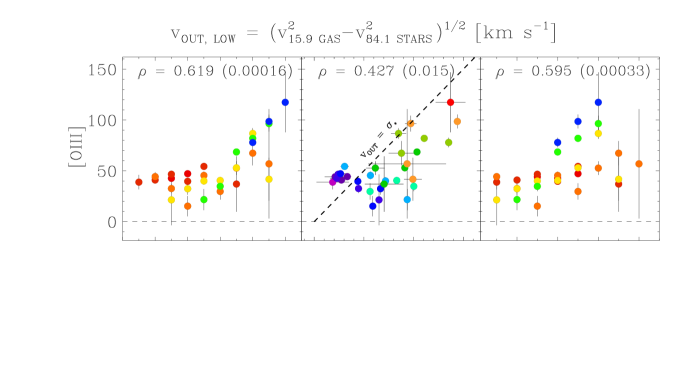
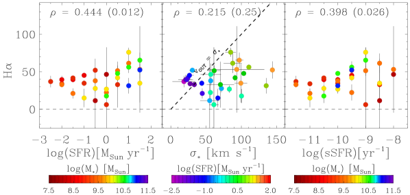
Figure 19: Outflow velocity as given by $(v_{\rm 15.9\leavevmode\nobreak\ gas}^{2}-v_{\rm 84.1\leavevmode\nobreak\ stars}^{2})^{1/2}$ (see explanation in $\S$ 4.1) inferred from [OIII] (upper panel) and H$\alpha$ emission (bottom panel), plotted as a function of SFR, stellar velocity dispersion (as obtained from the fit to the stellar continuum), and sSFR. The same bins as Fig. 17 are plotted, excluding those for which $(v_{\rm 15.9\leavevmode\nobreak\ gas}^{2}-v_{\rm 84.1\leavevmode\nobreak\ stars}^{2})<0$. In the middle panels, the dashed lines indicate the locus of points where $v_{\rm out}=\sigma_{\rm stars}$. The Spearman rank correlation coefficient ($0<\rho<1$, higher values of $\rho$ indicate stronger correlation) is reported for each plot, along with the corresponding two-sided p-value (if the p-value is $\leq\alpha$, where $\alpha=0.05$ is the level of significance, the observed correlation is statistically significant).

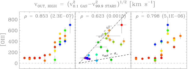
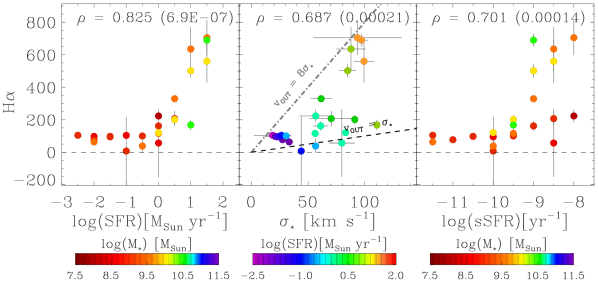
Figure 20: Outflow velocity as given by $(v_{\rm 0.1\leavevmode\nobreak\ gas}^{2}-v_{\rm 99.9\leavevmode\nobreak\ stars}^{2})^{1/2}$ (see explanation in $\S$ 4.1) inferred from [OIII] (upper panel) and H$\alpha$ emission (bottom panel), plotted as a function of SFR, stellar velocity dispersion (as obtained from the fit to the stellar continuum), and sSFR. The same bins as Fig. 17 are plotted, excluding those for which $(v_{\rm 0.1\leavevmode\nobreak\ gas}^{2}-v_{\rm 99.9\leavevmode\nobreak\ stars}^{2})<0$. In the middle panels, the black dashed lines indicate the locus where $v_{\rm out}=\sigma_{\rm stars}$, and the grey dot-dashed lines indicate the approximate upper envelopes of the distributions of values, given by the relationships: $v_{\rm out}=6\sigma_{\rm stars}$ for [OIII], and $v_{\rm out}=6\sigma_{\rm stars}$ for H$\alpha$. The Spearman rank correlation coefficient ($0<\rho<1$, higher values of $\rho$ indicate stronger correlation) is reported for each plot, along with the corresponding two-sided p-value (if the p-value is $\leq\alpha$, where $\alpha=0.05$ is the level of significance, the observed correlation is statistically significant).

Figures 19 and 20 show the outflow velocity ($v_{\rm out}$) as a function of galaxy properties (e.g. SFR, $\sigma_{*}$ and sSFR), for two different estimates of the outflow velocity, indicated as $v_{\rm out,low}$ and $v_{\rm out,high}$, probing respectively the low and the high velocity gas within the ionised outflows, and defined as $v_{\rm out,low}\equiv(v_{\rm 15.9\leavevmode\nobreak\ gas}^{2}-v_{\rm 84.1\leavevmode\nobreak\ stars}^{2})^{1/2}$ and $v_{\rm out,high}\equiv(v_{\rm 0.1\leavevmode\nobreak\ gas}^{2}-v_{\rm 99.9\leavevmode\nobreak\ stars}^{2})^{1/2}$. We note that in the middle panels of Fig. 19 and 20 the outflow velocity is shown as a function of the stellar velocity dispersion instead of the stellar mass, so that these trends can be readily compared to the predictions of models of star formation-driven feedback. Figures 19 and 20 indicate that the outflow velocity scales with SFR and sSFR. In particular, $v_{\rm out,high}$, shows a very tight ($\rho>0.8$) correlation with the SFR. Previous studies found a similar increase of outflow speed with SFR (e.g. Martin 2005 using a sample of IR luminous galaxies at $z\sim 0$; Arribas et al. 2014 for outflows detected in $z\sim 0$ (U)LIRGs; Chisholm et al. 2014 in local star forming and starburst galaxies; Heckman et al. 2011 and Heckman et al. 2015 using a a sample of UV-luminous starbursts and Lyman break analogs at $z\sim 0$, Bradshaw et al. 2013 and Weiner et al. 2009 by means of a stacking analysis of star forming galaxies at the typical redshifts of $z\sim 1.2$ and $z\sim 1.4$, respectively) and with sSFR (Bradshaw et al., 2013; Heckman et al., 2015). However, the correlations found by previous studies are in most cases less significant than in our study, and inevitably based on smaller number statistics. Furthermore, the literature also reports many cases in which observations failed at finding a clear correlation between outflow velocity and SFR (e.g. Heckman et al. 2000, Rupke et al. 2005, Chen et al. 2010, and Westmoquette et al. 2012 at $z\sim 0$ ; Sato et al. 2009 at $z\sim 0.4$; Rubin et al. 2014 at $z\sim 0.5$; Kornei et al. 2012 and Martin et al. 2012 at $z\sim 1$; Erb et al. 2012 at $z\sim 1.5$). In most cases, the main issue appears to be the narrow dynamical range of host galaxy properties probed by such outflow studies, which is crucial to recover scaling relations (Rupke et al., 2005; Westmoquette et al., 2012; Martin et al., 2012). Inspection of Figs. 19 and 20 suggests that a strong correlation between outflow velocity and SFR is characteristic of galaxies with $\rm log(SFR[M_{\odot}\leavevmode\nobreak\ yr^{-1}])\gtrsim 0$; at $\rm log(SFR[M_{\odot}\leavevmode\nobreak\ yr^{-1}])<0$ the dependence of $v_{\rm out}$ on SFR is nearly flat.

Overall we find that the outflow velocity increases with the stellar velocity dispersion, as shown by Fig. 20 (a positive correlation between $v_{\rm out,high}$ and $\sigma_{*}$ is observed with $\rho>0.6$ and p-value$\ll 0.05$ for both [OIII] and H$\alpha$ outflows) and, to some extent, also by Fig. 19 (a weak correlation between $v_{\rm out,low}$ and $\sigma_{*}$ is found for [OIII], although not for H$\alpha$). While the existence of a correlation between gas velocity and SFR is a more or less established property of galactic outflows, the relationship with stellar mass (or with the dynamical mass, as probed by the galaxy rotation speed or by the stellar velocity dispersion) is more controversial. Lehnert & Heckman (1996), in their sample of local, edge-on IR luminous galaxies did not find any relationship between the kinematical properties (emission line widths, velocity shear) of the ionised gas, as measured along the minor axis of the disks (where outflows are found to dominate the gas kinematics), and galaxy rotation speeds. Similarly, Heckman et al. (2000) showed that the NaI outflow velocity is unrelated to the galaxy rotational velocity. On the contrary, Martin (2005) found an almost linear relation with galaxy rotation speed (although they could only test this relationship for a small fraction of the galaxy sample with available rotation curves). The positive correlation between maximum outflow velocity and galaxy circular velocity found by Rupke et al. (2005) is completely driven by the dwarf starburst sample of Schwartz & Martin (2004), highlighting once again the importance of probing a wide dynamical range in galaxy properties. In line with this hypothesis, Arribas et al. (2014) found that the distribution of ionised outflow velocity as a function of galaxy dynamical mass is rather scattered in the (U)LIRG regime, i.e. for massive and highly star forming galaxies. The results by Heckman et al. (2011), whose sample spans a wider range of galaxy properties, suggest that outflow velocity and stellar mass are instead related. Studies at higher redshifts seem to find more consistently a correlation between outflow velocity and M_∗ in star forming galaxies (Weiner et al., 2009; Bradshaw et al., 2013; Rubin et al., 2014).

Higher stellar velocity dispersions trace deeper gravitational potentials. The positive correlation that we observe in Fig. 20 between $v_{\rm out,high}$ and $\sigma_{*}$ suggests that ionised outflows may still gain a velocity sufficiently high for gas to escape also from massive galaxies, and not only from lower-mass galaxies (as it would be the case if the outflow velocity did not depend on M_∗, in which case the escape of the gas from low-mass galaxies would be favoured). However, we note that our analysis may be biased towards higher velocity outflows. Indeed, our method probably selects only outflows with velocity close to or above the escape velocity from the galaxy, because we are selecting gas velocities in excess of the stellar velocity in order to avoid contamination by gas in virial motion. Figure 20 also shows that, for a fixed SFR, the outflow velocity (in the high velocity regime) decreases with $\sigma_{*}$. A possible explanation is that for a given SFR, i.e. for a given energy and momentum budget available to accelerate the gas, outflows are slowed down and re-captured by the gravitational potential in more massive galaxies, and therefore they become increasingly ineffective at higher masses.

The relationships between outflow velocity and stellar velocity dispersion (central panels of Figs. 19 and 20) suggest that the physical mechanisms powering the lower and the higher velocity clouds in the observed ionised outflows may be slightly different. Indeed, at lower velocities ($v_{\rm out,low}$), which trace the bulk of the gas in outflow , the data points are placed just below the $v_{\rm out}=\sigma_{*}$ locus, indicating that radiation pressure-driven (or “momentum-driven”) winds, which are characterised by $v_{\rm out}\gtrsim 2\sigma_{*}$ (Murray et al., 2005; Davé et al., 2011b), are unlikely to dominate in this regime. Instead, these outflows may be generated by the kinetic energy injected into the ISM by supernovae and stellar winds, i.e. “energy-driven”. Similarly, Bouché et al. (2012), by using background quasars to trace MgII blueshifted absorption in $z\sim 0$ galaxies, estimated outflow speeds that are on average half the escape velocity, although these authors did not find any correlation with the SFR. On the other hand, the situation changes significantly in the high velocity regime, as shown by Fig. 20, where the data lie mostly above the $v_{\rm out}=\sigma_{*}$ relationship. In this case, momentum-driven winds may also be at play (see also findings by Martin 2005, Heckman et al. 2015 for what they define as “strong outflows” at $z\sim 0$, and by Weiner et al. 2009, at $z\sim 1.4$). Figure  20 also suggests that the asymptotic velocity of the observed ionised outflows is as high as $6-8\leavevmode\nobreak\ \sigma_{\rm stars}$, i.e. comparable to or higher than the escape velocity ($v_{\rm esc}\simeq(5-6)\sigma_{*}$, where $\sigma_{*}$ is the line-of-sight stellar velocity dispersion, gives a conservative estimate of the escape velocity, e.g. Weiner et al. 2009).

4.2 The connection between galactic outflows and the main sequence of star-forming galaxies

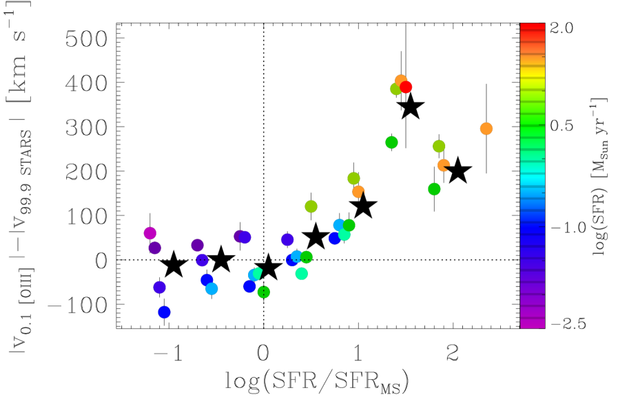
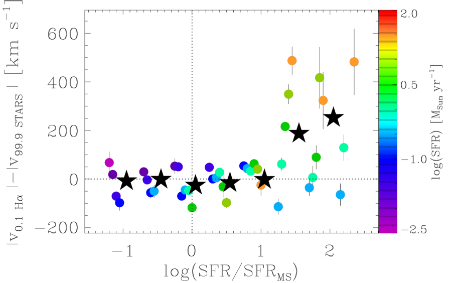
Figure 21: Excess of line-of-sight velocity of the ionised gas with respect to the stars (${v_{\rm gas}-v_{\rm stars}}$) as given by ${y=|v_{\rm 0.1\leavevmode\nobreak\ gas}|-|v_{\rm 99.9\leavevmode\nobreak\ stars}|}$, plotted as a function of the offset from the local MS of star-forming galaxies. In the upper panel the outflow velocity is measured from [OIII] and in the lower panel from H$\alpha$. As in Fig. 17, only bins with either $\sigma_{y}<{\rm 50\leavevmode\nobreak\ km\leavevmode\nobreak\ s^{-1}}$ or ${|y|\geq 2\sigma_{y}}$ are shown. The black stars indicate the mean trend, obtained by averaging the data points (weighted with their errors) over bins of ${\rm\Delta log(SFR/SFR_{MS})=0.5}.$

Galactic outflows and cosmic inflows are invoked as key moderators of the SFR (and sSFR) in galaxies through cosmic times. Specifically, powerful galactic-scale outflows driven by AGNs and/or by extreme starburst episodes (possibly merger-driven) are thought to constitute the observational evidence for the so called “quenching” mechanism acting on galaxies at all cosmic times (or “mass-quenching”, distinct from the “environment-quenching”, Peng et al. 2010, 2012). Such mechanism, through different physical processes yet poorly understood, should eventually transforms disky star-forming galaxies into passive spheroids, thus generating the observed dichotomy between blue star forming and red passive galaxies (Baldry et al., 2004). Cosmic inflows are believed to feed galaxies through a smooth and continuous process, hence directly regulating the rate at which star formation occurs (Dekel et al., 2009; Bouché et al., 2010; Lilly et al., 2013). The tight correlation between stellar mass and SFR observed from $z\sim 0$ up to $z\sim 4$ (Schreiber et al., 2015) provides the major observational support to the hypothesis of a “cosmic feeding of star formation”, but direct observational evidence is still lacking.

In this scenario there is an effect that has been little explored from an observational point of view, that is the possible role of galactic outflows in shaping the MS of star forming galaxies and, in particular, its upper envelope. Figure 18 shows that ionised outflows are detected only in galaxies located above the MS on the ${\rm M_{*}-SFR}$ diagram. This effect can be visualised even better in Fig. 21, where we plotted the excess of line-of-sight velocity of the ionised gas with respect to the stars, i.e. ${|v_{\rm 0.1\leavevmode\nobreak\ gas}|-|v_{\rm 99.9\leavevmode\nobreak\ stars}|}$ (for both [OIII] and H$\alpha$), as a function of the offset from the local MS (as derived in $\S$ 2.2). Figure 21 shows a sharp increase of outflows at $\rm SFR>SFR_{MS}$, where, for a given stellar mass, $\rm SFR_{MS}$ represents the SFR of a galaxy located on the MS. In other words, we empirically observe that for a given stellar mass, when the SFR exceeds SFR_MS, the gas velocity increases significantly, with the effect of producing observable outflows. These outflows may eventually contribute to the suppression of the SFR by reducing gas available for star formation, therefore bringing the galaxy back onto the MS. Our observational result may reveal a self-adjusting mechanism that explains the tightness of the local MS (i.e. $\pm 0.3$ dex). We note that this hypothesis is consistent with the scenario recently proposed by Tacchella et al. (2015), who used simulations of high-redshift star forming galaxies to explore the mechanisms that confine galaxies into a narrow sequence in the ${\rm M_{*}-SFR}$ plane.

The picture emerging from Figs. 18 and 21 is consistent with the abundant observational evidence for outflows in local starbursts and (U)LIRGs. Outflows of ionised, neutral and molecular gas are a common feature of galaxies with intense star formation activity, as traced by their high infrared luminosities $L_{\rm IR}(8-1000\leavevmode\nobreak\ {\rm\mu m})\geq 10^{11}L_{\odot}$ (Chung et al., 2011; Sturm et al., 2011; Westmoquette et al., 2012; Rupke & Veilleux, 2013; Rodríguez Zaurín et al., 2013; Veilleux et al., 2013; Spoon et al., 2013; Bellocchi et al., 2013; Cazzoli et al., 2014; Arribas et al., 2014; Cicone et al., 2014). These galaxies have larger SFR and sSFR than local MS galaxies (i.e. ${\rm SFR>10\leavevmode\nobreak\ M_{\odot}yr^{-1}}$ and sSFR typically higher than ${\rm 10^{-9}yr^{-1}}$, e.g. Combes et al. 2013) and populate the upper-right region of the M_∗–SFR diagram. Previous observations at $z\sim 0$ are therefore consistent with our findings, i.e. that star formation-driven galactic outflows are preferentially hosted by galaxies located above the local MS in the ${\rm M_{*}-SFR}$ diagram.

On the contrary, except from Martin et al. (2012), outflows searches at higher redshifts revealed in general no dependency of galactic outflows on the galaxy position on the ${\rm M_{*}-SFR}$ diagram with respect to the MS (Rubin et al., 2014; Genzel et al., 2014; Förster Schreiber et al., 2014), although in some of these cases the observed outflows are plausibly driven by AGNs (Genzel et al., 2014; Förster Schreiber et al., 2014). The majority of NaID outflows detected by Sato et al. (2009) are hosted by galaxies lying on the red sequence in the rest-frame $(U-B)$ color vs $M_{B}$ diagram and showing early-type morphologies. These authors however note that most of the red sequence galaxies with detectable outflows in their sample may have some residual star formation, as suggested by their still high IR luminosities, and/or show signs of recent star formation, as indicated by their $NUV-R_{AB}$ color. Furthermore, since AGNs are not excluded from their sample, an accreting super massive black hole may be responsible for driving the observed outflows, especially in those galaxies which do not show significant star formation activity.

We note that there are secondary effects emerging from Fig. 21. On the one hand, outflows seem to “saturate” at $\rm log(SFR/SFR_{MS})>1.5$ when using [OIII] as a tracer, while the scatter on the corresponding plot derived using H$\alpha$ does not allow us to assess whether a similar saturation is present also for this tracer or not. On the other hand, the minimum ${\rm SFR/SFR_{MS}}$ required to launch observable outflows seems to be lower (i.e. closer to 1) for [OIII], while it is about a factor of 10 larger for H$\alpha$.

An indirect implication of Fig. 21 is that galaxies located on or just below the local MS do not host significant outflows, although we cannot exclude the presence of low-velocity outflows (“weak outflows”, e.g. Heckman et al. 2015), or of fewer galaxies with important outflow activity but where the outflow is seen edge-on. This implies that star formation-driven outflows are likely not responsible for the migration of blue star forming galaxies into the “red sequence”, and so they are not responsible for what we generally refer to as “quenching”, consistent with what is found by simulations (Hopkins et al., 2012) and also consistent with recent observational evidence that, for most galaxies, quenching results from the cutoff of gas inflow (a process refereed to as “strangulation” or “starvation”, Peng et al. 2015). However, our results clearly highlight a link between high sSFRs (i.e. sSFR in excess with respect to MS galaxies) and fast star formation-driven outflows.

5 Summary and conclusions

Galactic outflows, ejecting gas out of the galaxy, are a manifestation of feedback. Powerful outflows have been observed in galaxies for decades, however it is still not clear what is their role in galaxy evolution and whether they are actually responsible for reducing or, in the most extreme cases, shutting off star formation in galaxies. Some key questions that we have addressed in this work are: how can we reliably trace galactic outflows and estimate their properties? How do outflow properties relate to the properties of the host galaxy? How do outflow properties compare to the predictions of galaxy evolutionary models?

The most obvious source of feedback in galaxies is star formation itself, which, by conveying energy and momentum to the interstellar medium over prolonged timescales, can potentially affect future star formation and hence galaxy evolution. In this paper we have investigated the presence and properties of star formation-driven outflows of ionised gas in normal galaxies by using a large spectroscopic sample of $\sim 160,000$ local non-active galaxies drawn from the SDSS. The galaxy sample was divided into a fine grid of bins in the $\rm M_{*}-SFR$ parameter space, for each of which we produced a composite spectrum by stacking together the SDSS spectra of the galaxies contained in that bin. We exploited the high signal-to-noise of the stacked spectra to study the emergence of faint features of optical emission lines that trace galactic outflows, which otherwise would be too faint to detect in individual galaxy spectra. Not only has the stacking technique allowed us to explore the presence of galactic outflows in a large and representative sample of normal galaxies, spanning a wide range of galaxy properties (${\rm M_{*}\in[2\times 10^{7},6\times 10^{11}]\leavevmode\nobreak\ M_{\odot}}$ and ${\rm SFR\in[2\times 10^{-3},2\times 10^{2}]\leavevmode\nobreak\ M_{\odot}\leavevmode\nobreak\ yr^{-1}}$), but also to break the degeneracy between SFR and M_∗ that affects the bulk of the local star forming galaxy population (i.e. the MS galaxies).

Based on the assumption that feedback-related processes (outflows, turbulence) should affect only the gas kinematics, leaving the motions of stellar populations unperturbed, we traced the kinematical signature of feedback by adopting a novel approach that relies on the comparison between the LoSVD of the ionised gas (as traced by the [OIII] and H$\alpha$+[NII] emission lines) and the LoSVD of the stars, which were used as a reference tracing virial motions. More specifically, significant deviations of the ionised gas kinematics from the stellar kinematics in the high velocity tails of the LoSVDs (to minimise the effects of virial motions and turbulence) were interpreted as a signature of outflows.

Our results suggest that the incidence of ionised outflows in local star forming galaxies increases with SFR and sSFR. Moreover, at a given SFR, more massive galaxies are increasingly less efficient at launching powerful outflows. In galaxy stacks displaying the clearest signature of galactic outflows, the outflow velocity ($v_{\rm out}$) was found to correlate tightly with the SFR for ${\rm SFR>1\leavevmode\nobreak\ M_{\odot}\leavevmode\nobreak\ yr^{-1}}$, whereas at lower SFRs the dependance of $v_{\rm out}$ on SFR appears nearly flat. The outflow velocity, although with a much larger scatter, increases also with the stellar velocity dispersion ($\sigma_{*}$), and in a few galaxy stacks reaches values as high as $v_{\rm out}\sim(6-8)\sigma_{*}$, indicating that both energy-driven and momentum-driven winds may be at play.

Strikingly, the kinematical signature of ionised outflows was detected only in galaxies located above the main sequence of star forming galaxies in the ${\rm M_{*}-SFR}$ diagram, and the incidence of high velocity outflows increases sharply with the offset from the MS. On the one hand, this result clearly highlights a link between (specific) star formation rates in excess with respect to MS galaxies and fast star formation-driven outflows, suggesting that such outflows may be responsible for shaping the upper envelope of the MS by providing a self-regulating mechanism for star formation. On the other hand, our findings suggest that the observed outflows may have little or no role in the “quenching” of star formation in galaxies, i.e. the migration of blue star forming galaxies into the “red sequence”.

Finally, although our study focussed mainly on galactic outflows, a complementary analysis of the stellar kinematics revealed blue asymmetries (of a few 10 km s^-1) in the stellar LoSVDs of galaxies with higher SFRs and M_∗. The large uncertainties did not allow us to draw any firm conclusion about the origin of such asymmetries, but a possibility is that these trace the presence of a large number of runaway stars and hypervelocity stars in radial trajectories within local galaxies.

In this paper, besides demonstrating the advantages and limitations of applying the spectral stacking technique to optical emission lines for outflow studies, we proposed a new strategy to study galactic outflows, which relies on the direct comparison between the LoSVD of the gas and the LoSVD of the stars. Such a new approach was tested with the SDSS spectroscopic sample that, although certainly valuable for its large statistics, is obviously limited in terms of spatial information. However, this methodology can reveal its full potential if applied to resolved (IFS) observations of large galaxy samples, which are becoming available thanks to the ongoing IFS surveys (MaNGA, CALIFA and SAMI) and new powerful instruments such as MUSE.

Appendix A The percentile velocities of the LoSVDs

Figures 22, 23, 24, 25 and 26 show, respectively, the 15.9th (-$\sigma$), 2.3th (-2$\sigma$), 84.1th ($\sigma$), 97.7th (2$\sigma$) and 99.9th (3$\sigma$) percentile velocities of the [OIII], H$\alpha$ and stellar LoSVDs as a function of SFR, M_∗ and sSFR. The results of the Spearman rank test performed on these relationships are reported in Table 1. See further discussion in $\S$ 3.2.

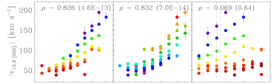
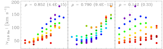
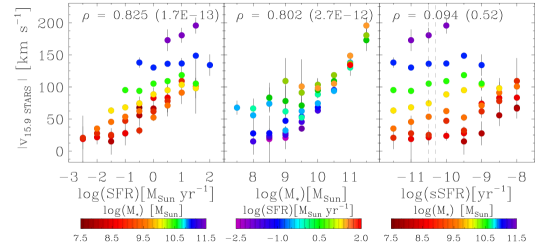
Figure 22: (Modulus of the) 15.9th percentile velocity of LoSVD of the ionised gas as traced by the [OIII] (top panel) and H$\alpha$ (middle panel) emission lines, and of the stars (bottom panel). For a Gaussian velocity distribution, the 15.9th percentile velocity corresponds to -1 standard deviation ($-\sigma$) from the mean velocity. Similarly to Fig. 14, we report for each plot the Spearman rank correlation coefficient $\rho$ along with its associated two-sided p-value.

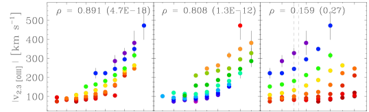
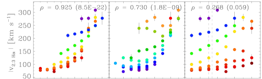
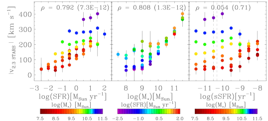
Figure 23: (Modulus of the) 2.3th percentile velocity of the LoSVD of the ionised gas as traced by the [OIII] (top panel) and H$\alpha$ (middle panel) emission lines, and of the stars (bottom panel). For a Gaussian velocity distribution, the 2.3th percentile velocity corresponds to -2 standard deviations ($-2\sigma$) from the mean velocity. Similarly to Fig. 14, we report for each plot the Spearman rank correlation coefficient $\rho$ along with its associated two-sided p-value.

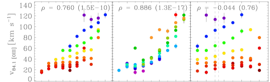
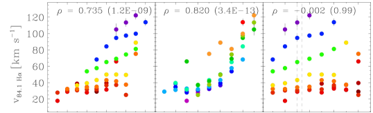
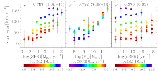
Figure 24: 84.1th percentile velocity of the LoSVD of the ionised gas as traced by the [OIII] (top panel) and H$\alpha$ (middle panel) emission lines, and of the stars (bottom panel). For a Gaussian velocity distribution, the 84.1th percentile velocity corresponds to +1 standard deviation ($\sigma$) from the mean velocity. Similarly to Fig. 14, we report for each plot the Spearman rank correlation coefficient $\rho$ along with its associated two-sided p-value.

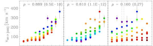
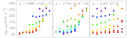
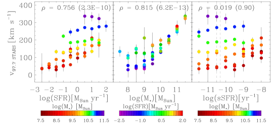
Figure 25: 97.7th percentile velocity of the LoSVD of the ionised gas as traced by the [OIII] (top panel) and H$\alpha$ (middle panel) emission lines, and of the stars (bottom panel). For a Gaussian velocity distribution, the 97.7th percentile velocity corresponds to +2 standard deviations ($2\sigma$) from the mean velocity. Similarly to Fig. 14, we report for each plot the Spearman rank correlation coefficient $\rho$ along with its associated two-sided p-value.

Figure 26: 99.9th percentile velocity of the LoSVD of the ionised gas as traced by the [OIII] (top panel) and H$\alpha$ (middle panel) emission lines, and of the stars (bottom panel). For a Gaussian velocity distribution, the 99.9th percentile velocity corresponds to +3 standard deviations ($3\sigma$) from the mean velocity. Similarly to Fig. 14, we report for each plot the Spearman rank correlation coefficient $\rho$ along with its associated two-sided p-value.