Scalable Constrained Clustering:
A Generalized Spectral Method

Abstract

We present a simple spectral approach to the well-studied constrained clustering problem. It captures constrained clustering as a generalized eigenvalue problem with graph Laplacians. The algorithm works in nearly-linear time and provides concrete guarantees for the quality of the clusters, at least for the case of 2-way partitioning. In practice this translates to a very fast implementation that consistently outperforms existing spectral approaches both in speed and quality.

1 Introduction

Clustering with constraints is a problem of central importance in machine learning and data mining. It captures the case when information about an application task comes in the form of both data and domain knowledge. We study the standard problem where domain knowledge is specified as a set of soft must-link (ML) and cannot-link (CL) constraints [1].

The extensive literature reports a plethora of methods, including spectral algorithms that explore various modifications and extensions of the basic spectral algorithm by Shi and Malik [18] and its variant by Ng et al. [15].

The distinctive feature of our algorithm is that it constitutes a natural generalization, rather than an extension of the basic spectral method. The generalization is based on a critical look at how existing methods handle constraints, in section 3. The solution is derived from a geometric embedding obtained via a spectral relaxation of an optimization problem, exactly in the spirit of [15, 18]. This is depicted in the workflow in Figure 1. Data and ML constraints are represented by a Laplacian matrix $L$ and CL constraints by another Laplacian matrix $H$. The embedding is realized by computing a few eigenvectors of the generalized eigenvalue problem $Lx=\lambda Hx$. The generalization of [15, 18] lies essentially in $H$ being a Laplacian matrix rather than the diagonal $D$ of $L$. In fact, as we will discuss later, $D$ itself is equivalent to a specific Laplacian matrix; thus our method encompasses the basic spectral method as a special case of constrained clustering.

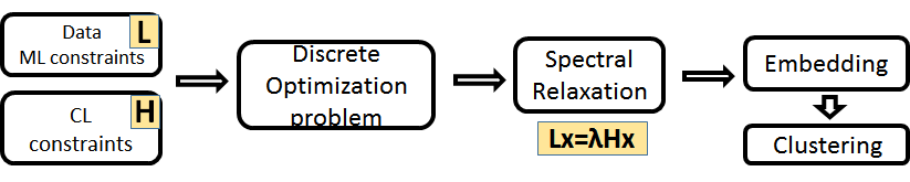
Figure 1: A schematic overview of our approach.

Our approach is characterized by its conceptual simplicity that enables a straightforward mathematical derivation of the algorithm, possibly the simplest among all competing spectral methods. Reducing the problem to a relatively simple generalized eigensystem enables us to derive directly from recent significant progress due to Lee et al. [12] in the theoretical understanding of the standard spectral clustering method, offering its first practical realization. In addition, the algorithm comes with two features that are not simultaneously shared by any of the prior methods: (i) it is provably fast by design as it leverages fast linear system solvers for Laplacian systems [9] (ii) it provides a concrete theoretical guarantee for the quality of 2-way constrained partitioning, with respect to the underlying discrete optimization problem, via a generalized Cheeger inequality (section 6).

In practice, our method is at least 10x faster than competing methods on large data sets. It solves data sets with millions of points in less than 2 minutes, on very modest hardware. Furthermore the quality of the computed segmentations is often dramatically better.

2 Problem definition

The constrained clustering problem is specified by three weighted graphs:

1. The data graph $G_{D}$ which contains a given number of $k$ clusters that we seek to find. Formally, the graph is a triple $G_{D}=(V,E_{D},w_{D})$, with the edge weights $w_{D}$ being positive real numbers indicating the level of `affinity' of their endpoints.

2. The knowledge graphs $G_{ML}$ and $G_{CL}$. The two graphs are formally triples $G_{ML}=(V,E_{ML},w_{ML})$ and $G_{CL}=(V,E_{CL},w_{CL})$. Each edge in $G_{ML}$ indicates that its two endpoints should be in the same cluster, and each edge in $G_{CL}$ indicates that its two endpoints should be in different clusters. The weight of an edge indicates the level of belief placed in the corresponding constraint.

We emphasize that prior knowledge does not have to be exact or even self-consistent, and thus the constraints should not be viewed as `hard' ones. However, to conform with prior literature, we will use the existing terminology of `must link' (ML) and `cannot link' (CL) constraints to which $G_{ML}$ and $G_{CL}$ owe their notation respectively.

In the constrained clustering problem the general goal is to find $k$ disjoint clusters in the data graph. Intuitively, the clusters should result from cutting a small number of edges in the data graph, while simultaneously respecting as much as possible the constraints in the knowledge graphs.

3 Re-thinking constraints

Many approaches have been pursued within the constrained spectral clustering framework. They are quite distinct but do share a common point of view: constraints are viewed as entities structurally extraneous to the basic spectral formulation, necessitating its modification or extension with additional mathematical features. However, a key fact is overlooked:

Standard clustering is a special case of constrained clustering with implicit soft ML and CL constraints.

To see why, let us briefly recall the optimization problem in the standard method (Ncut).

$$\phi=\min_{S\subseteq V}\frac{cut_{G_{D}}(S,\bar{S})}{vol(S)vol(\bar{S})/vol(V)}.$$

Here $vol(S)$ denotes the total weight incident to the vertex set $S$, and $cut_{G}(S,\bar{S})$ denotes the total weight crossing from $S$ to $\bar{S}$ in $G$.

The data graph $G_{D}$ is actually an implicit encoding of soft ML constraints. Indeed, pairwise affinities between nodes can be viewed as `soft declarations' that such nodes should be connected rather than disconnected in a clustering. Let now $d_{i}$ denote the total incident weight of vertex $i$ in $G_{D}$. Consider the demand graph $K$ of implicit soft CL constraints, defined by the adjacency $K_{ij}=d_{i}d_{j}/vol(V)$. It is easy to verify that $vol(S)vol(\bar{S})/vol(V)=cut_{K}(S,\bar{S})$. We have

$$\min_{S\subseteq V}\frac{cut_{G_{D}}(S,\bar{S})}{vol(S)vol(\bar{S})/vol(V)}=\min_{S\subseteq V}\frac{cut_{G_{D}}(S,\bar{S})}{cut_{K}(S,\bar{S})}.$$

In other words, the Ncut objective can be viewed as:

$$\min_{S\subseteq V}\frac{\textnormal{weight of cut (violated) implicit ML constraints}}{\textnormal{weight of cut (satisfied) implicit CL constraints}}.$$ (1)

With this realization, it becomes evident that incorporating the knowledge graphs ($G_{ML},G_{CL}$) is mainly a degree-of-belief issue, between implicit and explicit constraints. Yet all existing methods insist on handling the explicit constraints separately. For example, [17] modify the Ncut optimization function by adding in the numerator the number of violated explicit constraints (independently of them being ML or CL), times a parameter $\gamma$. In another example, [25] solve the spectral relaxation of Ncut, but under the constraint that the number of satisfied ML constraints minus the number of violated CL constraints is lower bounded by a parameter $\alpha$. Despite the separate handling of the explicit constraints, degree-of-belief decisions (reflected by parameters $\alpha$ and $\gamma$) are not avoided. The actual handling also appears to be somewhat arbitrary. For instance, most methods take the constraints unweighted, as usually provided by a user, and handle them uniformly; but it is unclear why one constraint in a densely connected part of the graph should be treated equally to another constraint in a less well-connected part. Moreover, most prior methods enforce the use of the balance implicit constraints in $K$, without questioning their role, which may be actually adverserial in some cases. In general, the mechanisms for including the explicit constraints are oblivious of the input, or even of the underlying algebra.

Our approach. We choose to temporarily drop the distinction of the constraints into explicit and implicit. We instead assume that we are given one set of ML constraints, and one set of CL constraints, in the form of weighted graphs $G$ and $H$. We then design a generalized spectral clustering method that retains the $k$-way version of the objective shown in equation 1. We apply this generalized method to our original problem, after a merging step of the explicit and implicit CL/ML constraints into one set of CL/ML constraints.

The merging step can be left entirely up to the user, who may be able to exploit problem-specific information and provide their choice of weights for $G$ and $H$. Of course, we expect that in most cases explicit CL and ML constraints will be provided in the form of simple unweighted graphs $G_{ML}$ and $G_{CL}$. For this case we provide a simple method that resolves the degree-of-belief issue and constructs $G$ and $H$ automatically. The method is heuristic, but not oblivious to the data graph, as they adjust to it.

4 Related Work

The literature on constrained clustering is quite extensive, as the problem has been pursued under various guises from different communities. Here we present a short and unavoidably partial review.

A number of methods incorporate the constraints via only modifying the data matrix in the standard method. In certain cases some or all of the CL constraints are dropped in order to prevent the matrix from turning negative [5, 14]. The formulation of [17] incorporates all constraints into the data matrix, essentially by adding a signed Laplacian, which is a generalization of the Laplacian for graphs with negative weights; notably, their algorithm does not solve a spectral relaxation of the problem but attempts to solve the (hard) optimization problem exactly, via a continuous optimization approach.

A different approach is proposed in [13]: constraints are used in order to improve the embedding obtained through the standard problem, before applying the partitioning step. In principle this embedding-processing step is orthogonal to methods that compute some embedding (including ours), and it can be used to potentially improve them.

A number of other works use the ML and CL constraints to super-impose algebraic constraints onto the spectral relaxation of the standard problem. These additional algebraic constraints usually yield much harder constrained optimization problems [3, 6, 26, 25].

Besides our work, there exists a number of other approaches that reduce constrained clustering into generalized eigenvalue problems $Ax=\lambda Bx$ that deviate substantially from than the standard formulation. These methods can be implemented to run fast, as long as: (i) linear systems in $A$ can be solved efficiently, (ii) $A$ and $B$ are positive semi-definite. Specifically, [27, 28] use a generalized eigenvalue problem in which $B$ is a diagonal, but $A$ is not generally amenable to existing efficient linear system solvers. In [25] matrix $A$ is set to be the normalized Laplacian of the data graph (implicitly attempting to impose the standard balance constraints), and $B$ has both positive and negative off-diagonal entries representing ML and CL constraints respectively. In the general case $B$ is not positive, forcing the computation of full eigenvalue decompositions. However the method can be modified to use a (positive) signed Laplacian as the matrix $B$, as partially observed in [24]. This modification has a fast implementation. The formulation in [17] also leads to a fast implementation of its spectral relaxation.

5 Algorithm and its derivation

5.1 Graph Laplacians

Let $G=(V,E,w)$ be a graph with positive weights. The Laplacian $L_{G}$ of $G$ is defined by $L_{G}(i,j)=-w_{ij}$ and $L_{G}(i,i)=\sum_{j\neq i}w_{ij}$. The graph Laplacian satisfies the following basic identity for all vectors $x$:

$$x^{T}L_{G}x = \sum_{i,j}w_{ij}(x_{i}-x_{j})^{2}.$$ (2)

Given a cluster $C\subseteq V$ we define a cluster indicator vector by $x_{C}(i)=1$ if $i\in C$ and $x_{C}(i)=0$ otherwise. We have:

$$x_{C}^{T}L_{G}x_{C}=cut_{G}(C,\bar{C})$$ (3)

where $cut_{G}(C,\bar{C})$ denotes the total weight crossing from $C$ to $\bar{C}$ in $G$.

5.2 The optimization problem

As we discussed in section 3, we assume that the input consists of two weighted graphs, the must-link constraints $G$, and the cannot-link constraints $H$.

Our objective is to partition the node set $V$ into k disjoint clusters $C_{i}$. We define an individual measure of badness for each cluster $C_{i}$:

$$\phi_{i}(G,H)=\frac{cut_{G}(C_{i},\bar{C_{i}})}{cut_{H}(C_{i},\bar{C_{i}})}$$ (4)

The numerator is equal to the total weight of the violated ML constraints, because cutting one such constraint violates it. The denominator is equal to the total weight of the satisfied CL constraints, because cutting one such constraint satisfies it. Thus the minimization of the individual badness is a sensible objective.

We would like then to find clusters $C_{1},\ldots,C_{k}$ that minimize the maximum badness, i.e. solve the following problem:

$${\Phi}_{k}=\textnormal{{\bf min} $\max_{i}{\phi_{i}}$}.$$ (5)

Using equation 3, the above can be captured in terms of Laplacians: letting $x_{C_{i}}$ denote the indicator vector for cluster $i$, we have

$${\phi}_{i}(G,H)=\frac{x_{C_{i}}^{T}L_{G}x_{C_{i}}}{x_{C_{i}}^{T}L_{H}x_{C_{i}}}.$$

Therefore, solving the minimization problem posed in equation 5 amounts to finding $k$ vectors in $\{0,1\}^{n}$ with disjoint support.

Notice that the optimization problem may not be well-defined in the event that there are very few CL constraints in $H$. This can be detected easily and the user can be notified. The merging phase also takes automatically care of this case. Thus we assume that the problem is well-defined.

5.3 Spectral Relaxation

To relax the problem we instead look for $k$ vectors in $y_{1},\ldots,y_{k}\in{\mathbb{R}}^{n}$, such that for all $i\neq j$, we have $y_{i}L_{H}y_{j}=0$. These $L_{H}$-orthogonality constraints can be viewed as a relaxation of the disjointness requirement. Of course their particular form is motivated by the fact that they directly give rise to a generalized eigenvalue problem. Concretely, the $k$ vectors $y_{i}$ that minimize the maximum among the $k$ Rayleigh quotients $(y_{i}^{T}L_{G}y_{i})/(y_{i}^{T}L_{H}y_{i})$ are precisely the generalized eigenvectors corresponding to the $k$ smallest eigenvalues of the problem: $L_{G}x=\lambda L_{H}x.$ This fact is well understood and follows from a generalization of the min-max characterization of the eigenvalues for symmetric matrices; details can be found for instance in [19].

Notice that $H$ does not have to be connected. Since we are looking for a minimum, the optimization function avoids vectors that are in the null space of $L_{H}$. That means that no restriction needs to be placed on $x$ so that the eigenvalue problem is well defined, other than it can't be the constant vector (which is in the null space of both $L_{G}$ and $L_{H}$), assuming without loss of generality that $G$ is connected.

5.4 The embedding

Let $X$ be the $n\times k$ matrix of the first $k$ generalized eigenvectors for $L_{G}x=\lambda L_{H}x$. The embedding is shown in Figure 2.

We discuss the intuition behind the embedding. Without step 4 and with $L_{H}$ replaced with the diagonal $D$, the embedding is exactly the one recently proposed and analyzed in [12]. It is a combination of the embeddings considered in [18, 15, 23], but the first known to produce clusters with approximation guarantees. The generalized eigenvalue problem $Lx=\lambda Dx$ can be viewed as a simple eigenvalue problem over a space endowed with the $D$-inner product: $\left<x,y\right>_{D}=x^{T}Dy$. Step 5 normalizes the eigenvectors to a unit $D$-norm, i.e. $x^{T}Dx=1$. Given this normalization, it is shown in [12] that the rows of $U$ at step 7 (vectors in $k$-dimensional space) are expected to concentrate in $k$ different directions. This justifies steps 8-10 that normalize these row vectors onto the $k$-dimensional sphere, in order to concentrate them in a spatial sense. Then a geometric partitioning algorithm can be applied.

0:  $X,L_{H},d$

0:  embedding $U\in{\mathbb{R}}^{n\times k}$, $l\in{\mathbb{R}}^{n\times 1}$

1:  $u\leftarrow 1^{n}$

2:  for $i=1:k$ do

3:     $x=X_{:,i}$

4:     $x=x-(x^{T}d/u^{T}d)u$

5:     $x=x/\sqrt{x^{T}L_{H}x}$

6:     $U_{:,i}=x$

7:  end for

8:  for $j=1:n$ do

9:     $l_{j}=||U_{j,:}||_{2}$

10:     $U_{j,:}=U_{j,:}/l_{j}$

11:  end for

Figure 2: Embedding Computation (based on [12]).

From a technical point of view, working with $L_{H}$ instead of $D$ makes almost no difference. $L_{H}$ is a positive definite matrix. It can be rank-deficient, but the eigenvectors avoid the null space of $L_{H}$, by definition. Thus the geometric intuition about $U$ remains the same if we syntactically replace $D$ by $L_{H}$. However, there is a subtlety: $L_{G}$ and $L_{H}$ share the constant vector in their null spaces. This means that if $x$ is an eigenvector, then for all $c$ the vector $x+c{\bf 1}^{n}$ is also an eigenvector with the same eigenvalue. Among all such possible eigenvectors we pick one representative: in Step 4 we pick $c$ such that $x+c{\bf 1}^{n}$ is orthogonal to $d$. The intuition for this is derived from the proof of the Cheeger inequality claimed in section 6; this choice is what makes possible the analysis of a theoretical guarantee for a 2-way cut.

5.5 Computing Eigenvectors

It is understood that spectral algorithms based on eigenvector embeddings do not require the exact eigenvectors, but only approximations of them, in the sense that the quotients $x^{T}Lx/x^{T}Hx$ are close to their exact values, i.e. close to the eigenvalues [2, 12]. The computation of such approximate generalized eigenvectors for $L_{G}x=\lambda L_{H}x$ is the most time-consuming part of the entire process. The asymptotically fastest known algorithm for the problem runs in $O(km\log^{2}m)$ time. It combines a fast Laplacian linear system solver [8] and a standard power method [4]. In practice we use the combinatorial multigrid solver [10] which empirically runs in $O(m)$ time. The solver provides an approximate inverse for $L_{G}$ which in turn is used with the preconditioned eigenvalue solver LOBPCG [7].

5.6 Partitioning

For the special case when $k=2$, we can compute the second eigenvector, sort it, and then select the sparsest cut among the $n-1$ possible cuts into $\{v_{1},\ldots,v_{i}\}$ and $\{v_{i+1}\ldots v_{n}\}$, for $i\in[1,n]$, where $v_{j}$ is the vertex that corresponds to coordinate $j$ after the sorting. This `Cheeger sweep' method is associated with the proof of the Cheeger inequality [2], and is also used in the proof of the inequality we claim in section 6.

In the general case, given the embedding matrix embedding $U$, the clustering algorithm invokes kmeans$(U)$ (with a random start), which returns a $k$-partitioning. The partitioning can be refined optionally into a $k$-clustering by performing a Cheeger sweep among the nodes of each component, independently for each component: the nodes are sorted according to the values of the corresponding coordinates in the vector $l$ returned by the embedding algorithm given in 2. We will not use this refinement option in our experiments.

5.7 Merging Constraints

As we discussed in section 2, it is frequently the case that a user provides unweighted constraints $G_{ML}$ and $G_{CL}$. Merging these unweighted constraints with the data into one pair of graphs $G$ and $H$ is an interesting problem.

Here we propose a simple heuristic. We construct two weighted graphs $\hat{G}_{ML}$ and $\hat{G}_{CL}$, as follows: if edge $(i,j)$ is a constraint, we take its weight in the corresponding graph to be $d_{i}d_{j}/(d_{\min}d_{\max})$, where $d_{i}$ denotes the total incident weight of vertex $i$, and $d_{\min},d_{\max}$ the minimum and maximum among the $d_{i}$'s. We then let $G=G_{D}+\hat{G}_{ML}$ and $H=K/n+\hat{G}_{CL}$, where $K$ is the demand graph and $n$ is the size of the data graph, whose edges are normalized to have minimum weight. We include this small copy of $K$ in $H$ in order to render the problem well-defined in all cases of user input.

The intuition behind this choice of weights is better understood in the context of a sparse unweighted graph. A constraint on two high-degree vertices is more significant relative to a constraint on two lower-degree vertices, as it has the potential to drastically change the clustering, if enforced. In addition, assuming that noisy/inaccurate constraints are uniformly random, there is a lower probability that a high-degree constraint is inaccurate, simply because its two endpoints are relatively rare, due to their high degree. From an algebraic point of view, it also makes sense having a higher weight on this edge, in order to be comparable with the neighborhood of $i$ and $j$ and have an effect in the value of the objective function. Notice also that when no constraints are available the method reverts to standard spectral clustering.

6 A generalized Cheeger inequality

The success of the standard spectral clustering method is often attributed to the existence of non-trivial approximation guarantees, which in the 2-way case is given by the Cheeger inequality and the associated method [2]. Here we present a generalization of the Cheeger inequality. We believe that it provides supporting mathematical evidence for the advantages of expressing the constrained clustering problem as a generalized eigenvalue problem with Laplacians.

Theorem 6.1

Let $G$ and $H$ be any two weighted graphs and $d$ be the vector containing the degrees of the vertices in $G$. For any vector $x$ such that $x^{T}d=0$, we have

$$\frac{x^{T}L_{G}x}{x^{T}L_{H}x}\geq\phi(G,K)\cdot\phi(G,H)/4,$$

where $K$ is the demand graph. A cut meeting the guarantee of the inequality can be obtained via a Cheeger sweep on $x$.

Due to its length, the proof is given separately in section 9.

7 Experiments

In this section, we sample some of our experimental results. We compare our algorithm Fast-GE against two other methods, CSP [25] and COSC [17].

COSC is an iterative algorithm that attempts to solve exactly an NP-hard discrete optimization problem that captures 2-way constrained clustering; $k$-way partitions are computed via recursive calls to the 2-way partitioner. The method actually comes in two variants, an exact version which is very slow in all but very small problems, and an approximate `fast' version which has no convergence guarantees. The size of the data in our experiments forces us to use the fast version, COSf.

CSP reduces constrained clustering to a generalized eigenvalue problem. However, the problem is indefinite and the method requires the computation of a full eigenvalue decomposition.

We focus on these two methods because of their readily available implementations but mostly because the corresponding papers provide sufficient evidence that they outperform other competing methods. We also selected them because they can be both modified or extended into methods that have fast implementations.

7.1 Some negative findings.

COSC has a natural spectral relaxation into a generalized eigenvalue problem $Ax=\lambda Bx$ where $A$ is a signed Laplacian and $B$ is a diagonal. CSP can also be modified by replacing the indefinite matrix $Q$ of its generalized eigenvalue problem with a signed Laplacian that counts the number of satisfied constraints. In this way both methods become scalable. We did a number of experiments based on these observations. The results were disappointing, especially when $k>2$. The output quality was comparable or worse to that obtained by COSf and CSP in the reported experiments. We attribute this the less-clean mathematical properties of the signed Laplacian.

We also experimented with the automated merging phase of Fast-GE. Specifically we tried adding more significance to the standard implicit balance constraints, by increasing the coefficient of the demand graph $K$ in graph $H$. The output deteriorates (often significantly) for the more challenging problems we tried. This supports our decision to not enforce the use of balance constraints in our generalized formulation, unlike all prior methods.

7.2 Synthetic Data Sets.

We begin with a number of small synthetic experiments. The purpose is to test the output quality, especially under the presence of noise.

We generically apply the following construction: we chose uniformly at random a set of nodes for which we assume cluster-membership information is provided. The cluster-membership information gives unweighted ML and CL constraints in the obvious way. We also add random noise in the data.

More concretely, we say that a graph $G$ is generated from the ensemble NoisyKnn($n,k_{g},l_{g}$) with parameters $n$, $k_{g}$ and $l_{g}$ if $G$ of size $n$ is the union of two (non-necessarily disjoint) graphs $H_{1}$ and $H_{2}$ each on the same set of $n$ vertices $G=H_{1}\cup H_{2},$ where $H_{1}$ is a k-nearest-neighbor (knn) graph with each node connected to its $k_{g}$ nearest neighbors, and $H_{2}$ is an Erdős-Rényi graph where each edge appears independently with probability ${l_{g}}/{n}$. One may interpret the parameter $l_{g}$ as the noise level in the data, since the larger $l_{g}$ the more random edges are wired across the different clusters, thus rendering the problem more difficult to solve. In other words, the planted clusters are harder to detect when there is a large amount of noise in the data, obscuring the separation of the clusters.

Since in these synthetic data sets, the ground truth partition is available, we measure the accuracy of the methods by the popular Rand Index [16]. The Rand Index indicates how well the resulting partition matches the ground truth partition; a value closer to 1 indicates an almost perfect recovery, while a value closer to 0 indicates an almost random assignment of the nodes into clusters.

Four Moons. Our first synthetic example is the `Four-Moons' data set, where the underlying graph $G$ is generated from the ensemble NoisyKnn($n=1500,k_{g}=30,l_{g}=15$). The plots in Figure 4 show the accuracy and running times of all three methods on this example, while Figure 3 shows a random instance of the clustering returned by each of the methods, with 75 constraints. The accuracy of FAST-GE and COSf is very similar, with FAST-GE being somewhat better with more constraints, as shown in Figure 4. However FAST-GE is already at least 4x faster than COSf, for this size.

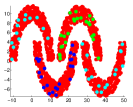
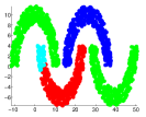
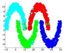
Figure 3: Segmentation for a random instance of the Four-Moons data set with $75$ labels produced by CSP (left), COSf (middle) and FAST-GE (right).

Figure 4: Accuracy and running times for the Four-Moons data set, where the underlying graph given by the model NoisyKnn($n=1500,k=30,l=15$), for varying number of constraints. Time is in logarithmic scale. The bars indicate the variance in the output over random trials using the same number of constraints.

PACM. Our second synthetic example is the somewhat more irregular PACM graph, formed by a cloud of $n=426$ points in the shape of letters $\{P,A,C,M\}$, whose topology renders the segmentation particularly challenging. The details about this data set are given in the section 10. Here we only present a visualization of the obtained segmentations.

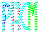
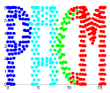
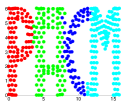
Figure 5: Top: Segmentation for a random instance of the PACM data set with $125$ labels produced by CSP (left), COSf (middle) and FAST-GE (right)

7.3 Image Data

In terms of real data, we consider two very different applications. Our first application is to segmentation of real images, where the underlying grid graph is given by the affinity matrix of the image, computed using the RBF kernel based on the grayscale values.

We construct the constraints by assigning cluster-membership information to a very small number of the pixels, which are shown colored in the pictures below. The cluster-membership information is then turned into pairwise constraints in the obvious way. Our output is obtained by running $k$-means 20 times and selecting the best segmentation according to the $k$-means objective value.

Patras. Figure 6 shows the 5-way segmentation of an image with approximately 44K pixels, which our method is able to detect in under 3 seconds. The size of this problem is prohibitive for CSP. The COSf algorithm runs in 40 seconds and while it does better on the lower part of the image it erroneously merges two of the clusters (the red and the blue one) into a single region.

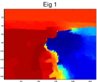
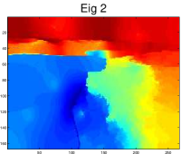
Figure 6: Patras: Top-left: Output of FAST-GE, in 2.8 seconds. Top-right: output of COSf, in 40.2 seconds. Bottom: heatmaps for the first two eigenvectors computed by FAST-GE.

Santorini. In Figure 7 we test our proposed method on the Santorini image, with approximately $250K$ pixels. Our approach successfully recovers a 4-way partitioning, with few errors, in just 15 seconds. Computing clusterings in data of this size is infeasible for CSP. The output of the COSf method, which runs in over 260 seconds, is meaningless.

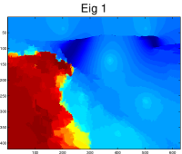
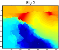
Figure 7: Santorini: Left: output of FAST-GE, in 15.2 seconds. Right: output of COSf, in 263.6 seconds. Bottom: heatmaps for the first two eigenvectors computed by FAST-GE.

Soccer. In Figure 8 we consider one last Soccer image, with approximately 1.1 million pixels. We compute a 5-way partitioning using the Fast-GE method in just 94 seconds. Note that while k-means clustering hinders some of the details in the image, the individual eigenvectors are able to capture finer details, such as the soccer ball for example, as shown in the two bottom plots of the same Figure 8. The output of the COSf method is obtained in 25 minutes and is again meaningless.

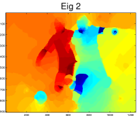
Figure 8: Top-right: output of FAST-GE, in under 94 seconds. Bottom-right: output of COSf in 25 minutes. Bottom-left: heat-maps of eigenvectors.

7.4 Friendship Networks

Our final data sets represent Facebook networks in American colleges. The work in [22] studies the structure of Facebook networks at one hundred American colleges and universities at a single point in time (2005) and investigate the community structure at each institution, as well as the impact and correlation of various self-identified user characteristics (such as residence, class year, major, and high school) with the identified network communities. While at many institutions, the community structures are organized almost exclusively according to class year, as pointed out in [21], other institutions are known to be organized almost exclusively according to its undergraduate House system (dormitory residence), which is very well reflected in the identified communities. It is thus a natural assumption to consider the dormitory affiliation as the ground truth clustering, and aim to recover this underlying structure from the available friendship graph and any available constraints. We add constraints to the clustering problem by sampling uniformly at random nodes in the graph, and the resulting pairwise constraints are generated depending on whether the two nodes belong to the same cluster or not. In order for us to be able to compare to the computationally expensive CSP method, we consider two small-sized schools, Simmons College ($n=850$, $\bar{d}=36$, $k=10$) and Haverford College ($n=1025$, $\bar{d}=72$, $k=15$), where $\bar{d}$ denotes the average degree in the graph and $k$ the number of clusters. For both examples, FAST-GE yields more accurate results than both CSP and COSf, and does so at a much smaller computational cost.

Figure 9: Facebook networks. Top: accuracy and running times for the Simmons College ($n=850$, $\bar{d}=36$, $k=10$). Bottom: accuracy and running times for Haverford College ($n=1025$, $\bar{d}=72$, $k=15$). Time is in logarithmic scale.

8 Final Remarks

We presented a spectral method that reduces constrained clustering into a generalized eigenvalue problem in which both matrices are Laplacians. This offers two advantages that are not simultaneously shared by any of the previous methods: an efficient implementation and an approximation guarantee for the 2-way partitioning problem in the form of a generalized Cheeger inequality. In practice this translates to a method that is at least 10x faster than some of the best existing algorithms, while producing output of superior quality. Its speed makes our method a good candidate for some type of iteration, e.g. as in [20], or interactive user feedback, that would further improve its output.

We view the Cheeger inequality we presented in section 6 as indicative of the rich mathematical properties of generalized Laplacian eigenvalue problems. We expect that tighter versions are to be discovered, along the lines of [11]. Finding $k$-way generalizations of the Cheeger inequality, as in [12], poses an interesting open problem.

9 Proof of the Generalized Cheeger Inequality

We begin with two Lemmas.

Lemma 9.1

For all $a_{i},b_{i}>0$ we have

$$\frac{\sum_{i}{a_{i}}}{\sum_{i}b_{i}}\geq\min_{i}\left\{\frac{a_{i}}{b_{i}}\right\}.$$

Lemma 9.2

Let $G$ be a graph, $d$ be the vector containing the degrees of the vertices, and $D$ be corresponding diagonal matrix. For all vectors $x$ where $x^{T}d=0$ we have

$$x^{T}Dx=x^{T}L_{D_{G}}x,$$

where $D_{G}$ is the demand graph for $G$.

Proof.

Let $d$ be the vector consisting of the entries along the diagonal of $D$. By definition, we have

$$L_{D_{G}}=D-\frac{dd^{T}}{vol(V)}.$$

The lemma follows. $\square$

We prove the following theorem.

Theorem 9.3

Let $G$ and $H$ be any two weighted graphs and $D$ be the vector containing the degrees of the vertices in $G$. F any vector $x$ such that $x^{T}d=0$, we have

$$\frac{x^{T}L_{G}x}{x^{T}L_{H}x}\geq\phi(G,D_{G})\cdot\phi(G,H)/4,$$

where $D_{G}$ is the demand graph of $G$. A cut meeting the guarantee of the inequality can be obtained via a Cheeger sweep on $x$.

Let $V^{-}$ denote the set of $u$ such that $x_{u}\leq 0$ and $V^{+}$ denote the set such that $x_{u}>0$. Then we can divide $E_{G}$ into two sets: $E_{G}^{same}$ consisting of edges with both endpoints in $V^{-}$ or $V^{+}$, and $E_{G}^{dif}$ consisting of edges with one endpoint in each. In other words:

$$E_{G}^{dif}=\delta_{G}\left(V^{-},V^{+}\right),\text{ and}$$

$$E_{G}^{same}=E_{G}\setminus E_{G}^{dif}.$$

We also define $E_{H}^{dif}$ and $E_{H}^{same}$ similarly.

We first show a lemma which is identical to one used in the proof of Cheeger's inequality [2]:

Lemma 9.4

Let $G$ and $H$ be any two weighted graphs on the same vertex set $V$ partitioned into $V^{-}$ and $V^{+}$. For any vector $x$ we have

$$\frac{\sum_{uv\in E_{G}^{same}}w_{G}\left(u,v\right)\left|x_{u}^{2}-x_{v}^{2}\right|+\sum_{uv\in E_{G}^{dif}}w_{G}(u,v)\left(x_{u}^{2}+x_{v}^{2}\right)}{x^{T}L_{H}x}\geq\frac{\phi(G,H)}{2}.$$

Proof.

We begin with a few algebraic identities:

Note that $2x_{u}^{2}+2x_{v}^{2}-(x_{u}-x_{v})^{2}=(x_{u}+x_{v})^{2}\geq 0$ gives:

$$\left(x_{u}-x_{v}\right)^{2}\leq 2x_{u}^{2}+2x_{v}^{2}.$$

Also, suppose $uv\in E_{H}^{same}$ and without loss of generality that $|x_{u}|\geq|x_{v}|$. Then letting $y=|x_{u}|-|x_{v}|$, we get:

$$|x_{u}^{2}-x_{v}^{2}| = \left(\left|x_{v}\right|+y\right)^{2}-\left|x_{v}\right|^{2}$$

$$= y^{2}+y|x_{v}|$$

$$\geq y^{2}=\left(x_{u}-x_{v}\right)^{2}.$$

The last equality follows because $x_{u}$ and $x_{v}$ have the same sign.

We then use the above inequalities to decompose the $x^{T}L_{H}x$ term.

$$x^{T}L_{H} = \sum_{uv\in E_{H}^{same}}w_{H}(u,v)\left(x_{u}-x_{v}\right)^{2}+\sum_{uv\in E_{H}^{dif}}w_{H}(u,v)\left(x_{u}-x_{v}\right)^{2}$$ (6)

$$\leq \sum_{uv\in E_{H}^{same}}w_{H}(u,v)\left(x_{u}-x_{v}\right)^{2}+\sum_{uv\in E_{H}^{dif}}w_{H}(u,v)\left(2x_{u}^{2}+2x_{v}^{2}\right)$$

$$\leq 2\left(\sum_{uv\in E_{H}^{same}}w_{H}(u,v)\left(x_{u}-x_{v}\right)^{2}+\sum_{uv\in E_{H}^{dif}}w_{H}(u,v)\left(x_{u}^{2}+x_{v}^{2}\right)\right)$$

$$\leq 2\left(\sum_{uv\in E_{H}^{same}}w_{H}(u,v)\left|x_{u}^{2}-x_{v}^{2}\right|+\sum_{uv\in E_{H}^{dif}}w_{H}(u,v)\left(x_{u}^{2}+x_{v}^{2}\right)\right).$$

We can now decompose the summation further into parts for $V^{-}$ and $V^{+}$:

$$\sum_{uv\in E_{G}^{same}}w_{G}\left(u,v\right)\left|x_{u}^{2}-x_{v}^{2}\right|+\sum_{uv\in E_{G}^{dif}}w_{G}\left(u,v\right)\left(x_{u}^{2}+x_{v}^{2}\right)$$

$$= \sum_{u\in V^{-},v\in V^{-}}w_{G}\left(u,v\right)\left|x_{u}^{2}-x_{v}^{2}\right|+\sum_{u\in V^{-},v\in V^{+}}w_{G}\left(u,v\right)x_{u}^{2}$$

$$+\sum_{u\in V^{+},v\in V^{+}}w_{G}\left(u,v\right)\left|x_{u}^{2}-x_{v}^{2}\right|+\sum_{u\in V^{-},v\in V^{+}}w_{G}\left(u,v\right)x_{u}^{2}.$$

Doing the same for $\sum_{uv\in E_{H}^{same}}w_{H}(u,v)|x_{u}^{2}-x_{v}^{2}|+\sum_{uv\in E_{H}^{dif}}w_{H}(u,v)(x_{u}^{2}+x_{v}^{2})$ we get:

$$\frac{\sum_{uv\in E_{G}^{same}}w_{G}(u,v)\left|x_{u}^{2}-x_{v}^{2}\right|+\sum_{uv\in E_{G}^{dif}}w_{G}(u,v)\left(x_{u}^{2}+x_{v}^{2}\right)}{x^{T}L_{H}x}$$

$$\geq \min\left\{\frac{\sum_{u\in V^{-},v\in V^{-}}w_{G}(u,v)\left|x_{u}^{2}-x_{v}^{2}\right|+\sum_{u\in V^{-},v\in V^{+}}w_{G}(u,v)x_{u}^{2}}{\sum_{u\in V^{-},v\in V^{-}}w_{H}(u,v)\left|x_{u}^{2}-x_{v}^{2}\right|+\sum_{u\in V^{-},v\in V^{+}}w_{H}(u,v)x_{u}^{2}},\right.$$

$$\qquad\left.\frac{\sum_{u\in V^{+},v\in V^{+}}w_{G}(u,v)\left|x_{u}^{2}-x_{v}^{2}\right|+\sum_{u\in V^{-},v\in V^{+}}w_{G}(u,v)x_{v}^{2}}{\sum_{u\in V^{+},v\in V^{+}}w_{H}(u,v)\left|x_{u}^{2}-x_{v}^{2}\right|+\sum_{u\in V^{-},v\in V^{+}}w_{H}(u,v)x_{v}^{2}}\right\}.$$

The inequality comes from applying of Lemma 9.1.

By symmetry in $V^{-}$ and $V^{+}$, it suffices to show that

$$\frac{\sum_{u\in V^{-},v\in V^{-}}w_{G}\left(u,v\right)\left|x_{u}^{2}-x_{v}^{2}\right|+\sum_{u\in V^{-},v\in V^{+}}w_{G}(u,v)x_{u}^{2}}{\sum_{u\in V^{-},v\in V^{-}}w_{G}\left(u,v\right)\left|x_{u}^{2}-x_{v}^{2}\right|+\sum_{u\in V^{-},v\in V^{+}}w_{G}\left(u,v\right)x_{u}^{2}}\geq\phi(G,H).\\$$ (7)

We sort the $x_{u}$ in increasing order of $|x_{u}|$ into such that $x_{u_{1}}\geq\ldots\geq x_{u_{k}}$, and let $S_{k}=\{x_{u_{1}},\ldots,x_{u_{k}}\}$. We have

$$\sum_{u\in V^{-},v\in V^{-}}w_{G}(u,v)\left|x_{u}^{2}-x_{v}^{2}\right|+\sum_{u\in V^{-},v\in V^{+}}w_{G}(u,v)x_{u}^{2}=\sum_{i=1\dots k}\left(x_{u_{i}}^{2}-x_{u_{i-1}}^{2}\right)cap_{G}\left(S_{k},\bar{S_{k}}\right),$$

and

$$\sum_{u\in V^{-},v\in V^{-}}w_{H}(u,v)\left|x_{u}^{2}-x_{v}^{2}\right|+\sum_{u\in V^{-},v\in V^{+}}w_{H}(u,v)x_{u}^{2}=\sum_{i=1\dots k}\left(x_{u_{i}}^{2}-x_{u_{i-1}}^{2}\right)cap_{H}\left(S_{k},\bar{S_{k}}\right).$$

Applying Lemma 9.1 we have

$$\frac{\sum_{u\in V^{-},v\in V^{-}}w_{G}(u,v)|x_{u}^{2}-x_{v}^{2}|+\sum_{u\in V^{-},v\in V^{+}}w_{G}(u,v)x_{u}^{2}}{\sum_{u\in V^{-},v\in V^{-}}w_{G}\left(u,v\right)\left|x_{u}^{2}-x_{v}^{2}\right|+\sum_{u\in V^{-},v\in V^{+}}w_{G}\left(u,v\right)x_{u}^{2}}\geq\min_{k}\frac{cap_{H}\left(S_{G},\bar{S_{i}}\right)}{cap_{H}\left(S_{i},\bar{S_{i}}\right)}\geq\phi(G,H),$$

where the second inequality is by definition of $\phi(G,H)$. This proves equation 7 and the Lemma follows. $\square$

We now proceed with the proof of the main Theorem.

Proof.

We have

$${x^{T}L_{G}x} = \sum_{uv\in E_{G}}w_{G}(u,v)(x_{u}-x_{v})^{2}$$

$$= \sum_{uv\in E_{G}^{same}}w_{G}(u,v)(x_{u}-x_{v})^{2}+\sum_{uv\in E_{G}^{dif}}w_{G}(u,v)(x_{u}-x_{v})^{2}$$

$$\geq \sum_{uv\in E_{G}^{same}}w_{G}(u,v)(x_{u}-x_{v})^{2}+\sum_{uv\in E_{G}^{dif}}w_{G}(u,v)(x_{u}^{2}+x_{v}^{2}).$$

The last inequality follows by $x_{u}x_{v}\leq 0$ as $x_{u}\leq 0$ for all $u\in V^{-}$ and $x_{v}\geq 0$ for all $v\in V^{+}$.

We multiply both sides of the inequality by

$$\sum_{uv\in E_{G}^{same}}w_{G}(u,v)(x_{u}+x_{v})^{2}+\sum_{uv\in E_{G}^{dif}}w_{G}(u,v)(x_{u}^{2}+x_{v}^{2}).$$

We have

$$\left(\sum_{uv\in E_{G}^{same}}w_{G}(u,v)(x_{u}-x_{v})^{2}+\sum_{uv\in E_{G}^{dif}}w_{G}(u,v)(x_{u}^{2}+x_{v}^{2})\right)$$

$$\cdot\left(\sum_{uv\in E_{G}^{same}}w_{G}(u,v)(x_{u}+x_{v})^{2}+\sum_{uv\in E_{G}^{dif}}w_{G}(u,v)(x_{u}^{2}+x_{v}^{2})\right)$$

$$\geq \left(\sum_{uv\in E_{G}^{same}}|x_{u}-x_{v}||x_{u}+x_{v}|+\sum_{uv\in E_{G}^{dif}}w_{G}(u,v)(x_{u}^{2}+x_{v}^{2})\right)^{2}$$

$$= \left(\sum_{uv\in E_{G}^{same}}|x_{u}^{2}-x_{v}^{2}|+\sum_{uv\in E_{G}^{dif}}w_{G}(u,v)(x_{u}^{2}+x_{v}^{2})\right)^{2}.$$

Furthermore, notice that $(x_{u}+x_{v})^{2}\leq 2x_{u}^{2}+2x_{v}^{2}$ since $2x_{u}^{2}+2x_{v}^{2}-(x_{u}+x_{v})^{2}=(x_{u}-x_{v})^{2}\geq 0$. So, we have

$$\sum_{uv\in E_{G}^{same}}w_{G}(u,v)(x_{u}+x_{v})^{2}+\sum_{uv\in E_{G}^{dif}}w_{G}(u,v)(x_{u}^{2}+x_{v}^{2})$$

$$\leq 2\left(\sum_{uv\in E_{G}^{same}}w_{G}(u,v)(x_{u}^{2}+x_{v}^{2})+\sum_{uv\in E_{G}^{dif}}w_{G}(u,v)(x_{u}^{2}+x_{v}^{2})\right)$$

$$=2x^{T}Dx\leq 4x^{T}L_{D_{G}}x,$$

where $D$ is the diagonal of $L_{G}$ and the last inequality comes from Lemma 9.2. Combining the last two inequalities we get:

$$\frac{x^{T}L_{G}x}{x^{T}L_{H}x}\geq \frac{1}{2}\cdot\left(\frac{\sum_{uv\in E_{G}^{same}}\left|x_{u}^{2}-x_{v}^{2}\right|+\sum_{uv\in E_{G}^{dif}}w_{G}(u,v)\left(x_{u}^{2}+x_{v}^{2}\right)}{x^{T}L_{H}x}\right)$$

$$\cdot\left(\frac{\sum_{uv\in E_{G}^{same}}\left|x_{u}^{2}-x_{v}^{2}\right|+\sum_{uv\in E_{G}^{dif}}w_{G}(u,v)\left(x_{u}^{2}+x_{v}^{2}\right)}{x^{T}L_{D_{G}}x}\right).$$

By Lemma 9.4, we have that the first factor is bounded by $\frac{1}{2}\phi(G,H)$ and the second factor bounded by $\frac{1}{2}\phi(G,D_{G})$. Hence we get

$$\frac{x^{T}L_{G}x}{x^{T}L_{H}x} \geq\frac{1}{4}\phi(G,H)\phi(G,{D_{G}}).$$ (9)

$\square$

10 Additional Experiments

PACM graph. We again consider the (very) noisy ensemble NoisyKnn($n=436,k_{g}=30,l_{g}=15$). Figure 10 shows a random instance of the clustering returned by each of the methods, with 125 constraints. Figure 11 shows the accuracy and running times of all three methods on this example. Again, our approach returns superior results when compared to CSP, and it is somewhat better than COSf. In this example, our running time is larger than that of both COSf and CSP, which is due to the small size of the problem ($n=426$). For such small problems a full eigenvalue decomposition is faster due to its better utilization of the FPU, as well as some overheads of the iterative method (e.g. preconditioning). In principle we can use the full eigenvalue decomposition to speed-up our algorithm for these smaller problems and at least match the performance of CSP. However the running times are already very small.

Figure 10: Top: Segmentation for a random instance of the PACM data set with $125$ labels produced by CSP (left), COSf (middle) and FAST-GE (right)

Figure 11: Leftmost plots illustrate the accuracy and running times for the Four-Moons data set, where the underlying graph given by the model NoisyKnn($n=1500,k=30,l=15$), for varying number of constraints. The rightmost two plots show similar statistics for the PACM data set, with the noise model given by NoisyKnn($n=426$, $k=30,l=15$). We average all results over 20 runs.

References

- [1] Sugato Basu, Ian Davidson, and Kiri Wagstaff. Constrained Clustering: Advances in Algorithms, Theory and Applications. CRC Press, 2008.
- [2] F.R.K. Chung. Spectral Graph Theory, volume 92 of Regional Conference Series in Mathematics. American Mathematical Society, 1997.
- [3] Anders P. Eriksson, Carl Olsson, and Fredrik Kahl. Normalized cuts revisited: A reformulation for segmentation with linear grouping constraints. Journal of Mathematical Imaging and Vision, 39(1):45–61, 2011.
- [4] G.H. Golub and C.F. Van Loan. Matrix Computations. The Johns Hopkins University Press, Baltimore, 3d edition, 1996.
- [5] Sepandar D. Kamvar, Dan Klein, and Christopher D. Manning. Spectral learning. In IJCAI-03, Proceedings of the Eighteenth International Joint Conference on Artificial Intelligence, Acapulco, Mexico, August 9-15, 2003, pages 561–566, 2003.
- [6] Jaya Kawale and Daniel Boley. Constrained spectral clustering using l1 regularization. In SDM, pages 103–111, 2013.
- [7] Andrew V. Knyazev. Toward the optimal preconditioned eigensolver: Locally optimal block preconditioned conjugate gradient method. SIAM J. Sci. Comput, 23:517–541, 2001.
- [8] Ioannis Koutis, Gary L. Miller, and Richard Peng. A nearly solver for SDD linear systems. In FOCS '11: Proceedings of the 52nd Annual IEEE Symposium on Foundations of Computer Science, 2011.
- [9] Ioannis Koutis, Gary L. Miller, and Richard Peng. A fast solver for a class of linear systems. Commun. ACM, 55(10):99–107, October 2012.
- [10] Ioannis Koutis, Gary L. Miller, and David Tolliver. Combinatorial preconditioners and multilevel solvers for problems in computer vision and image processing. Computer Vision and Image Understanding, 115(12):1638–1646, 2011.
- [11] Tsz Chiu Kwok, Lap Chi Lau, Yin Tat Lee, Shayan Oveis Gharan, and Luca Trevisan. Improved Cheeger's Inequality: Analysis of Spectral Partitioning Algorithms through Higher Order Spectral Gap. CoRR, abs/1301.5584, 2013.
- [12] James R. Lee, Shayan Oveis Gharan, and Luca Trevisan. Multi-way spectral partitioning and higher-order Cheeger inequalities. In Proceedings of the Forty-fourth Annual ACM Symposium on Theory of Computing, STOC '12, pages 1117–1130, New York, NY, USA, 2012. ACM.
- [13] Zhenguo Li, Jianzhuang Liu, and Xiaoou Tang. Constrained clustering via spectral regularization. In 2009 IEEE Computer Society Conference on Computer Vision and Pattern Recognition (CVPR 2009), 20-25 June 2009, Miami, Florida, USA, pages 421–428, 2009.
- [14] Zhengdong Lu and Miguel Á. Carreira-Perpiñán. Constrained spectral clustering through affinity propagation. In 2008 IEEE Computer Society Conference on Computer Vision and Pattern Recognition (CVPR 2008), 24-26 June 2008, Anchorage, Alaska, USA. IEEE Computer Society, 2008.
- [15] Andrew Y. Ng, Michael I. Jordan, and Yair Weiss. On spectral clustering: Analysis and an algorithm. In Advances in Neural Information Processing Systems 14 [Neural Information Processing Systems: Natural and Synthetic, NIPS 2001, December 3-8, 2001, Vancouver, British Columbia, Canada], pages 849–856, 2001.
- [16] W.M. Rand. Objective criteria for the evaluation of clustering methods. Journal of the American Statistical Association, 66(336):846–850, 1971.
- [17] Syama Sundar Rangapuram and Matthias Hein. Constrained 1-spectral clustering. In AISTATS, pages 1143–1151, 2012.
- [18] Jianbo Shi and Jitendra Malik. Normalized cuts and image segmentation. IEEE Trans. Pattern Anal. Mach. Intell., 22(8):888–905, 2000.
- [19] G.W. Stewart and Ji-Guang Sun. Matrix Perturbation Theory. Academic Press, Boston, 1990.
- [20] David Tolliver and Gary L. Miller. Graph partitioning by spectral rounding: Applications in image segmentation and clustering. In CVPR (1), pages 1053–1060, 2006.
- [21] Amanda L. Traud, Eric D. Kelsic, Peter J. Mucha, and Mason A. Porter. Comparing Community Structure to Characteristics in Online Collegiate Social Networks. SIAM Review, 53(3):526–543, August 2011.
- [22] Amanda L Traud, Peter J Mucha, and Mason A Porter. Social structure of Facebook networks. Physica A: Statistical Mechanics and its Applications, 2012.
- [23] Deepak Verma and Marina Meila. A comparison of spectral clustering algorithms. Technical report, 2003.
- [24] Xiang Wang, Buyue Qian, and Ian Davidson. Improving document clustering using automated machine translation. In Proceedings of the 21st ACM International Conference on Information and Knowledge Management, CIKM '12, pages 645–653, New York, NY, USA, 2012. ACM.
- [25] Xiang Wang, Buyue Qian, and Ian Davidson. On constrained spectral clustering and its applications. Data Min. Knowl. Discov., 28(1):1–30, 2014.
- [26] Linli Xu, Wenye Li, and Dale Schuurmans. Fast normalized cut with linear constraints. In 2009 IEEE Computer Society Conference on Computer Vision and Pattern Recognition (CVPR 2009), 20-25 June 2009, Miami, Florida, USA, pages 2866–2873, 2009.
- [27] Stella X. Yu and Jianbo Shi. Understanding popout through repulsion. In 2001 IEEE Computer Society Conference on Computer Vision and Pattern Recognition (CVPR 2001), with CD-ROM, 8-14 December 2001, Kauai, HI, USA, pages 752–757. IEEE Computer Society, 2001.
- [28] Stella X. Yu and Jianbo Shi. Segmentation given partial grouping constraints. IEEE Trans. Pattern Anal. Mach. Intell., 26(2):173–183, 2004.