Homoclinical Structure of Dynamic Equations on Time Scales

Abstract

Homoclinic and heteroclinic motions in dynamics equations on time scales is investigated. The utilized time scale is a specific one such that it is a union of disjoint compact intervals. A numerical example that supports the theoretical results is presented.

Keywords: Dynamic equations on time scales; Homoclinic and heteroclinic motions; Stable and unstable sets

1 Introduction

Dynamic equations on time scales has become one of the attractive subjects among mathematicians beginning with the studies of S. Hilger (1988). The theory of time scales has many applications in various disciplines such as mechanics, electronics, neural networks, population models and economics (Bohner & Peterson, 2001; Chen & Song, 2013; Tisdell & Zaidi, 2008; Zhang et al., 2010).

Homoclinic and heteroclinic motions play an important role in the theory of dynamical systems since they are concerned with the presence of chaos (Bertozzi, 1988; Chacon & Bejarano, 1995; Gonchenko et al., 1996; Shil’nikov, 1967; Wiggins, 1988). The existence of a homoclinic solution was obtained as a limit of periodic solutions in a second order non-autonomous Hamiltonian system on time scales in the paper (Su & Feng, 2014) by means of the mountain pass theorem and the standard minimizing argument. In the present paper, we consider differential equations on a specific time scale and show that perturbations through discrete equations give rise to the existence of homoclinic and heteroclinic motions in the system.

Let us denote by $\mathbb{R}$ and $\mathbb{Z}$ the sets of real numbers and integers, respectively. The basic concepts about differential equations on time scales are as follows (Bohner & Peterson, 2001; Lakshmikantham et al. 1996; Lakshmikantham & Vatsala, 2002; Lakshmikantham & Devi, 2006). A time scale is a nonempty closed subset of $\mathbb{R}.$ On a time scale $\mathbb{T}$, the forward and backward jump operators are defined as $\sigma(t)=\inf\left\{s\in\mathbb{T}:s>t\right\}$ and $\rho(t)=\sup\left\{s\in\mathbb{T}:s<t\right\},$ respectively. We say that a point $t\in\mathbb{T}$ is right-scattered if $\sigma(t)>t$ and right-dense if $\sigma(t)=t$. Similarly, if $\rho(t)<t,$ then $t\in\mathbb{T}$ is called left-scattered, and otherwise it is called left-dense. Besides, a function $h:\mathbb{T}\times\mathbb{R}^{n}\to\mathbb{R}^{n}$ is called rd-continuous if it is continuous at each $(t,u)\in\mathbb{T}\times\mathbb{R}^{n}$ with right-dense $t,$ and the limits $\displaystyle\lim_{(r,\nu)\to(t^{-},u)}h(r,\nu)=h(t-,u)$ and $\displaystyle\lim_{\nu\to u}h(t,\nu)=h(t,u)$ exist at each $(t,u)$ with left-dense $t.$ At a right-scattered point $t\in\mathbb{T},$ the $\Delta$-derivative of a continuous function $\vartheta$ is defined as $\vartheta^{\Delta}\left(t\right)=\displaystyle\frac{\vartheta\left(\sigma\left(t\right)\right)-\vartheta\left(t\right)}{\sigma\left(t\right)-t}.$ On the other hand, at a right-dense point $t,$ we have $\vartheta^{\Delta}\left(t\right)=\displaystyle\lim_{r\to t}\frac{\vartheta\left(t\right)-\vartheta\left(r\right)}{t-r}$ provided that the limit exists.

Let $\mathbb{T}_{0}$ be a time scale defined as $\mathbb{T}_{0}=\bigcup_{k=-\infty}^{\infty}[\theta_{2k-1},\theta_{2k}]$ in which $\left\{\theta_{k}\right\}_{k\in\mathbb{Z}}$ is a strictly increasing sequence of real numbers satisfying $\left|\theta_{k}\right|\to\infty$ as $\left|k\right|\to\infty.$ Suppose that there exist positive numbers $\bar{\kappa}$ and $\bar{\delta}$ such that $\theta_{2k}-\theta_{2k-1}\geq\bar{\kappa}$ and $\theta_{2k+1}-\theta_{2k}\leq\bar{\delta}$ for all $k\in\mathbb{Z}.$

In the present study, we consider the following equation,

$$y^{\Delta}(t)=Ay(t)+f(t,y(t))+g(t,\zeta),\ t\in\mathbb{T}_{0},$$ (1.1)

where $A$ is a constant $n\times n$ real valued matrix, the function $f:\mathbb{T}_{0}\times\mathbb{R}^{n}\to\mathbb{R}^{n}$ is rd-continuous and the function $g(t,\zeta)$ is defined through the equation $g(t,\zeta)=\zeta_{k}$ for $t\in[\theta_{2k-1},\theta_{2k}],$ $k\in\mathbb{Z},$ such that $\zeta=\left\{\zeta_{k}\right\}_{k\in\mathbb{Z}}$ is a sequence generated by the map

$$\zeta_{k+1}=F(\zeta_{k}),$$ (1.2)

where $\zeta_{0}\in\Lambda,$ $F:\Lambda\to\Lambda$ is a continuous function and $\Lambda$ is a bounded subset of $\mathbb{R}^{n}.$ We assume without loss of generality that $\theta_{-1}<0<\theta_{0}.$ Our aim in this paper is to show the existence of homoclinic and heteroclinic motions in the dynamics of system (1.1) in the case that the map (1.2) admits homoclinic and heteroclinic orbits.

The presence of chaos in systems of the form (1.1) was considered in the paper (Akhmet & Fen, 2015). The reduction technique to impulsive differential equations, which was presented by Akhmet and Turan (2006), was used in (Akhmet & Fen, 2015) to investigate the existence of chaos. The reader is referred to (Akhmet, 2009a, 2009b; Akhmet & Fen, 2012, 2013a, 2013b, 2014a, 2014b, 2016) for other chaos generation techniques in differential equations. In the literature, the generation of homoclinic and heteroclinic motions on the basis of functional spaces was first demonstrated in (Akhmet, 2008, 2010a). It was rigorously proved in (Akhmet, 2010a) that the chaotic attractors of relay systems contain homoclinic motions. By means of the structure of moments of impulses, similar results for differential equations with impacts were obtained in the study (Akhmet, 2008). On the other hand, taking advantage of perturbations, the presence of homoclinic and heteroclinic motions in impulsive differential equations was demonstrated in (Fen & Tokmak Fen, accepted), and an illustrative example concerning Duffing equations with impacts was provided. However, dynamic equations on time scales were not investigated in these papers. The novelty of the present study is the theoretical discussion of homoclinic and heteroclinic motions in dynamic equations on time scales. The definitions for the stable and unstable sets as well as homoclinic and heteroclinic motions on time scales are given on the basis of functional spaces. Simulations that support the theoretical results are also provided.

2 Preliminaries

Throughout the paper, the usual Euclidean norm for vectors and the norm induced by the Euclidean norm for square matrices (Horn & Johnson, 1992) will be utilized.

Let us take into account the function $\psi:\mathbb{T}^{\prime}_{0}\to\mathbb{R}$ defined as (Akhmet & Turan, 2006),

$$\displaystyle\psi(t)=\left\{\begin{array}[]{ll}\displaystyle t-\sum_{0<\theta_{2k}<t}\delta_{k},&t\geq 0,\\ \displaystyle t+\sum_{t\leq\theta_{2k}<0}\delta_{k},&t<0,\end{array}\right.$$

where $\delta_{k}=\theta_{2k+1}-\theta_{2k},$ $k\in\mathbb{Z},$ and $\mathbb{T}^{\prime}_{0}=\mathbb{T}_{0}\setminus\bigcup_{k=-\infty}^{\infty}\left\{\theta_{2k-1}\right\},$ and denote by $X(s,r)$ the transition matrix of the linear homogeneous impulsive system

$$\begin{array}[]{l}x^{\prime}(s)=Ax(s),~{}s\neq s_{k},\\ \Delta x|_{s=s_{k}}=\delta_{k}Ax(s_{k}),\end{array}$$

where $s_{k}=\psi(\theta_{2k}),$ $k\in\mathbb{Z},$ $\displaystyle\Delta x|_{s=s_{k}}=x(s_{k}+)-x(s_{k})$ and $\displaystyle x(s_{k}+)=\lim_{s\to s_{k}^{+}}x(s).$

The following conditions are required.

1. $\det(I+\delta_{k}A)\neq 0$ for all $k\in\mathbb{Z},$ where $I$ is the $n\times n$ identity matrix;

2. There exist positive numbers $N$ and $\lambda$ such that $\left\|X(s,r)\right\|\leq Ne^{-\lambda(s-r)}$ for $s\geq r;$

3. There exist positive numbers $M_{f}$ and $M_{F}$ such that $\displaystyle\sup_{t\in\mathbb{T}_{0},~{}y\in\mathbb{R}^{n}}\left\|f(t,y)\right\|\leq M_{f}$ and $\displaystyle\sup_{\upsilon\in\Lambda}\left\|F(\upsilon)\right\|\leq M_{F};$

4. There exists a positive number $L_{f}$ such that $\left\|f(t,y_{1})-f(t,y_{2})\right\|\leq L_{f}\left\|y_{1}-y_{2}\right\|$ for all $t\in\mathbb{T}_{0},$ $y_{1},y_{2}\in\mathbb{R}^{n}.$

5. $\displaystyle NL_{f}\left(\frac{1}{\lambda}+\frac{\bar{\delta}}{1-e^{-\lambda\bar{\kappa}}}\right)<1;$

6. $\displaystyle-\lambda+NL_{f}+\frac{1}{\bar{\kappa}}\ln\left(1+NL_{f}\bar{\delta}\right)<0.$

If the conditions $(C1)-(C5)$ are valid, then for a fixed solution $\zeta=\left\{\zeta_{k}\right\}_{k\in\mathbb{Z}}$ of (1.2) there exists a unique solution $\varphi_{\zeta}(t)$ of (1.1) which is bounded on $\mathbb{T}_{0}$ such that

$$\sup_{t\in\mathbb{T}_{0}}\left\|\varphi_{\zeta}(t)\right\|\leq N(M_{f}+M_{F})\Big{(}\displaystyle\frac{1}{\lambda}+\displaystyle\frac{\bar{\delta}}{1-e^{-\lambda\bar{\kappa}}}\Big{)}.$$

Moreover, if $(C6)$ additionally holds, then by using the Gronwall’s Lemma for piecewise continuous functions (Akhmet, 2010b; Samoilenko & Perestyuk, 1995) one can confirm that the bounded solution $\varphi_{\zeta}(t)$ attracts all other solutions of (1.1) for a fixed sequence $\zeta,$ that is, $\left\|y(t)-\varphi_{\zeta}(t)\right\|\to 0$ as $t\to\infty,$ $t\in\mathbb{T}_{0},$ where $y(t),$ $y(t^{0})=y_{0},$ is a solution of (1.1) for some $t^{0}\in\mathbb{T}_{0}$ and $y_{0}\in\mathbb{R}^{n}.$

In the next section, we will investigate the existence of homoclinic and heteroclinic motions in the dynamics of (1.1).

3 Homoclinic and Heteroclinic Motions

Denote by $\mathcal{H}$ the set of all sequences $\zeta=\left\{\zeta_{k}\right\}_{k\in\mathbb{Z}}$ obtained by the discrete map (1.2). The following definitions are adapted from the papers (Akhmet, 2008, 2010a).

The stable set of a sequence $\zeta\in\mathcal{H}$ is defined as

$$W^{s}(\zeta)=\left\{\eta=\left\{\eta_{k}\right\}_{k\in\mathbb{Z}}\in\mathcal{H}\ :\ \left\|\eta_{k}-\zeta_{k}\right\|\to 0~{}\textrm{as}~{}k\to\infty\right\},$$

and the unstable set of $\zeta$ is

$$W^{u}(\zeta)=\left\{\eta=\left\{\eta_{k}\right\}_{k\in\mathbb{Z}}\in\mathcal{H}\ :\ \left\|\eta_{k}-\zeta_{k}\right\|\to 0~{}\textrm{as}~{}k\to-\infty\right\}.$$

The set $\mathcal{H}$ is called hyperbolic if for each $\zeta\in\mathcal{H}$ the stable and unstable sets of $\zeta$ contain at least one element different from $\zeta.$ A sequence $\eta\in\mathcal{H}$ is homoclinic to another sequence $\zeta\in\mathcal{H}$ if $\eta\in W^{s}(\zeta)\cap W^{u}(\zeta).$ Moreover, $\eta\in\mathcal{H}$ is heteroclinic to the sequences $\zeta^{1},$ $\zeta^{2}\in\mathcal{H},$ $\eta\neq\zeta^{1},$ $\eta\neq\zeta^{2},$ provided that $\eta\in W^{s}(\zeta^{1})\cap W^{u}(\zeta^{2}).$

Suppose that $\mathcal{D}$ is the set consisting of all solutions $\varphi_{\zeta}(t),$ $\zeta\in\mathcal{H},$ of (1.1), which are bounded on $\mathbb{T}_{0}.$ A solution $\varphi_{\eta}(t)\in\mathcal{D}$ belongs to the stable set $W^{s}(\varphi_{\zeta}(t))$ of $\varphi_{\zeta}(t)\in\mathcal{D}$ if $\left\|\varphi_{\eta}(t)-\varphi_{\zeta}(t)\right\|\to 0$ as $t\to\infty,$ $t\in\mathbb{T}_{0}.$ Besides, $\varphi_{\eta}(t)$ is an element of the unstable set $W^{u}(\varphi_{\zeta}(t))$ of $\varphi_{\zeta}(t)$ provided that $\left\|\varphi_{\eta}(t)-\varphi_{\zeta}(t)\right\|\to 0$ as $t\to-\infty,$ $t\in\mathbb{T}_{0}.$

We say that $\mathcal{D}$ is hyperbolic if for each $\varphi_{\zeta}(t)\in\mathcal{D}$ the sets $W^{s}(\varphi_{\zeta}(t))$ and $W^{u}(\varphi_{\zeta}(t))$ contain at least one element different from $\varphi_{\zeta}(t).$ A solution $\varphi_{\eta}(t)\in\mathcal{D}$ is homoclinic to another solution $\varphi_{\zeta}(t)\in\mathcal{D}$ if $\varphi_{\eta}(t)\in W^{s}(\varphi_{\zeta}(t))\cap W^{u}(\varphi_{\zeta}(t)),$ and $\varphi_{\eta}(t)\in\mathcal{D}$ is heteroclinic to the bounded solutions $\varphi_{\zeta^{1}}(t),$ $\varphi_{\zeta^{2}}(t)\in\mathcal{D},$ $\varphi_{\eta}(t)\neq\varphi_{\zeta^{1}}(t),$ $\varphi_{\eta}(t)\neq\varphi_{\zeta^{2}}(t),$ if $\varphi_{\eta}(t)\in W^{s}(\varphi_{\zeta^{1}}(t))\cap W^{u}(\varphi_{\zeta^{2}}(t)).$

The following theorem can be proved by using the reduction technique to impulsive differential equations, which was introduced in (Akhmet & Turan, 2006).

Theorem 3.1

Under the conditions $(C1)-(C6),$ the following assertions are valid:

1. If $\eta\in\mathcal{H}$ is homoclinic to $\zeta\in\mathcal{H},$ then $\varphi_{\eta}(t)\in\mathcal{D}$ is homoclinic to $\varphi_{\zeta}(t)\in\mathcal{D};$

2. If $\eta\in\mathcal{H}$ is heteroclinic to $\zeta^{1},$ $\zeta^{2}\in\mathcal{H},$ then $\varphi_{\eta}(t)\in\mathcal{D}$ is heteroclinic to $\varphi_{\zeta^{1}}(t),$ $\varphi_{\zeta^{2}}(t)\in\mathcal{D};$

3. If $\mathcal{H}$ is hyperbolic, then the same is true for $\mathcal{D}.$

The next section is devoted to a numerical example, which supports the results of Theorem 3.1.

4 An Example

Consider the following system,

$$\begin{array}[]{l}y_{1}^{\Delta}(t)=\displaystyle-(11/60)y_{1}(t)+(1/30)y_{2}(t)+0.05\sin\left(\pi t/4\right)+g(t,\zeta),\\ y_{2}^{\Delta}(t)=\displaystyle-(1/20)y_{1}(t)-(1/15)y_{2}(t)+0.003\arctan(y_{1}(t)),\end{array}$$ (4.7)

where $t$ belongs to the time scale $\mathbb{T}_{0}=\bigcup_{k=-\infty}^{\infty}[\theta_{2k-1},\theta_{2k}],$ $\theta_{k}=4k+(5+(-1)^{k})/2$ and $g(t,\zeta)=\zeta_{k}$ for $t\in[\theta_{2k-1},\theta_{2k}],$ $k\in\mathbb{Z},$ such that $\zeta=\left\{\zeta_{k}\right\}_{k\in\mathbb{Z}},$ $\zeta_{0}\in[0,1],$ is a sequence generated by the logistic map

$$\zeta_{k+1}=F(\zeta_{k}),$$ (4.8)

where $F(\upsilon)=3.9\upsilon(1-\upsilon).$ It is worth noting that the map (4.8) is chaotic in the sense of Li-Yorke (Li & Yorke, 1975), and the unit interval $[0,1]$ is invariant under the iterations of the map (Hale & Koçak, 1991).

System (4.7) is in the form of (1.1), where

$$A=\left(\begin{array}[]{ccc}-\displaystyle\frac{11}{60}&\displaystyle\frac{1}{30}\\ \vskip 6.0pt plus 2.0pt minus 2.0pt\cr-\displaystyle\frac{1}{20}&-\displaystyle\frac{1}{15}\end{array}\right),\ \ f(t,y_{1},y_{2})=\left(\begin{array}[]{ccc}0.05\displaystyle\sin\left(\frac{\pi}{4}t\right)\\ \vskip 6.0pt plus 2.0pt minus 2.0pt\cr 0.003\arctan(y_{1})\end{array}\right).$$

The conditions $(C1)-(C6)$ are valid for system (4.7) with $N=2.62,$ $\lambda=1/12,$ $M_{f}=0.0503,$ $L_{f}=0.003,$ $\bar{\kappa}=5$ and $\bar{\delta}=3.$

Since $t+8\in\mathbb{T}_{0}$ whenever $t\in\mathbb{T}_{0}$ and $f(t+8,y_{1},y_{2})=f(t,y_{1},y_{2})$ for all $t\in\mathbb{T}_{0},$ $y_{1},$ $y_{2}\in\mathbb{R},$ system (4.7) is Li-Yorke chaotic according to the results of (Akhmet & Fen, 2015). Moreover, one can verify that if $\zeta=\left\{\zeta_{k}\right\}_{k\in\mathbb{Z}}$ is a $p$-periodic solution of (4.8) for some natural number $p,$ then the corresponding bounded solution $\varphi_{\zeta}(t)$ of (4.7) is $8p$-periodic. The $y_{1}$ and $y_{2}$ coordinates of the solution of (4.7) with $y_{1}(0)=3,$ $y_{2}(0)=-2,$ $\zeta_{0}=0.292$ is shown in Figure 1. It is seen in Figure 1 that the solution behaves chaotically.

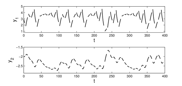
Figure 1: The solution of (4.7) corresponding to the initial data $y_{1}(0)=3,$ $y_{2}(0)=-2,$ $\zeta_{0}=0.292.$ The figure confirms the presence of chaos in system (4.7).

Now, we will demonstrate that homoclinic and heteroclinic motions take place in the chaotic dynamics of (4.7). Consider the function $\gamma_{1}(\upsilon)=\displaystyle\frac{1}{2}\left(1+\sqrt{1-\frac{4\upsilon}{3.9}}\right).$ It was mentioned in (Avrutin et al., 2015) that the orbit

$$\eta=\left\{\ldots,\gamma^{3}_{1}(\eta_{0}),\gamma_{1}^{2}(\eta_{0}),\gamma_{1}(\eta_{0}),\eta_{0},F(\eta_{0}),F^{2}(\eta_{0}),F^{3}(\eta_{0}),\ldots\right\},$$

where $\eta_{0}=1/3.9,$ is homoclinic to the fixed point $\eta^{*}=2.9/3.9$ of (4.8). Denote by $\varphi_{\eta}(t)$ and $\varphi_{\eta^{*}}(t)$ the bounded solutions of (4.7) corresponding to $\eta$ and $\eta^{*},$ respectively. Theorem 3.1 implies that $\varphi_{\eta}(t)$ is homoclinic to $\varphi_{\eta^{*}}(t).$ Notice that the bounded solution $\varphi_{\eta^{*}}(t)$ is $8$-periodic. We depict in Figure 2 the $y_{2}$ coordinates of $\varphi_{\eta}(t)$ and $\varphi_{\eta^{*}}(t).$ Figure 2 supports the result of Theorem 3.1 such that $\varphi_{\eta}(t)$ is homoclinic to $\varphi_{\eta^{*}}(t).$

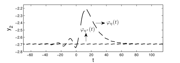
Figure 2: The homoclinic solution of (4.7). The simulation demonstrates that $\left\|\varphi_{\eta}(t)-\varphi_{\eta^{*}}(t)\right\|\to 0$ as $t\to\pm\infty,$ $t\in\mathbb{T}_{0}.$

On the other hand, the orbit

$$\overline{\eta}=\left\{\ldots,\gamma^{3}_{2}(\overline{\eta}_{0}),\gamma_{2}^{2}(\overline{\eta}_{0}),\gamma_{2}(\overline{\eta}_{0}),\overline{\eta}_{0},F(\overline{\eta}_{0}),F^{2}(\overline{\eta}_{0}),F^{3}(\overline{\eta}_{0}),\ldots\right\},$$

where the function $\gamma_{2}$ is defined as $\gamma_{2}(\upsilon)=\displaystyle\frac{1}{2}\left(1-\sqrt{1-\frac{4\upsilon}{3.9}}\right)$ and $\overline{\eta}_{0}=1/3.9,$ is heteroclinic to the fixed points $\eta^{*}=2.9/3.9$ and $\eta^{**}=0$ of (4.8) according to the results of (Avrutin et al., 2015). Suppose that $\varphi_{\overline{\eta}}(t),$ $\varphi_{\eta^{*}}(t)$ and $\varphi_{\eta^{**}}(t)$ are the bounded solutions of (4.7) corresponding to the sequences $\overline{\eta},$ $\eta^{*}$ and $\eta^{**},$ respectively. One can confirm by using Theorem 3.1 that the solution $\varphi_{\overline{\eta}}(t)$ is heteroclinic to $\varphi_{\eta^{*}}(t),$ $\varphi_{\eta^{**}}(t).$ The $y_{2}$ coordinates of $\varphi_{\overline{\eta}}(t),$ $\varphi_{\eta^{*}}(t)$ and $\varphi_{\eta^{**}}(t)$ are represented in Figure 3, which reveals that $\left\|\varphi_{\overline{\eta}}(t)-\varphi_{\eta^{*}}(t)\right\|\to 0$ as $t\to\infty,$ $t\in\mathbb{T}_{0}$ and $\left\|\varphi_{\overline{\eta}}(t)-\varphi_{\eta^{**}}(t)\right\|\to 0$ as $t\to-\infty,$ $t\in\mathbb{T}_{0}.$

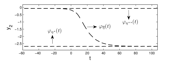
Figure 3: The heteroclinic solution of (4.7). It is observable that the bounded solution $\varphi_{\overline{\eta}}(t)$ is heteroclinic to the $8$-periodic solutions $\varphi_{\eta^{*}}(t),$ $\varphi_{\eta^{**}}(t).$

5 Conclusion

The present study is devoted to the existence of homoclinic and heteroclinic motions in dynamic equations on time scales. Sufficient conditions that guarantee the existence of homoclinic and heteroclinic motions are provided, and the definitions of stable and unstable sets are given on the basis of functional spaces. The equation under investigation can be considered as a hybrid system since it combines the dynamics of the discrete map with the continuous dynamics of the equation on time scales. The presented example and simulations reveal the applicability of our theoretical results.

References

• [1] M. U. Akhmet and M. Turan, The differential equations on time scales through impulsive differential equations, Nonlinear Analysis, 65 (2006) 2043-2060.
• [2] M. U. Akhmet, Hyperbolic sets of impact systems, Dyn. Contin. Discrete Impuls. Syst. Ser. A Math. Anal., 15 (Suppl. S1) (2008) 1-2, in: Proceedings of the $5$th International Conference on Impulsive and Hybrid Dynamical Systems and Applications, Beijing, Watan Press, 2008.
• [3] M. U. Akhmet, Devaney’s chaos of a relay system, Commun. Nonlinear Sci. Numer. Simulat., 14 (2009a), 1486-1493.
• [4] M. U. Akhmet, Li-Yorke chaos in the system with impacts, J. Math. Anal. Appl., 351 (2009b) 804-810.
• [5] M. U. Akhmet, Homoclinical structure of the chaotic attractor, Commun. Nonlinear Sci. Numer. Simulat., 15 (2010a) 819-822.
• [6] M. Akhmet, Principles of Discontinuous Dynamical Systems, Springer, New York, 2010b.
• [7] M. U. Akhmet and M. O. Fen, Chaotic period-doubling and OGY control for the forced Duffing equation, Commun. Nonlinear Sci. Numer. Simulat., 17 (2012) 1929-1946.
• [8] M. U. Akhmet and M. O. Fen, Replication of chaos, Commun. Nonlinear Sci. Numer. Simulat., 18 (2013a) 2626-2666.
• [9] M. U. Akhmet and M. O. Fen, Shunting inhibitory cellular neural networks with chaotic external inputs, Chaos, 23 (2013b) 023112.
• [10] M. U. Akhmet and M. O. Fen, Entrainment by chaos, Journal of Nonlinear Science, 24 (2014a) 411-439.
• [11] M. U. Akhmet and M. O. Fen, Replication of discrete chaos, Chaotic Modeling and Simulation (CMSIM), 2 (2014b) 129-140.
• [12] M. Akhmet and M. O. Fen, Li-Yorke chaos in hybrid systems on a time scale, Int. J. Bifurcat. Chaos, 25 (2015) 1540024.
• [13] M. Akhmet and M. O. Fen, Replication of Chaos in Neural Networks, Economics and Physics, Springer-Verlag, Berlin, Heidelberg, 2016.
• [14] V. Avrutin, B. Schenke, and L. Gardini, Calculation of homoclinic and heteroclinic orbits in 1D maps, Commun. Nonlinear Sci. Numer Simulat., 22 (2015) 1201-1214.
• [15] A. L. Bertozzi, Heteroclinic orbits and chaotic dynamics in planar fluid flows, Siam J. Math. Anal., 19 (1988) 1271-1294.
• [16] M. Bohner and A. Peterson, Dynamic Equations on Time Scales: An Introduction with Applications, Birkhäuser, Boston, 2001.
• [17] R. Chacon and J. D. Bejarano, Homoclinic and heteroclinic chaos in a triple-well oscillator, Journal of Sound and Vibration, 186 (1995) 269-278.
• [18] X. Chen and Q. Song, Global stability of complex-valued neural networks with both leakage time delay and discrete time delay on time scales, Neurocomputing, 121 (2013) 254-264.
• [19] M. O. Fen and F. Tokmak Fen, Homoclinic and heteroclinic motions in hybrid systems with impacts, Math. Slovaca (accepted).
• [20] S. V. Gonchenko, L.P. Shil’nikov, and D.V. Turaev, Dynamical phenomena in systems with structurally unstable Poincaré homoclinic orbits, Chaos, 6 (1996) 15-31.
• [21] J. Hale and H. Koçak, Dynamics and Bifurcations, Springer-Verlag, New York, 1991.
• [22] S. Hilger, Ein Maßkettenkalkül mit Anwendung auf Zentrumsmanningfaltigkeiten, PhD Thesis, Universität Würzburg, 1988.
• [23] R. A. Horn and C. R. Johnson, Matrix Analysis, Cambridge University Press, United States of America, 1992.
• [24] V. Lakshmikantham, S. Sivasundaram, and B. Kaymakcalan, Dynamic Systems on Measure Chains, Kluwer Academic Publishers, Netherlands, 1996.
• [25] V. Lakshmikantham and A. S. Vatsala, Hybrid systems on time scales, J. Comput. Appl. Math., 141 (2002) 227-235.
• [26] V. Lakshmikantham and J. V. Devi, Hybrid systems with time scales and impulses, Nonlinear Analysis, 65 (2006) 2147-2152.
• [27] T.-Y. Li and J. A. Yorke, Period three implies chaos, The American Mathematical Monthly, 82 (1975) 985-992.
• [28] A. M. Samoilenko and N. A. Perestyuk, Impulsive Differential Equations, World Scientific, Singapore, 1995.
• [29] L. P. Shil’nikov, On a Poincaré-Birkhoff problem, Math. USSR-Sbornik, 3 (1967) 353-371.
• [30] Y. Su and Z. Feng, Homoclinic orbits and periodic solutions for a class of Hamiltonian systems on time scales, J. Math. Anal. Appl., 411 (2014) 37-62.
• [31] C. C. Tisdell and A. Zaidi, Basic qualitative and quantitative results for solutions to nonlinear, dynamic equations on time scales with an application to economic modelling, Nonlinear Analysis, 68 (2008) 3504-3524.
• [32] S. Wiggins, Global Bifurcations and Chaos: Analytical Methods, Springer-Verlag, New York, 1988.
• [33] J. Zhang, M. Fan, and H. Zhu, Periodic solution of single population models on time scales, Mathematical and Computer Modelling, 52 (2010) 515-521.