$A_{\infty}$ functors for Lagrangian correspondences

Abstract.

We construct $A_{\infty}$ functors between Fukaya categories associated to monotone Lagrangian correspondences between compact symplectic manifolds. We then show that the composition of $A_{\infty}$ functors for correspondences is homotopic to the functor for the composition, in the case that the composition is smooth and embedded.

1. Introduction

Recall that to any compact symplectic manifold $(M,\omega)$ satisfying suitable monotonicity conditions is a Fukaya category ${\operatorname{Fuk}}(M)$ whose objects are Lagrangian submanifolds, morphism spaces are Lagrangian Floer cochain groups, and composition maps count pseudoholomorphic polygons with boundary in a given sequence of Lagrangians [10]. A construction of Kontsevich [16] constructs a triangulated derived Fukaya category which is related via the homological mirror symmetry conjecture to the derived category of bounded complexes of coherent sheaves. The latter admits natural Mukai functors associated to correspondences which play an important role in, for example, the McKay correspondence [27], the work of Nakajima [23], etc.

The main result of this paper constructs $A_{\infty}$ functors associated to monotone Lagrangian correspondences which are meant to be mirror analogs to the Mukai functors. We learned the idea of constructing functors associated to Lagrangian correspondences from Fukaya, who suggested an approach using duality. In his construction the functor maps a Fukaya category of the domain of the correspondence to the dual of the codomain.. This makes composition of functors problematic; the approach here avoids that problem by enlarging the Fukaya category. The results of this paper are chain-level versions of an earlier paper [42] in which the second two authors constructed cohomology-level functors between categories for Lagrangian correspondences. We also showed in [43] that composition of these functors agrees with the geometric composition in the case that the Lagrangian correspondences have embedded composition. Applications of the calculus of $A_{\infty}$ functors developed in this paper can be found in Abouzaid and Smith [1] and Smith [32], as well as in Wehrheim-Woodward [39], [40], [35].

1.1. Summary of results

Given $A_{\infty}$ categories $\mathcal{C}_{0},\mathcal{C}_{1},$ let $\operatorname{Func}(\mathcal{C}_{0},\mathcal{C}_{1})$ denote the $A_{\infty}$ category of functors from $\mathcal{C}_{0}$ to $\mathcal{C}_{1}$ (see Definition 8.1 for our conventions on $A_{\infty}$ categories and functors). We construct for any pair of monotone symplectic manifolds $M_{0},M_{1}$ a Fukaya category of admissible correspondences ${\operatorname{Fuk}^{\includegraphics[height=5.05942pt]{sharp.eps}}}(M_{0},M_{1})$. The objects of ${\operatorname{Fuk}^{\includegraphics[height=5.05942pt]{sharp.eps}}}(M_{0},M_{1})$ are sequences of compact Lagrangian correspondences with a brane structure, which we call generalized Lagrangian correspondences. The brane structure consists of an orientation, grading, and relative spin structure. The correspondences are also required to be admissible in the sense that the minimal Maslov numbers are at least three, or vanishing disk invariant, and the fundamental groups are torsion for any choice of base point. Denote by ${\operatorname{Fuk}^{\includegraphics[height=5.05942pt]{sharp.eps}}}(M):={\operatorname{Fuk}^{\includegraphics[height=5.05942pt]{sharp.eps}}}(\operatorname{pt},M)$ the natural enlargement of the Fukaya category ${\operatorname{Fuk}}(M)$ whose objects are admissible generalized Lagrangian correspondences with brane structures from points to a compact monotone symplectic manifold $M$. Our first main result is:

Theorem 1.1.

(Functors for Lagrangian correspondences) Suppose that $M_{0},M_{1}$ are compact monotone symplectic manifolds with the same monotonicity constant. There exists an $A_{\infty}$ functor

$${\operatorname{Fuk}^{\includegraphics[height=5.05942pt]{sharp.eps}}}(M_{0},M_{1})\to\operatorname{Func}({\operatorname{Fuk}^{\includegraphics[height=5.05942pt]{sharp.eps}}}(M_{0}),{\operatorname{Fuk}^{\includegraphics[height=5.05942pt]{sharp.eps}}}(M_{1}))$$

inducing the functor of cohomology categories in [42, Definition 5.1].

In particular, for each admissible Lagrangian correspondence $L_{01}\subset M_{0}^{-}\times M_{1}$ equipped with a brane structure we construct an $A_{\infty}$ functor

$$\Phi(L_{01}):{\operatorname{Fuk}^{\includegraphics[height=5.05942pt]{sharp.eps}}}(M_{0})\to{\operatorname{Fuk}^{\includegraphics[height=5.05942pt]{sharp.eps}}}(M_{1})$$

acting in the expected way on Floer cohomology: for Lagrangian branes $L_{0}\subset M_{0},L_{1}\subset M_{1}$ there is an isomorphism with $\mathbb{Z}_{2}$-coefficients

$$H\operatorname{Hom}(\Phi(L_{01})L_{0},L_{1})\cong HF(L_{0}^{-}\times L_{1},L_{01})$$

where the right-hand-side is the Floer cohomology of the pair $(L_{0}^{-}\times L_{1},L_{01})$. For a pair of Lagrangian correspondences $L_{01},L_{01}^{\prime}\in M_{0}^{-}\times M_{1}$ and a Floer cocycle $\alpha\in CF(L_{01},L_{01}^{\prime})$ we construct a natural transformation

$$\mathcal{T}_{\alpha}:\Phi(L_{01})\to\Phi(L_{01}^{\prime})$$

of the corresponding $A_{\infty}$ functors.

The behavior of the $A_{\infty}$ functors for Lagrangian correspondences under embedded geometric composition as defined in [43] is our second main result. To state it, we recall that the geometric composition of Lagrangian correspondences

$$L_{01}\subset M_{0}^{-}\times M_{1},\quad L_{12}\subset M_{1}^{-}\times M_{2}$$

is

(1) $$L_{01}\circ L_{12}:=\pi_{02}(L_{01}\times_{M_{1}}L_{12})$$

where $\pi_{02}:M_{0}\times M_{1}^{2}\times M_{2}\to M_{0}\times M_{2}$ is the projection onto the product of the first and last factors. If the fiber product is transverse and embedded by $\pi_{02}$ then $L_{01}\circ L_{12}$ is a smooth Lagrangian correspondence.

Theorem 1.2.

(Geometric composition theorem) Suppose that $M_{0},M_{1},M_{2}$ are monotone symplectic manifolds with the same monotonicity constant. Let $L_{01}\subset M_{0}^{-}\times M_{1},L_{12}\subset M_{1}^{-}\times M_{2}$ be admissible Lagrangian correspondences with spin structures and gradings such that $L_{01}\circ L_{12}$ is smooth, embedded by $\pi_{02}$ in $M_{0}^{-}\times M_{2}$, and admissible. Then there exists a homotopy of $A_{\infty}$ functors

$$\Phi(L_{12})\circ\Phi(L_{01})\simeq\Phi(L_{01}\circ L_{12}).$$

There is a slightly more complicated statement in the case that the correspondences are only relatively spin, which involves a shift in the background class. In particular, the theorem implies that the associated derived functors

$$D(\Phi(L_{12}))\circ D(\Phi(L_{01}))\cong D(\Phi(L_{01}\circ L_{12})):D{\operatorname{Fuk}^{\includegraphics[height=5.05942pt]{sharp.eps}}}(M_{0})\to D{\operatorname{Fuk}^{\includegraphics[height=5.05942pt]{sharp.eps}}}(M_{2})$$

are canonically isomorphic. The result extends to generalized Lagrangian correspondences, in particular the empty correspondence. In the last case the result shows that the Fukaya categories constructed using two different systems of perturbation data are homotopy equivalent.

A complete chain-level version of the earlier work is still missing. Namely, one would like to construct a Weinstein-Fukaya $A_{\infty}$ $2$-category whose objects are symplectic manifolds and morphism categories are the extended Fukaya categories of correspondences. Furthermore one would like an $A_{\infty}$ categorification functor given by the extended Fukaya categories on objects and the functor of Theorem 1.1 on morphisms. This theory would be the chain level version of the Weinstein-Floer $2$-category and categorification functor constructed in [42]. Some steps in this direction have been taken by Bottman [5], [6]. Batanin has pointed out to us a possibly-relevant construction of homotopy higher categories in [2, Definition 8.7].

The $A_{\infty}$ structures, functors, and natural transformations are defined using a general theory of family quilt invariants that count pseudoholomorphic quilts with varying domain. This theory includes families of quilts associated to the associahedron, multiplihedron, and other polytopes underlying the various $A_{\infty}$ structures. Unfortunately these families of quilted surfaces come with the rather inconvenient (for analysis) property that degeneration is not given by “neck stretching” but rather by “nodal degeneration”. Our first step is to replace these families by ones that are more analytically convenient, see Section 2 for the precise definitions. We say that a stratified space is labelled by quilt data if for each stratum there is given a combinatorial type of quilted surface, and each pair of strata there is given a subset of gluing parameters for the strip like ends as in Definition 2.17 below. For technical reasons (contractibility of various choices) it is helpful to restrict to the case that each patch of each quilt is homeomorphic to a disk with at least one marking, and so has homotopically trivial automorphism group. Such quilt data are called irrotatable; the general case could be handled with more complicated data associated to the stratified space.

Theorem 1.3.

(Existence of families of quilts with strip-like ends) Given a stratified space $\mathcal{R}$ equipped with irrotatable quilt data, then there exists a family of quilted surfaces $\SS=(\underline{S}_{r})_{r\in\mathcal{R}}$ with strip-like ends over $\mathcal{R}$ with the given data in which degeneration is given by neck-stretching.

The next step is to define pseudoholomorphic quilt invariants associated to these families. Let $\SS=(\underline{S}_{r},r\in\mathcal{R})$ be a family of quilted surfaces with strip-like ends over a stratified space $\mathcal{R}$, $\underline{M}$ be a collection of admissible monotone symplectic manifolds associated to the patches, and $\underline{L}$ a collection of admissible monotone Lagrangian correspondences associated to the seams and boundary components. Given a family $\underline{J}$ of compatible almost complex structures on the collection $\underline{M}$ and a Hamiltonian perturbation $\underline{K}$, a holomorphic quilt from a fiber of $\SS$ to $\underline{M}$ is pair

$$(r\in\mathcal{R},\underline{u}:\underline{S}_{r}\to\underline{M})$$

consisting of a point $r\in\mathcal{R}$ together with a $(\underline{J},\underline{K})$-holomorphic map $\underline{u}:\underline{S}_{r}\to\underline{M}$ taking values in $\underline{L}$ on the seams and boundary, see Definition 3.2 for the precise equation. The necessary regularity statement is the following, proved in Theorem 3.4 in Section 2.

Theorem 1.4.

(Transversality for families of holomorphic quilts) Suppose that $\SS\to\mathcal{R}$ is a family of quilted surfaces with strip-like ends equipped with compact monotone symplectic manifolds $\underline{M}$ for the patches and admissible Lagrangian correspondences $\underline{L}$ for the seams/boundaries. Suppose over the boundary of $\mathcal{R}$ a collection of perturbation data $(\underline{J},\underline{K})$ is given making all pseudoholomorphic quilts of formal dimension at most one regular. Then for a generic extension of $(\underline{J},\underline{K})$ agreeing with the extensions given by gluing near the boundary $\SS|_{\partial\mathcal{R}}$, every pseudoholomorphic quilt $u:\underline{S}_{r}\to\underline{M}$ of formal dimension at most one with strip-like ends is parametrized regular.

Using Theorem 1.4 we construct moduli spaces of pseudoholomorphic quilts and, using these, chain level family quilt invariants given as counts of isolated elements in the moduli space. As in the standard topological field theory philosophy, these invariants map the tensor product of cochain groups for the incoming ends $\mathcal{E}_{-}(\SS)$ to that for the outgoing ends $\mathcal{E}_{+}(\SS)$:

$$\Phi_{\SS}:\bigotimes_{\underline{e}\in\mathcal{E}_{-}(\SS)}CF(\underline{L}_{\underline{e}})\to\bigotimes_{\underline{e}\in\mathcal{E}_{+}(\SS)}CF(\underline{L}_{\underline{e}}).$$

These chain-level family invariants satisfy a master equation arising from the study of one-dimension components of the moduli spaces of pairs above:

Theorem 1.5.

(Master equation for family quilt invariants) Suppose that, in the setting of Theorem 1.4, $\SS\to\mathcal{R}$ is a family of quilted surfaces with strip-like ends over an oriented stratified space $\mathcal{R}=\cup_{\Gamma}\mathcal{R}_{\Gamma}$ (here the strata are indexed by $\Gamma$) with boundary multiplicities $m_{\Gamma}\in\mathbb{Z},\operatorname{codim}(\mathcal{R}_{\Gamma})=1$. Then the chain level invariant $\Phi_{\SS}$ and the coboundary operators $\partial$ on the tensor products of Floer cochain complexes satisfy the relation

$$\partial\circ\Phi_{\SS}-\Phi_{\SS}\circ\partial=\sum_{\Gamma,\operatorname{codim}(\mathcal{R}_{\Gamma})=1}m_{\Gamma}\Phi_{\SS_{\Gamma}}.$$

In other words, if $\partial\SS$ denotes the contribution from boundary components of $\mathcal{R}$ counted with multiplicity and $\partial\Phi_{\SS}=[\partial,\Phi_{\SS}]$ denotes the boundary of $\Phi_{\SS}$ considered as a morphism of chain complexes then

(2) $$\partial\Phi_{\SS}=\Phi_{\partial\SS}.$$

The master equation (2) specializes to the $A_{\infty}$ associativity, functor, natural transformation, and homotopy axioms for the various families of quilts we consider.

The paper is divided into two parts. The first part covers the general theory of parametrized pseudoholomorphic quilts and the construction of family quilt invariants. The second part covers the application of this general theory to specific families of quilts. These applications include the construction of the generalized Fukaya category, $A_{\infty}$ functors between generalized Fukaya categories, as well as natural transformations and homotopies of $A_{\infty}$ functors. The reader is encouraged to look at the constructions of Section 4 while reading Sections 2 and 3, in order to have concrete examples of families of quilts in mind.

The present paper is an updated and more detailed version of a paper the authors have circulated since 2007. The second and third authors have unreconciled differences over the exposition in the paper, and explain their points of view at math.berkeley.edu/$\sim$katrin/wwpapers/ resp. christwoodwardmath.blogspot.com/. The publication in the current form is the result of a mediation.

2. Families of quilted surfaces with strip-like ends

In this and the following section we construct invariants of families of pseudoholomorphic quilts over stratified spaces, mapping tensor products of the Floer cochain groups for the incoming ends to those for the outgoing ends. We also show that Theorems 1.3, 1.4 and 1.5 from the introduction hold.

First we define a surface with strip-like ends. The definition below is essentially the same as the definition given in Seidel’s book [29], except that each strip-like end comes with an extra parameter prescribing its width.

Definition 2.1.

(Surfaces with strip-like ends) A surface with strip-like ends consists of the following data:

1. A compact oriented surface $\overline{S}$ with boundary $\partial\overline{S}$ the disjoint union of circles $\partial\overline{S}=C_{1}\sqcup\ldots\sqcup C_{m}$ and $d_{n}\geq 0$ distinct points $\underline{z}_{n}=(z_{n,1},\ldots,z_{n,d_{n}})\subset C_{n}$ in cyclic order on each boundary circle $C_{n}\cong S^{1}$ for each $n=1,\ldots,m$. We use the indices on $C_{n}$ modulo $d_{n}$, and index all marked points by

   (3) $$\mathcal{E}=\mathcal{E}(S)=\bigl{\{}e=(n,l)\,\big{|}\,n\in\{1,\ldots,m\},l\in\{1,\ldots,d_{n}\}\bigr{\}}.$$

   Here we use the notation $e\pm 1:=(n,l\pm 1)$ for the cyclically adjacent indices to $e=(n,l)$. Denote by $I_{e}:=I_{n,l}\subset C_{n}$ the component of $\partial S$ between $z_{e}:=z_{n,l}$ and $z_{e+1}:=z_{n,l+1}$. However, the boundary $\partial S$ may also have compact components $I=C_{n}\cong S^{1}$;

2. A complex structure $j_{S}$ on $S:=\overline{S}\setminus\{z_{e}\,|\,e\in\mathcal{E}\}$;

3. A set of strip-like ends for $S$, that is a set of embeddings with disjoint images

   $$\epsilon_{e}:\mathbb{R}^{\pm}\times[0,\delta_{e}]\to S$$

   for all $e\in\mathcal{E}$ such that the following hold:

   $$\begin{array}[]{l}\epsilon_{e}(\mathbb{R}^{\pm}\times\{0,\delta_{e}\})\subset\partial S\\ \lim_{s\to\pm\infty}(\epsilon_{e}(s,t))=z_{e},\ \ \ \forall t\in[0,\delta_{e}]\\ \epsilon_{e}^{*}j_{S}=j_{0}\end{array}$$

   where in the first item $\mathbb{R}^{\pm}=(0,\pm\infty)$ and in the third item $j_{0}$ is the canonical complex structure on the half-strip $\mathbb{R}^{\pm}\times[0,\delta_{e}]$ of width $\delta_{e}>0$. Denote the set of incoming ends $\epsilon_{e}:\mathbb{R}^{-}\times[0,\delta_{e}]\to S$ by $\mathcal{E}_{-}=\mathcal{E}_{-}(S)$ and the set of outgoing ends $\epsilon_{e}:\mathbb{R}^{+}\times[0,\delta_{e}]\to S$ by $\mathcal{E}_{+}=\mathcal{E}_{+}(S)$;

4. An ordering of the set of (compact) boundary components of $\overline{S}$ and orderings

   $$\mathcal{E}_{-}=(e^{-}_{1},\ldots,e^{-}_{N_{-}}),\quad\mathcal{E}_{+}=(e^{+}_{1},\ldots,e^{+}_{N_{+}})$$

   of the sets of incoming and outgoing ends; Here $e^{\pm}_{i}=(n^{\pm}_{i},l^{\pm}_{i})$ denotes the incoming or outgoing end at $z_{e^{\pm}_{i}}$.

A nodal surface with strip-like ends consists of a surface with strip-like ends $S$, together with a set of pairs of ends (the nodes of the nodal surface)

$$\underline{w}=\{\{w_{1}^{+},w_{1}^{-}\},\ldots,\{w_{m}^{+},w_{m}^{-}\}\},w^{\pm}_{i}\in\mathcal{E}=\sqcup_{k\in K}\mathcal{E}_{k}$$

such that for each $w_{j}^{+},w_{j}^{-}$, the widths satisfy $\delta_{j}^{+}=\delta_{j}^{-}$ (the widths of the strips are the same). A nodal surface $(S,\underline{w})$ give rise to a topological space obtained by from the union $S\cup\{w_{j}^{\pm},j=1,\ldots,m\}\subset\overline{S}$ by identifying $w_{j}^{+}$ with $w_{j}^{-}$ for each $j=1,\ldots,m$. The resulting surface is still denoted $S$.

The structure maps of the Fukaya category, according to the definition in Seidel [29], are defined by counting points in a parametrized moduli space in family of surfaces with strip-like ends. These are defined as follows:

Definition 2.2.

(Families of nodal surfaces with strip-like ends) A smooth family of nodal surfaces with strip-like ends over a smooth base $\mathcal{R}$ consists of

1. a smooth manifold with boundary $\SS$,

2. a fiber bundle $\pi:\SS\to\mathcal{R}$ and

3. a structure of a nodal surface with strip-like ends on each fiber $\SS_{r}:=\pi^{-1}(r)$, whose diffeomorphism type is independent of $r$;

such that $\SS_{r}$ varies smoothly with $r$ (that is, the complex structures $j_{S_{r}}$ fit together to smooth maps $T^{\operatorname{vert}}\SS\to T^{\operatorname{vert}}\SS$) and each $r\in\mathcal{R}$ contains a neighborhood $U$ in which the seam maps extend to smooth maps $\varphi_{\sigma}:I_{\sigma}\times U\overset{\sim}{\to}I_{\sigma}^{\prime}$.

Example 2.3.

(Gluing strip-like ends) A typical example of a family of surfaces with strip-like ends is obtained by gluing strip-like ends by a neck of varying length. Given a nodal surface $S$ with strip-like ends and $m$ nodes and a pair of ends with the same width $\delta_{e}$, define a family of surfaces with strip-like ends over $\mathcal{R}=\mathbb{R}_{\geq 0}^{m}$ by the following gluing construction: For any $\gamma=(\gamma_{1},\ldots,\gamma_{m})\in\mathbb{R}_{\geq 0}^{m}$ define

(4) $$G_{\gamma}(S)=\left(S-\cup_{k=1}^{m}\epsilon^{-1}_{k,\pm}(\pm(1/\gamma_{k},\infty)\times[0,1])\right)/\sim$$

by identifying the ends $w_{k}^{\pm},k=1,\ldots,m$ of $S$ by the gluing in a neck of length $1/\gamma_{k}$, if $\gamma_{k}\neq 0$. That is, if both ends are outgoing then one removes the ends $w_{k}^{\pm}$ with coordinate $s>1/\gamma_{k}$ and identifies

$$\epsilon_{w_{k}^{+}}(s,t)\sim\epsilon_{w_{k}^{-}}(s-1/\gamma_{k},t)$$

for $s\in(0,1/\gamma_{k})$ and $t\in[0,\delta_{e}]$. If $\gamma_{k}=0$ then the gluing construction leaves the node in place. This construction gives a family of surfaces with the same number of strip-like ends and one less node than $S$ over $\mathcal{R}$ called the glued surface. More generally, given a family $\SS=(\SS_{r},r\in\mathcal{R})$ of nodal surfaces with strip-like ends with $m$ nodes over a base $\mathcal{R}$, we obtain via the gluing construction a family

$$G(\SS)=\bigcup_{(r,\gamma)}G_{\gamma}(S_{r})$$

over the base $\mathcal{R}\times(\mathbb{R}_{\geq 0})^{m}$ whose fiber at $(r,\gamma)$ is the glued surface $G_{\gamma}(S_{r})$.

In our earlier papers [37], [36] we associated invariants to Lagrangian correspondences by counting maps from quilted surfaces. The notion of family and gluing construction generalize naturally to the quilted setting. Recall the definition of quilted surface from [36].

Definition 2.4.

(Quilted surfaces with strip-like ends) A quilted surface $\underline{S}$ with strip-like ends consists of the following data:

1. (Patches) A collection $\underline{S}=(S_{k})_{k=1,\ldots,m}$ of patches, that is surfaces with strip-like ends as in Definition 2.1 (a)-(c). In particular, each $S_{k}$ carries a complex structure $j_{k}$ and has strip-like ends $(\epsilon_{k,e})_{e\in\mathcal{E}(S_{k})}$ of widths $\delta_{k,e}>0$ near marked points:

   $$\lim_{s\to\pm\infty}\epsilon_{k,e}(s,t)=z_{k,e}\in\partial\overline{S}_{k},\quad\forall t\in[0,\delta_{e}].$$

   Denote by $I_{k,e}\subset\partial S_{k}$ the noncompact boundary component between $z_{k,e-1}$ and $z_{k,e}$.

2. (Seams) A collection of seams, pairwise-disjoint pairs

   $$\mathscr{S}=\bigl{(}\{(k_{\sigma},I_{\sigma}),(k_{\sigma}^{\prime},I_{\sigma}^{\prime})\}\bigr{)}_{\sigma\in\mathscr{S}},\quad\sigma\subset\bigcup_{k=1}^{m}\{k\}\times\pi_{0}(\partial S_{k}),$$

   and for each $\sigma\in\mathscr{S}$, a diffeomorphism of boundary components

   $$\varphi_{\sigma}:\partial S_{k_{\sigma}}\supset I_{\sigma}\overset{\sim}{\to}I_{\sigma}^{\prime}\subset\partial S_{k_{\sigma}^{\prime}}$$

   that satisfy the conditions:

   1. (Real analytic) Every $z\in I_{\sigma}$ has an open neighborhood $\mathcal{U}\subset S_{k_{\sigma}}$ such that $\varphi_{\sigma}|_{\mathcal{U}\cap I_{\sigma}}$ extends to an embedding

      $$\psi_{z}:\mathcal{U}\to S_{k^{\prime}_{\sigma}},\quad\psi_{z}^{*}j_{k^{\prime}_{\sigma}}=-j_{k_{\sigma}}.$$

      In particular, this forces $\varphi_{\sigma}$ to reverse the orientation on the boundary components. One might be able to drop the real analytic condition, but we have not developed the necessary technical results.

   2. (Compatible with strip-like ends) Suppose that $I_{\sigma}$ (and hence $I_{\sigma}^{\prime}$) is noncompact, i.e. lie between marked points, $I_{\sigma}=I_{k_{\sigma},e_{\sigma}}$ and $I_{\sigma}^{\prime}=I_{k_{\sigma}^{\prime},e_{\sigma}^{\prime}}$. In this case we require that $\varphi_{\sigma}$ matches up the end $e_{\sigma}$ with $e_{\sigma}^{\prime}-1$ and the end $e_{\sigma}-1$ with $e_{\sigma}^{\prime}$. That is $\epsilon_{k_{\sigma}^{\prime},e_{\sigma}^{\prime}}^{-1}\circ\varphi_{\sigma}\circ\epsilon_{k_{\sigma},e_{\sigma}-1}$ maps $(s,\delta_{k_{\sigma},e_{\sigma}-1})\mapsto(s,0)$ if both ends are incoming, or it maps $(s,0)\mapsto(s,\delta_{k_{\sigma}^{\prime},e_{\sigma}^{\prime}})$ if both ends are outgoing. We disallow matching of an incoming with an outgoing end. The condition on the other pair of ends is analogous.

3. (Orderings of the ends) There are orderings

   $$\mathcal{E}_{-}(\underline{S})=(\underline{e}^{-}_{1},\ldots,\underline{e}^{-}_{N_{-}(\underline{S})}),\quad\mathcal{E}_{+}(\underline{S})=(\underline{e}^{+}_{1},\ldots,\underline{e}^{+}_{N_{+}(\underline{S})})$$

   of the quilted ends.

As a consequence of (a) and (b) we obtain

1. (True boundary components) a set of remaining boundary components $I_{b}\subset\partial S_{k_{b}}$ that are not identified with another boundary component of $\underline{S}$. These true boundary components of $\underline{S}$ are indexed by

   (5) $$\mathscr{B}=\bigl{(}(k_{b},I_{b})\bigr{)}_{b\in\mathscr{B}}:=\bigcup_{k=1}^{m}\{k\}\times\pi_{0}(\partial S_{k})\;\setminus\;\bigcup_{\sigma\in\mathscr{S}}\sigma.$$

2. (Quilted Ends) The quilted ends $\underline{e}\in\mathcal{E}(\underline{S})=\mathcal{E}_{-}(\underline{S})\sqcup\mathcal{E}_{+}(\underline{S})$ consist of a maximal sequence $\underline{e}=(k_{i},e_{i})_{i=1,\ldots,n_{\underline{e}}}$ of ends of patches with boundaries $\epsilon_{k_{i},e_{i}}(\cdot,\delta_{k_{i},e_{i}})\cong\epsilon_{k_{i+1},e_{i+1}}(\cdot,0)$ identified via some seam $\phi_{\sigma_{i}}$. This end sequence could be cyclic, i.e. with an additional identification $\epsilon_{k_{n},e_{n}}(\cdot,\delta_{k_{n},e_{n}})\cong\epsilon_{k_{1},e_{1}}(\cdot,0)$ via some seam $\phi_{\sigma_{n}}$. Otherwise the end sequence is noncyclic, i.e. $\epsilon_{k_{1},e_{1}}(\cdot,0)\in I_{b_{0}}$ and $\epsilon_{k_{n},e_{n}}(\cdot,\delta_{k_{n},e_{n}})\in I_{b_{n}}$ take values in some true boundary components $I_{b_{0}},I_{b_{n}}$. In both cases, the ends $\epsilon_{k_{i},e_{i}}$ of patches in one quilted end $\underline{e}$ are either all incoming, $e_{i}\in\mathcal{E}_{-}(S_{k_{i}})$, in which case we call the quilted end incoming, $\underline{e}\in\mathcal{E}_{-}(\underline{S})$, or they are all outgoing, $e_{i}\in\mathcal{E}_{+}(S_{k_{i}})$, in which case we call the quilted end incoming, $\underline{e}\in\mathcal{E}_{+}(\underline{S})$.

As part of the definition we fix an ordering $\underline{e}=\bigl{(}(k_{1},e_{1}),\ldots(k_{n_{\underline{e}}},e_{n_{\underline{e}}})\bigr{)}$ of strip-like ends for each quilted end $\underline{e}$. For noncyclic ends, this ordering is determined by the order of patches in 2.4 and ends as in 2.1 (d). For cyclic ends, we choose a first strip-like end $(k_{1},e_{1})$ to fix this ordering.

Figure 1. Lagrangian boundary conditions for a quilt

Later in the construction of invariants arising from families of quilted surfaces, we will need the following auxiliary results concerning convexity of seams and tubular neighborhoods of them. Let $\underline{S}$ be a quilted surface with strip-like ends and $S$ the unquilted surface obtained by gluing together the seams.

Definition 2.5.

(Tubular neighborhoods of seams) A tubular neighborhood of a seam $I$ is an embedding $I\times(-\epsilon,\epsilon)\to S$ such that $I\times\{0\}$ is an orientation-preserving diffeomorphism onto the image of $I$ in $S$. Two tubular neighborhoods $I\times(-\epsilon_{j},\epsilon_{j})\to S,j=1,2$ are equivalent if they agree on $I\times(-\epsilon,\epsilon)$ for some $\epsilon\in(0,\min(\epsilon_{1},\epsilon_{2}))$. A germ of a tubular neighborhood is its equivalence class.

Lemma 2.6.

(Contractibility of tubular neighborhoods of seams) Let $I$ be a seam in a quilted surface $\underline{S}$. The set of germs of tubular neighborhoods of $I$ is in bijection with the set of germs of vector fields on $S$ normal to $I$, which is contractible in the $C^{k}$ topology for any $k\geq 0$.

Proof.

Tubular neighborhoods can be constructed using normal flows as follows. Let $S$ be the surface obtained from $\underline{S}$ by gluing together the seams. Let $I\subset S$ be a seam equipped with a metric $g_{I}\in\operatorname{Sym}^{\otimes 2}(T^{\vee}I)$, base point $z\in S$ and a vector field $v\in\operatorname{Vect}(S)$ transverse to the seam. The flow of the vector field $v$ gives a map

$$\varphi:I\times(-\epsilon,\epsilon)\to S,\quad\frac{d}{dt}\varphi(s,t)=v(\varphi(s,t)),\quad\varphi(I\times\{0\})=I.$$

Since $v$ is transverse to the seam, the flow $\varphi$ is a diffeomorphism for $\epsilon$ sufficiently small by the inverse function theorem. This construction produces a bijection between germs of tubular neighborhoods $\varphi$ and germs of vector fields $v\in\operatorname{Vect}(S)$ transverse to the seam and agreeing with the given orientation. Let $\Lambda^{{\operatorname{top}}}_{+}(TS)\cong S\times\mathbb{R}_{>0}$ be the space of orientation forms on $S$. The space of such vector fields is

(6) $$\{v\in\operatorname{Vect}(S)\ |\ v|_{I}\wedge w\subset\Lambda^{{\operatorname{top}}}_{+}(TS)|_{I}\}$$

where $w\in\operatorname{Vect}(I)$ is the positive unit vector field on the seam, and as such is convex. It follows that the space of germs of such vector fields, hence also the space of germs of tubular neighborhoods, is contractible. ∎

Lemma 2.7.

(Contractibility of the space of metrics of product form near a seam) Let $\underline{S}$ be a quilted surface with strip-like ends. The space of metrics on $\underline{S}$ that are locally of product form near the seams is non-empty and homotopically trivial.

Proof.

Let $S$ denote the unquilted surface obtained by gluing along the seams of $\underline{S}$. For each seam $I$ and a tubular neighborhood $I\times(-\epsilon,\epsilon)\to S$ one obtains from the standard metric on the domain a metric $g_{I}:T^{\otimes 2}U_{I}\to\mathbb{R}$ on a neighborhood $U_{I}$ of $I$ in $S$. After shrinking the tubular neighborhood, there exists an extension $g:T^{\otimes 2}S\to\mathbb{R}$ such that $g|U_{I}=g_{I}$ for all seams $I$. Indeed, the fact that the space of metrics compatible with the given complex structure is contractible. Contractibility follows from contractibility of the space of metrics and of germs of tubular neighborhoods, as in Lemma 2.6. ∎

Next we introduce a definition of nodal quilted surfaces suitable for the purpose of defining family quilt invariants.

Definition 2.8.

(Nodal quilted surfaces) A nodal quilted surface consists of a quilted surface $\underline{S}$ with a set of pairs of ends (the nodes of the quilted surface)

$$\{\{\underline{w}_{1}^{+},\underline{w}_{1}^{-}\},\ldots,\{\underline{w}_{m}^{+},\underline{w}_{m}^{-}\}\},\quad\underline{w}^{\pm}_{i}\in\underline{\mathcal{E}},i=1,\ldots,m$$

such that each is distinct and for each pair $\underline{w}_{j}^{+},\underline{w}_{j}^{-}$, the data of the ends (number of seams and widths of strips) is the same.

Definition 2.9.

1. (Gluing quilted surfaces with strip-like ends) Given a nodal quilted surface $\underline{S}$ with $m$ nodes, a non-zero gluing parameter $\gamma$, and a node represented by ends $\underline{e}_{\pm}=(k_{i,\pm},e_{i,\pm})_{i=1}^{m_{\pm}}$ with the same widths, we obtain a glued quilted surface

   (7) $$G_{\gamma}(\underline{S})=\underline{S}-\cup_{i=1,\ldots m_{\pm}}\epsilon^{-1}_{k_{i},e_{i},\pm}(\pm(1/\gamma,\infty)\times[0,1])/\sim$$

   by identifying the ends of $\underline{S}$ by gluing in a neck of length $1/\gamma$, that is,

   (8) $$\epsilon_{k_{-,i},e_{-,i}}(s,t)\sim\epsilon_{k_{+,i},e_{+,i}}(s-1/\gamma,t)$$

   for $s\in(0,1/\gamma)$. More generally, a similar definition constructs a glued surface given a collection of gluing parameters $\underline{\gamma}=(\gamma_{1},\ldots,\gamma_{m})$ associated to the nodes. We extend the definition to allow gluing parameters in $[0,\infty)^{m}$ with the convention that if a gluing parameter is zero, then we leave the node as is (that is, do not perform the gluing).

2. (Isomorphisms of nodal quilted surfaces) An isomorphism between nodal quilted surfaces is a diffeomorphism between the disjoint union of the components, that preserves the matching of the ends, the ordering of the seams and boundary components.

3. (Smooth families of nodal quilted surfaces) A smooth family $\SS=(\underline{S}_{r})_{r\in\mathcal{R}}$ of quilted surfaces over a manifold $\mathcal{R}$ of fixed type is a collection of families of surfaces with strip-like ends $(S_{j}\to\mathcal{R})_{j=1}^{m}$ each of fixed type together with seam identifications that vary smoothly in $r\in\mathcal{R}$ in the local trivializations. Each fiber $\underline{S}_{r}$ is a quilted surface with strip-like ends.

Remark 2.10.

(Inserting strips construction) Another way of producing families of quilted surfaces is by the following inserting strips construction produces from a family of surfaces with strip-like ends and no compact boundary components a family of quilted surfaces with strip-like ends. Given a collection $(n_{1},\ldots,n_{d})$ of positive integers and for each $j=1,\ldots,d$ a sequence $\delta_{j}=(\delta_{j}^{1},\ldots,\delta_{j}^{n_{j}})$ of positive real numbers let

$$\underline{S}(\underline{\delta})=\underline{S}\sqcup\coprod_{i,j}([0,\delta_{j}^{i}]\times\mathbb{R})$$

denote the quilted surface with strip-like ends obtained by gluing on strips of width $\delta_{j}^{i}$ to the boundary, using the given local coordinates near the seams. If $\SS\to\mathcal{R}$ is a family of quilted surfaces with strip-like ends, this construction gives a bundle $\SS(\underline{\delta})$ over $\mathcal{R}$ whose fiber is a quilted surface, with $n_{j}$ strips corresponding to the $j$-th component of the boundary of the underlying quilted disk.

Later we will need that certain families of quilted surfaces are automatically trivializable, after forgetting the complex structures:

Lemma 2.11.

(Trivializability of families of quilted surfaces) Suppose that $\SS=(\underline{S}_{r})_{r\in\mathcal{R}}$ is a smooth family of quilted surfaces over a base $\mathcal{R}$ such that each patch $S_{j}$ is homeomorphic to the disk and has at least one marking. Then $\SS$ is smoothly globally trivializable in the sense that there exists a diffeomorphism $\SS\to\mathcal{R}\times\underline{S}_{0}$ mapping $\SS_{r}$ to $\{r\}\times\underline{S}_{0}$ for any $r\in\mathcal{R}$ for a fixed quilted surface with strip-like ends $\underline{S}_{0}$, not necessarily preserving the complex structures or strip-like ends.

Proof.

Suppose that $S_{k,r}$ are holomorphic disks with $n_{k}$ markings $z_{1},\ldots,z_{n_{k}}\in\partial S_{k,r}$ on the boundary. If $n_{k}\geq 3$ then $S_{k,r}$ admits a canonical isomorphism to the unit disk

$$S_{k,r}\to D:=\{z\in\mathbb{C}\ |\ |z|\leq 1\}$$

in the complex plane with first three markings $z_{1},z_{2},z_{3}$ mapping to $1,i,-1$, and the remainder to the lower half of the unit circle $\partial D\cap\{\operatorname{Im}(z)<0\}$. Consider over the set of equivalence classes of such tuples the universal marked disk bundle

$$\mathcal{U}^{n_{k}}=\{(D,z_{1},\ldots,z_{n_{k}}\in\partial D)\}/\operatorname{Aut}(D).$$

Choose a connection on this bundle preserving the markings. Identifying $\mathcal{R}^{n_{k}}\cong\mathbb{R}^{n_{k}-3}$, such a connection is given by lifts

$$\tilde{\partial_{i}}\in\operatorname{Vect}(\mathcal{U}^{n_{k}}),\quad\tilde{\partial_{i}}(z_{i}(r))\in\operatorname{Im}(\mathcal{D}z_{i}(T_{r}\mathcal{R}^{n_{k}}))$$

of the coordinate vector fields $\partial_{i}\in\operatorname{Vect}(\mathcal{R}^{n_{k}-3})$ tangent to the images of the sections

$$z_{i}:\mathcal{R}^{n_{k}}\to\mathcal{U}^{n_{k}},\quad i=1,\ldots,n_{k}$$

given by the markings. (The lifts may be defined first locally, using the fact that the sections are disjoint, and then patched together using contractibility of the space of lifts.) Using the connection, any homotopy of the identity $\varphi_{t}:\mathcal{R}^{n_{k}}\to\mathcal{R}^{n_{k}},\varphi_{0}=\operatorname{Id}$ lifts to a homotopy $\tilde{\varphi}_{t}:\mathcal{U}^{n_{k}}\to\mathcal{U}^{n_{k}}$ by requiring $\frac{d}{dt}\tilde{\varphi}_{t}(u)$ to be horizontal and project to $\frac{d}{dt}\varphi_{t}(r)$ for $u\in\mathcal{U}^{n_{k}}_{r}$. In particular, a contraction of $\mathcal{R}^{n_{k}}$ to a point $r_{0}$ lifts to a trivialization $\mathcal{U}^{n_{k}}\to\mathcal{U}^{n_{k}}_{r_{0}}\times\mathcal{R}^{n_{k}}$. Similarly if $n_{k}=2$ or $1$ then $S_{k,r}$ admits such an isomorphism canonical up to translation (resp. translation and dilation). Since the groups of such are contractible, the bundle $S_{k}\to\mathcal{R}$ is again trivial. The nodal sections $w^{\pm}_{k}:\mathcal{R}\to\SS$ are trivial with respect to these trivialization of the disk bundles, by construction. Finally the space of seam identifications is convex, hence in any family contractible to a fixed choice. ∎

Next we discuss families of varying combinatorial type. The natural category of base spaces for these are stratified spaces in the sense of Mather, whose definition we now review, c.f. [12]. We begin with the definition of decomposed spaces.

Definition 2.12.

(Decomposed spaces) Let $\mathcal{G}$ be a partially ordered set with partial order $\leq$. Let $\mathcal{R}$ be a Hausdorff paracompact space. A $\mathcal{G}$-decomposition of $\mathcal{R}$ is a locally finite collection of disjoint locally closed subspaces $\mathcal{R}_{\Gamma},\Gamma\in\mathcal{G}$ each equipped with a smooth manifold structure of constant dimension $\dim(\mathcal{R}_{\Gamma})$, such that

$$\mathcal{R}=\bigcup_{\Gamma\in\mathcal{G}}\mathcal{R}_{\Gamma}$$

and

$$(\mathcal{R}_{\Gamma}\cap\overline{\mathcal{R}_{\Gamma^{\prime}}}\neq\emptyset)\iff(\mathcal{R}_{\Gamma}\subset\overline{\mathcal{R}_{\Gamma^{\prime}}})\iff(\Gamma\leq\Gamma^{\prime}).$$

The dimension of a $\mathcal{G}$-decomposed space $\mathcal{R}$ is

$$\dim\mathcal{R}=\sup_{\Gamma\in\mathcal{G}}\dim(\mathcal{R}_{\Gamma}).$$

The stratified boundary $\partial_{s}\mathcal{R}$ resp. stratified interior $\operatorname{int}_{s}\mathcal{R}$ of a $\mathcal{G}$-decomposed space $\mathcal{R}$ is the union of pieces $\mathcal{R}_{\Gamma}$ with $\dim(\mathcal{R}_{\Gamma})<\dim(\mathcal{R})$, resp. $\dim(\mathcal{R}_{\Gamma})=\dim(\mathcal{R})$. An isomorphism of $\mathcal{G}$-decomposed spaces $\mathcal{R}_{0},\mathcal{R}_{1}$ is a homeomorphism $\mathcal{R}_{0}\to\mathcal{R}_{1}$ that restricts to a diffeomorphism on each piece.

Example 2.13.

1. (Cone construction) Let $\mathcal{R}$ be a $\mathcal{G}$-decomposed space, and let

   (9) $$C\mathcal{G}:=\left(\mathcal{G}\times\{\{0\},(0,\infty)\}\right)\sqcup\{\infty\}$$

   with the partial order determined by

   $$\{\infty\}\preceq(\Gamma,(0,\infty)),\quad(\Gamma,\{0\})\preceq(\Gamma,(0,\infty)),\quad\forall\Gamma\in\mathcal{G}.$$

   The cone on $\mathcal{R}$

   $$\operatorname{Cone}(\mathcal{R}):=\left(\mathcal{R}\times[0,\infty]\right)/\left((r,\infty)\sim(r^{\prime},\infty),r,r^{\prime}\in\mathcal{R}\right)$$

   has a natural $C\mathcal{G}$-decomposition with

   $$(\operatorname{Cone}(\mathcal{R}))_{(\Gamma,(0,\infty))}\cong\mathcal{R}_{\Gamma}\times(0,\infty),\quad\dim(\operatorname{Cone}(\mathcal{R}))=\dim(\mathcal{R})+1.$$

   More generally, if $\mathcal{R}$ is a $\mathcal{G}$-decomposed space equipped with a locally trivial map $\pi$ to a manifold $B$, the cone bundle on $\mathcal{R}$ is the union of cones on the fibers, that is,

   $$\operatorname{Cone}_{B}(\mathcal{R}):=\left(\mathcal{R}\times[0,\infty]\right)/\left((r,\infty)\sim(r^{\prime},\infty),\pi(r)=\pi(r^{\prime})\in\mathcal{R}\right),$$

   is again a $C\mathcal{G}$-decomposed space with dimension $\dim(\mathcal{R})+1$.

2. (Convex polyhedra) Let $V$ be a vector space over $\mathbb{R}$ with dual $V^{\vee}$. A half-space in $V$ is a subset of the form $\lambda^{-1}[c,\infty)$ for some $\lambda\in V^{\vee}$ and $c\in\mathbb{R}$. A convex polyhedron in $V$ is the the intersection of finitely many half-spaces in $V$. A half-space $H\subset V$ is supporting for a polytope $P$ if and only if $P\subseteq H$. A closed face of $P$ is the intersection $F=P\cap\partial H$ of $P$ with the boundary of a supporting half-space $H$. Let $\mathcal{F}(P)$ denote the set of closed faces. The open face $F^{\circ}$ corresponding to a face $F$ is the closed face minus the union of proper subfaces $F^{\circ}:=F-\cup_{F^{\prime}\subsetneq F}F^{\prime}.$ The decomposition of $P$ into open faces

   $$P=\bigcup_{F\subset\mathcal{F}(P)}F^{\circ}$$

   gives $P$ the structure of a decomposed space.

3. (Locally polyhedral spaces) A decomposed space is locally polyhedral if it is locally isomorphic to a polyhedral space, that is, any point has an open neighborhood that, as a decomposed space, is isomorphic to a neighborhood of a point in a convex polyhedron.

Definition 2.14.

(Stratified spaces) A decomposition $\mathcal{R}=\cup_{\Gamma\in\mathcal{G}}\mathcal{R}_{\Gamma}$ of a space $\mathcal{R}$ is a stratification if the pieces $\mathcal{R}_{\Gamma}$ fit together in a nice way: Given a point $r$ in a piece $\mathcal{R}_{\Gamma}$ there exists an open neighborhood $U$ of $r$ in $\mathcal{R}$, an open ball $B$ around $r$ in $\mathcal{R}_{\Gamma}$, a stratified space $L$ (the link of the stratum) and an isomorphism of decomposed spaces $B\times CL\to U$ that preserves the decompositions in the sense that it restricts to a diffeomorphism from each piece of $B\times CL$ to a piece $U\cap\mathcal{R}$. A stratified space is a space equipped with a stratification.

Remark 2.15.

(Recursion on depth versus recursion on dimension) The definition of stratification is recursive in the sense that it requires that stratified spaces of lower dimension have already been defined; in general one can allow strata with varying dimension and the recursion is on the depth of the piece, see e.g. [31].

The master equation for our family quilt invariants involves the following notion of boundary of a stratified space.

Definition 2.16.

(Boundary with multiplicity)

1. An orientation on a stratified space $\mathcal{R}=\cup_{\Gamma\in\mathcal{G}}\mathcal{R}_{\Gamma}$ is an orientation on the top-dimensional pieces. If $\mathcal{R}_{\Gamma_{1}}\subset\overline{\mathcal{R}_{\Gamma_{2}}}$ is the inclusion of a codimension one piece in a codimension zero piece, then the finite fibers of the link bundle $L_{\Gamma_{1}}$ inherit an orientation from the top-dimensional pieces and the positive orientation of $\mathcal{R}$.

2. Summing the signs over the points in the fibers of the link bundle defines a locally constant multiplicity function

   $$m_{\Gamma}:\mathcal{R}_{\Gamma}\to\mathbb{Z}$$

   on the codimension one pieces $\mathcal{R}_{\Gamma}$.

3. The boundary with multiplicity $\partial_{m}\mathcal{R}$ of $\mathcal{R}$ is the union of codimension one pieces $\mathcal{R}_{\Gamma_{1}}$ equipped with the given multiplicity function $m_{\Gamma_{1}}$.

4. Let $\mathcal{R}=\cup_{\Gamma\in\mathcal{G}}\mathcal{R}_{\Gamma}$ be a stratified space. A family of quilted surfaces with strip like ends over $\mathcal{R}$ is a stratified space

   $$\SS=\cup_{\Gamma\in\mathcal{G}}\SS_{\Gamma}$$

   equipped with a stratification-preserving map to $\mathcal{R}$ such that each $\SS_{\Gamma}\to\mathcal{R}_{\Gamma}$ is a smooth family of quilted surfaces with fixed type. Furthermore local neighborhoods of $\SS_{\Gamma}$ in $\SS$ are given by the gluing construction: there exists a neighborhood $U_{\Gamma}$ of $\SS_{\Gamma}$, a projection $\pi_{\Gamma}:U_{\Gamma}\to\mathcal{R}_{\Gamma}$, and a map $\gamma_{\Gamma}:U_{\Gamma}\to(\mathbb{R}_{\geq 0})^{m}$ such that if $r\in\mathcal{R}_{\Gamma}$ then

   $$\underline{S}_{r}=G_{\gamma_{\Gamma}(r)}\underline{S}_{\pi_{\Gamma}(r)}.$$

In other words, for a family of quilted surfaces with strip-like ends, degeneration as one moves to a boundary stratum is given by neck-stretching. Often we will be given a family of quilted surfaces without strip-like ends in which degeneration is difficult to deal with analytically, and we wish to produce a family with strip-like ends where degeneration is given by neck-stretching. The following theorem allows us to replace our original family with a nicer one.

Definition 2.17.

(Quilt data for a stratified space) A stratified space $\mathcal{R}$ is equipped with quilt data if the index set $\mathcal{G}$ is a subset of the set of combinatorial types of quilts and for each piece $\mathcal{R}_{\Gamma}$ such that $\Gamma$ has $m$ nodes there exists a stratified subspace $Z_{\Gamma}\subset\mathbb{R}_{\geq 0}^{m}$ and collar neighborhoods

$$\varphi_{\Gamma}:\mathcal{R}_{\Gamma}\times Z_{\Gamma}\to\mathcal{R}$$

such that the following compatibility condition holds: for any two strata $\Gamma_{1},\Gamma_{2}$ such that $\Gamma_{1}\leq\Gamma_{2}$ the diagram

$$\begin{diagram}$$

commutes where defined, that is, on the overlap of the images of the open embeddings in $\mathcal{R}$.

The following result builds up families of quilted surfaces by induction on the dimension of the stratum in the base of the family.

Theorem 2.18.

(Extension of quilt data over the interior) Let $\mathcal{R}$ be a stratified space labelled by quilt data. Given a family $\SS$ of quilted surfaces with strip-like ends on the boundary $\partial\mathcal{R}$ such that the family of quilts in the neighborhood of the boundary obtained by gluing is smoothly trivializable, there exists an extension of $\SS$ to a family of quilted surfaces with strip-like ends over the interior of $\mathcal{R}$.

Proof.

The existence of an extension is a combination of the gluing construction and the contractibility of the space of metrics and seam structures. Namely, via the gluing construction 2.9 one obtains in an open neighborhood $U$ of $\partial\mathcal{R}$ a family of quilted surfaces $S_{r},r\in U$ with strip-like ends $\epsilon_{r,i}$, compatible metrics $g_{r}$ and seam maps $\varphi_{\sigma,r}$ so that the metrics are of product form near the seams. By assumption, this family is smoothly trivial and so by Lemma 2.7 the family $g_{r},\epsilon_{r,i},\varphi_{\sigma,r}$ extends over the interior, possibly after shrinking the neighborhood of the boundary. Indeed, since the spaces of metrics $g_{r}$ and seam maps $\varphi_{\sigma,r}$ are contractible, the metrics and seam map extend over the interior using cutoff functions and patching; similarly the space of strip-like ends is convex, as it is isomorphic to the space of local coordinates at a point on the boundary of complex half-space. Finally, choose collar neighborhoods of the seams $\varphi_{\sigma,r}(I_{r})$. The corresponding complex structures $j_{r}:TS_{r}\to TS_{r}$ have the property that the seams are automatically real analytic. ∎

Theorem 1.3 of the Introduction now follows by recursively applying Theorem 2.18 to the strata.

3. Moduli spaces of pseudoholomorphic quilts in families

In this section we construct the moduli spaces of pseudoholomorphic quilts for families of quilts. Let $\SS=(\underline{S}_{r},r\in\mathcal{R})$ be a family of quilted surfaces with strip-like ends over a stratified space $\mathcal{R}$. Let $\SS_{\Gamma}\to\mathcal{R}_{\Gamma}$ denote the pieces of $\SS$.

Definition 3.1.

1. (Symplectic datum for a family of quilted surfaces) $\SS=(\underline{S}_{r})_{r\in\mathcal{R}}$ is labelled by symplectic data $(\underline{M},\underline{L})$ if each patch $S_{k}$ is labelled by a component $M_{k}$ of $\underline{M}$ (we assume the same indexing for simplicity) that is a symplectic background, each seam $I_{\sigma}$ is labelled by a Lagrangian correspondence $L_{\sigma}\subset M_{p}^{-}\times M_{p^{\prime}}$ for the product of symplectic manifolds for the adjacent patches $S_{p},S_{p^{\prime}}$, with admissible brane structure.

2. (Almost complex structures and Hamiltonian perturbations for the ends) For each end $e\in\mathcal{E}(S)$ with widths $\delta_{j}$ and symplectic labels $M_{j}$ for $j=0,\ldots,r$ we assume that we have chosen almost complex structures

   $$\underline{J}_{e}=(J_{j})\in\oplus_{j=0}^{r}C^{\infty}([0,\delta_{j}],\mathcal{J}(M_{j},\omega_{j}))$$

   and Hamiltonian perturbations

   $$\underline{H}_{e}=(H_{j})\in\oplus_{j=0}^{r}C^{\infty}([0,\delta_{j}]\times M_{j}),$$

   with Hamiltonian vector fields $Y_{j},j=0,\ldots,r$ as in [37, Theorem 5.2.1] so that the set of perturbed intersection points

   $$\mathcal{I}(\underline{L}_{e}):=\left\{\underline{x}=\bigl{(}x_{j}:[0,\delta_{j}]\to M_{j}\bigr{)}_{j=0,\ldots,r}\,\left|\begin{aligned} \dot{x}_{j}(t)=Y_{j}(t,x_{j}(t)),\\ (x_{j}(\delta_{j}),x_{j+1}(0))\in L_{j(j+1)}\end{aligned}\quad\forall j\right.\right\}.$$

   is cut out transversally. Denote by

   $$\underline{K}_{e}=(K_{j}\in\Omega^{1}([0,\delta_{j}],C^{\infty}(M_{j})),K_{j}:=H_{j}{\mbox{d}}t)_{j=0,\ldots,r}$$

   the corresponding family of function-valued one-forms.

3. (Perturbation datum for a family of quilted surfaces with symplectic data) Let $\underline{\mathcal{J}}_{\underline{\omega}}$ denote the space of almost complex structures on the symplectic manifolds $\overline{M}$ compatible with (or, it would suffice, tamed by) the symplectic forms $\overline{\omega}$. An almost complex structure for a family $\SS\to\mathcal{R}$ of quilted surfaces with strip-like ends equipped with a symplectic labelling is a collection of maps

   $$\underline{J}_{\Gamma}\in C^{\infty}(\SS_{\Gamma},\underline{\mathcal{J}}_{\underline{\omega}})$$

   agreeing with the given almost complex structures on the strip-like ends $\underline{J}_{e}$ and agreeing on the ends corresponding to any node, with the additional property that if $\Gamma_{1}<\Gamma_{2}$ then $\underline{J}_{\Gamma_{2}}$ is obtained from the gluing construction 2.9 from $\underline{J}_{\Gamma_{1}}$ under the identifications (8). A Hamiltonian perturbation for $\SS$ is a family

   $$\underline{K}_{\Gamma}\in\Omega^{1}_{\SS_{\Gamma}/\mathcal{R}_{\Gamma}}(\mathcal{H}(\underline{M}))$$

   agreeing with the given Hamiltonian perturbations $\underline{K}_{e}$ on the ends with the additional property that if $\Gamma_{1}<\Gamma_{2}$ then $\underline{K}_{\Gamma_{2}}$ is given on a neighborhood of $\underline{K}_{\Gamma_{1}}$ by the gluing construction (2.9).

To clarify the notation $C^{\infty}(\SS_{\Gamma},\underline{\mathcal{J}}_{\underline{\omega}})$ each quilted surface $\underline{S}_{r},r\in\mathcal{R}$ splits into a union of patches, $\cup_{i}(S_{i})_{r}$, with all patches $S_{i}$ labeled by a target symplectic manifold $(M_{i},\omega_{i})$. For each $(r,z),z\in(S_{i})_{r}$, $J_{i}(r,z)$ is an $\omega_{i}$-compatible almost complex structure on $M_{i}$. The notation $\Omega^{1}_{\SS_{\Gamma}/\mathcal{R}_{\Gamma}}(\mathcal{H}(\underline{M}))$ represents the space of 1-forms on each quilted surface $\SS_{r}$ that on each patch $S_{i}$ of the quilt take values in the space of Hamiltonians on $M_{i}$.

The domains of the pseudoholomorphic quilts associated to a family of quilted surface are pseudoholomorphic maps from destabilizations of elements of the family in the following sense:

Definition 3.2.

1. (Destabilizations) Let $\underline{S}$ be a quilted surface with strip-like ends. A destabilization of $\underline{S}$ is a quilted surface with strip-like ends $\underline{S}^{\operatorname{ds}}$ obtained from $\underline{S}$ by inserting a finite collection of quilted strips (twice marked disks) at the nodes and ends. See Figure 2.

   

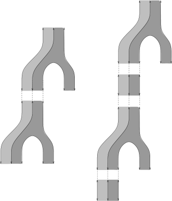
   Figure 2. A quilted surface with strip-like ends and a destabilization of it

2. (Pseudoholomorphic quilts with varying domain) Let $\SS\to\mathcal{R}$ be a smooth family of quilted surfaces with strip-like ends. A pseudoholomorphic quilt for $\SS$ is a datum $(r,\underline{S}_{r}^{\operatorname{ds}},\underline{u})$ where $r\in\mathcal{R}$, $\underline{S}_{r}^{\operatorname{ds}}$ is a destabilization of $\underline{S}_{r}$, $\underline{u}\in C^{\infty}(\underline{S}_{r}^{\operatorname{ds}},\underline{M})$ and $\underline{u}$ satisfies the inhomogeneous pseudoholomorphic map equation on each patch

   (10) $$du_{p}(z)+J_{p}(r,z,u_{p}(z))\circ{\mbox{d}}u_{p}(z)\circ j_{p}(r,z)=Y_{p}(r,z,u_{p}(z))+\\ J_{p}(r,z,u_{p}(z))\circ Y_{p}(r,z,u_{p}(z))\circ j_{p}(r,z),\quad\forall z\in S_{p},\forall p=1,\ldots,k$$

   where $j_{p}(r,z)$ is the complex structure on the quilt $S_{r,p}$ at $z\in S_{r,p}$, and $Y_{p}(r,z)\in\operatorname{Vect}(M_{p})$ is the Hamiltonian vector field associated to the Hamiltonian perturbation $K_{p}(r,z)$.

3. (Isomorphism) Two pseudoholomorphic quilts $(r,\underline{S}_{r}^{\operatorname{ds}},\underline{u}),(r^{\prime},\underline{S}_{r}^{\operatorname{ds},^{\prime}},\underline{u}^{\prime})$ are isomorphic if $r=r^{\prime}$ and there exists an isomorphism of destabilizations $\phi:\underline{S}_{r}^{\operatorname{ds}}\to\underline{S}_{r}^{\operatorname{ds},^{\prime}}$ inducing the identity on $\underline{S}_{r}$ such that $u^{\prime}\circ\phi=u$.

4. (Regular pseudoholomorphic quilts) Associated to any pseudoholomorphic quilt $\underline{u}:\SS^{\operatorname{ds}}\to\underline{M}$ with destabilization $\SS$ is a Fredholm linearized operator for any integer $p>2$

   (11) $$D_{\SS,r,\underline{u}}:T_{r}\mathcal{R}\times\Omega^{0}(\underline{S}^{\operatorname{ds}}_{r},\underline{u}^{*}T\underline{M},\partial\overline{u}^{*}T\underline{L})_{1,p}\to\Omega^{0,1}(\underline{S}_{r}^{\operatorname{ds}},\underline{u}^{*}T\underline{M})_{0,p}\\ (\delta r,\underline{\xi})\mapsto{\frac{1}{2}}(\underline{J}_{\underline{u}}\circ{\mbox{d}}\underline{u}\circ D\underline{j}_{\underline{S}_{r}^{\operatorname{ds}}}(\delta))+D_{\underline{S}_{r}^{\operatorname{ds}},\underline{u}}(\underline{\xi}).$$

   Here $D_{\underline{S}_{r}^{\operatorname{ds}},\underline{u}}(\underline{\xi})$ is the usual linearized Cauchy-Riemann operator of e.g. [22, Chapter 3], acting on the space $\Omega^{0}(\underline{S}^{\operatorname{ds}}_{r},\underline{u}^{*}T\underline{M},\partial\overline{u}^{*}T\underline{L})_{1,p}$ of sections of $\overline{u}^{*}T\underline{M}$ of Sobolev class $W^{1,p}$ with Lagrangian boundary and seam conditions, and $D\underline{j}_{\underline{S}_{r}^{\operatorname{ds}}}(\delta r)$ is the infinitesimal variation of the complex structure on $\underline{S}_{r}^{\operatorname{ds}}$ determined by $\delta r$. A pseudoholomorphic quilt is regular if the associated linearized operator is surjective.

We introduce the following notation for moduli spaces. Denote the moduli space of isomorphism class of pseudoholomorphic quilts with varying domain

$$\mathcal{M}=\{(r,\underline{u}:\underline{S}_{r}^{\operatorname{ds}}\to\underline{M})\}/{\rm isomorphism}.$$

Let $\mathcal{M}(\underline{y}_{\underline{e}},\underline{e}\in\mathcal{E})$ be the subspace of pseudoholomorphic quilts with limits $\underline{y}_{\underline{e}}$ along the ends $\underline{e}\in\mathcal{E}$, and $\mathcal{M}(\underline{y}_{\underline{e}},\underline{e}\in\mathcal{E})_{d}$ the component of formal dimension

$$d=\operatorname{Ind}(D_{\SS,r,\underline{u}})-\dim(\operatorname{aut}(\underline{S}_{r}^{\operatorname{ds}}))$$

where the last term arises from strip components.

The Gromov compactness theorem has a straight-forward generalization to families of pseudoholomorphic quilts, as follows.

Theorem 3.3.

(Gromov compactness for families of quilts) Suppose that $\mathcal{R}$ is a compact stratified space equipped with a family of quilts $\SS\to\mathcal{R}$ with patches labelled by symplectic backgrounds $\underline{M}$ and boundary/seams labelled by Lagrangians $\underline{L}$, and $\mathcal{M}$ is the moduli space of pseudoholomorphic quilts with this data.

1. (Gromov convergence for bounded energy) Any sequence $[\underline{u}_{\nu}:\underline{S}_{r_{\nu}}\to\underline{M}]$ in $\mathcal{M}$ with bounded energy has a Gromov convergent subsequence, that is, a sequence of representatives such that $r_{\nu}$ converges to some $r\in\mathcal{R}$, there exists a destabilization $\underline{S}^{\operatorname{ds}}_{r}$ of $\underline{S}_{r}$, a pseudoholomorphic quilt $\underline{u}:\underline{S}^{\operatorname{ds}}_{r}\to\underline{M}$ and a finite bubbling set $Z\subset\underline{S}^{\operatorname{ds}}_{r}$ such that $\underline{u}_{\nu}$ converges to $\underline{u}$ uniformly in all derivatives on compact subsets of the complement of $Z$:

   $$(G_{\gamma(r_{\nu})})^{*}\lim\underline{u}_{\nu}|C=\underline{u}|C,\quad C\subset\underline{S}-Z\ \text{ compact}$$

   where $G_{\gamma(r_{\nu})}:\underline{S}_{r}^{\operatorname{ds}}\to\overline{S}_{r_{\nu}}$ is the identification of domains given by the gluing parameters in (7).

2. (Convergence in the admissible, low dimension case) If in addition the formal dimension satisfies $d\leq 1$ and all moduli spaces are regular then (sphere and disk) bubbling is ruled out by the monotonicity conditions and the bubbling set is empty (although there still may be bubbling off trajectories on the strip-like ends:)

   $$(d\leq 1)\implies(Z=\emptyset).$$

Proof.

The proof of the first statement is a combination of standard arguments (exponential decay on strip-like ends, energy quantization for sphere and disk bubbles as well as Floer trajectories) and left to the reader. In particular, uniform exponential decay results are also proved in [43, Lemma 3.2.3] for one varying width; the case of several varying widths is similar. For the second statement, suppose a sphere or disk bubble develops for some sequence $\underline{u}_{\nu}:\underline{S}_{\nu}\to\underline{M}$. Any such sphere or disk bubble captures Maslov index at least two, by monotonicity, and so the index of the limiting configuration $\underline{u}:\underline{S}\to\underline{M}$ without the bubbles (obtained by removal of singularities) is at most two less than the indices of the maps $\underline{u}_{\nu}$ in the sequence. But this implies that $\underline{u}$ lies in a component of the moduli space with negative expected dimension, contradicting the regularity assumption. ∎

The Theorem does not quite show that the moduli spaces are compact; for this one needs to show in addition that convergence in the topology whose closed sets are closed under Gromov convergence is the same as Gromov convergence, see [22, 5.6.5].

Next we turn to transversality. The following is a more precise version of Theorem 1.4 of the introduction, that for a sufficiently generic choice of perturbation data the moduli space is a smooth manifold of expected dimension.

Theorem 3.4.

(Existence of a regular extension of perturbation data over the interior) Let $\SS\to\mathcal{R}$ be a family of quilts with patch labels $\underline{M}$ and boundary/seam conditions $\underline{L}$ as in Definition 3.1 so that $\underline{M},\underline{L}$ are in particular monotone. Suppose that a collection of perturbation data $(\underline{J},\underline{K})$ on the restriction of $\SS\to\mathcal{R}$ to the stratified boundary $\partial_{s}\mathcal{R}$ is given such that holomorphic quilted surfaces with strip-like ends of formal dimension at most one are regular. Let $U$ be a sufficiently small open neighborhood of the stratified boundary $\partial_{s}\SS$ with compact complement and let $(\underline{J}_{0},\underline{K}_{0})$ be a pair over $\SS$ agreeing with the complex structures obtained by gluing on $U$. There exists a comeager subset $\mathcal{P}^{\operatorname{{\operatorname{reg}}}}(\SS)$ of the set $\mathcal{P}(\SS)$ of perturbations $(\underline{J},\underline{K})$ agreeing with $(\underline{J}_{0},\underline{K}_{0})$ on slightly smaller open neighborhood $V\subset U$ of $\partial_{s}\SS$ such that every holomorphic quilt with strip-like ends with formal dimension at most one is parametrized regular.

Proof.

First we note regularity of any perturbation system for quilts near the boundary of the moduli space. Indeed for sufficiently small $U\subset\mathcal{R}$ such that $\mathcal{R}\setminus U$ is compact, every pseudoholomorphic quilt $(r,u)$ with $r\in U$ of formal dimension at most one is regular. Indeed, otherwise we would obtain by Gromov convergence a sequence $(r_{\nu},u_{\nu})$ with $r_{\nu}$ converging to a point in the boundary of $\mathcal{R}$. By Gromov compactness, the maps $u_{\nu}$ converge to a map $u:C\to X$ where the domain $C$ is the quilted surface corresponding to $r$ with a collection of disks,, spheres, and Floer trajectories added. After removing these additional disk, spheres one obtains a configuration with lower energy. By the energy-index relation [36, (4)], the index of the resulting configuration would be at most $-1$, and so does not exist by the regularity assumption on the boundary. Hence disk and sphere does not occur and the domain of $u$ is the quilted surface corresponding to $r$, up to the possible addition of strips at the strip-like ends. Since $(r,u)$ is regular by assumption, $(r_{\nu},u_{\nu})$ is also regular by standard arguments involving linearized operators.

A regular extension of the perturbation system over the interior of the family is given by the Sard-Smale theorem. In order to apply it we introduce suitable Banach manifolds of almost complex structures. Let $\mathcal{J}_{U}(\underline{M},\underline{\omega})$ be the set of all smooth $\underline{\omega}$-compatible almost complex structures parametrized by $\SS$, that agree with the original choice on $\SS\setminus\pi^{-1}(V)$ and with the given choices on the images of the strip-like ends. For a sufficiently large integer $l$ let $\mathcal{J}^{l}$ denote the completion of $\mathcal{J}_{U}(\underline{M},\underline{\omega})$ with respect to the $C^{l}$ topology. The tangent space to $\mathcal{J}^{l}$ is the linear space

$$\mathcal{T}_{J}^{l}:=T_{\underline{J}}\mathcal{J}^{l}=\left\{\delta\underline{J}\in C^{l}(\SS\times T\underline{M},T\underline{M})\left|\begin{array}[]{l}\delta\underline{J}\circ\underline{J}+\underline{J}\circ\delta\underline{J}=0\\ \underline{\omega}(\delta\underline{J}(\underline{v}),\underline{w})+\underline{\omega}(v,\delta\underline{J}(w))=0\\ \delta\underline{J}\lvert_{\SS\setminus\pi^{-1}(U)}\equiv 0\end{array}\right.\right\}.$$

For small $\delta\underline{J}$ there is a smooth exponentiation map to $\mathcal{J}^{l}$, given explicitly by $\delta\underline{J}\mapsto\underline{J}\circ\exp(-\underline{J}\circ\delta\underline{J})$. Similarly we introduce suitable Banach spaces of Hamiltonian perturbations. Let $\mathcal{K}^{l}$ denote the completion in the $C^{l}$ norm of the subset $\Omega^{1}_{\SS/\mathcal{R}}(\mathcal{H}(\underline{M});\underline{K})$ of $\Omega^{1}_{\SS/\mathcal{R}}(\mathcal{H}(\underline{M}))$ consisting of 1-forms that equal $\underline{K}$ on the complement of the inverse image of $V$. The tangent space $\mathcal{T}_{K}^{l}:=T_{\underline{K}}\mathcal{K}^{l}$ consists of $\delta\underline{K}\in\Omega^{1}_{\SS/\mathcal{R}}(\mathcal{H}(\underline{M}))$ such that $\delta\underline{K}\lvert_{\SS\setminus V}\equiv 0$. Such elements can be exponentiated to elements of $\mathcal{K}^{l}$ via the map $\underline{K}+\delta\underline{K}$.

Construct a smooth universal space of pseudoholomorphic quilts as follows. Let

$$\mathcal{B}=\{(r,\underline{u})|r\in\mathcal{R},\underline{u}:(\underline{S}_{r},\underline{I}_{r})\to(\underline{M},\underline{L})\}$$

denote the space of pairs $r$ in the parameter space $\mathcal{R}$ and maps $\underline{u}$ from $\underline{S}_{r}$ to $\underline{M}$ of Sobolev class $W^{1,p}$ with seams/boundaries in $\underline{L}$ and

$$\mathcal{E}=\bigcup_{(r,\underline{u})\in\mathcal{B}}\Omega^{0,1}_{\SS/\mathcal{R}}(\underline{u}^{*}T\underline{M})_{0,p}.$$

Here it suffices to consider the case that the domain of $\underline{u}$ is a stable surface, since the strip components are already assumed regular. Since the bundle $\SS\to\mathcal{R}$ is trivializable, $\mathcal{E}$ is a Banach vector bundle of class $C^{l-1}$. The universal moduli space $\mathcal{M}^{\operatorname{univ}}(\underline{y}_{\underline{e}},\underline{e}\in\mathcal{E})\subset\mathcal{B}\times\mathcal{J}^{l}\times\mathcal{K}^{l}$ is a Banach submanifold of class $C^{l-1}$, by a discussion parallel to [22, Lemma 3.2.1]. Indeed, the universal moduli space $\mathcal{M}^{\operatorname{univ}}(\underline{y}_{\underline{e}},\underline{e}\in\mathcal{E})$ is the intersection of the section

$$\overline{\partial}:\mathcal{B}\times\mathcal{J}^{l}\times\mathcal{K}^{l}\to\mathcal{E},\quad(r,\underline{u},\underline{J},\underline{K})\mapsto\overline{\partial}_{\underline{J},\underline{K}}(r,\underline{u})$$

with the zero-section of the bundle $\mathcal{E}\to\mathcal{B}$:

$$\mathcal{M}^{\operatorname{univ}}(\underline{y}_{\underline{e}},\underline{e}\in\mathcal{E}):=\overline{\partial}^{-1}(0).$$

To show that the universal moduli space is a Banach manifold, it suffices to show that the linearized operator

(12) $$D_{\SS,r,\underline{u},J,K}:T_{(r,\underline{u})}\mathcal{B}\times\mathcal{T}_{J}^{l}\times\mathcal{T}_{K}^{l}\longrightarrow\mathcal{E}_{\SS,r,\underline{u}}\\ (\delta r,\underline{\xi},\delta\underline{J},\delta\underline{K})\mapsto(\delta\underline{Y})^{0,1}+\underline{j}_{\underline{S}_{r}}\circ\frac{1}{2}(d\underline{u}-\underline{Y})\circ\delta\underline{J}+D_{\SS,r,\underline{u}}(\delta r,\underline{\xi})$$

is surjective at all $(r,\underline{u},\underline{J},\underline{K})$ for which $\overline{\partial}_{(\underline{J},\underline{K})}(r,\underline{u})=0$. Since the last operator in (12) is Fredholm, the image of $D_{\SS,r,\underline{u},\underline{J},\underline{K}}$ is closed.

We prove that the linearized operator cutting out the universal moduli space is surjective. Suppose that the cokernel is not zero. By the Hahn-Banach theorem, there exists a linear functional

$$\eta\in(\mathcal{E}_{\SS,r,\underline{u}})^{*}=L^{q}(\underline{S}_{r},(\Omega_{\underline{S}_{r}}^{0,1}\otimes\underline{u}^{*}T\underline{M})),\quad 1/p+1/q=1$$

that is non-zero and that vanishes on the image of the linearized operator. In particular $\eta$ vanishes on the image of $D_{\underline{S}_{r},\underline{u}}$, i.e.

$$\int_{\underline{S}_{r}}\langle D_{\underline{S}_{r},\underline{u}}(\underline{\xi}),\eta\rangle=0=\int_{\underline{S}_{r}}\langle\underline{\xi},D_{\underline{S}_{r},\underline{u}}^{*}(\eta)\rangle$$

for all $\underline{\xi}\in W^{1,p}(\underline{S}_{r},\underline{u}^{*}T\underline{M})$. This argument implies $D_{\underline{S}_{r},\underline{u}}^{*}(\eta)=0$, and elliptic regularity ensures that $\eta$ is of class $C^{l}$ at least in the interiors of the patches of the quilt $\underline{S}_{r}$. To prove that $\eta$ is zero, it suffices to show that it vanishes on an open subset of each patch of the quilt $\underline{S}_{r}$, since by unique continuation for solutions of $D_{\underline{S}_{r},\underline{u}}^{*}\eta=0$ it follows that it vanishes on all of $\underline{S}_{r}$. We may assume that the complement of the images of the strip-like ends contains such an open subset. Considering the image of $(0,0,0,\delta\underline{K})$ shows that

$$\int_{\underline{S}_{r}}\langle(\delta\underline{Y})^{0,1},\eta\rangle=0$$

for all $\delta\underline{Y}$, where $\delta\underline{Y}$ is the Hamiltonian vector field associated to $\delta\underline{K}$. But now, for each $z$ in the complement of the inverse image of $U$ and the complement of the images of the strip-like ends, there exists a sequence of functions $\delta\underline{K}_{n}$ in $\mathcal{T}_{\underline{K}}^{l}$ that are supported on successively smaller neighborhoods of $z$ and such that $(\delta\underline{Y}_{n})^{0,1}$ converges to the delta function $\delta_{z}\otimes\eta(z)$. It follows that there exists a limit

$$|\eta(z)|^{2}=\lim_{n\to\infty}\int_{\underline{S}_{r}}\langle(\delta\underline{Y}_{n})^{0,1},\eta\rangle=0.$$

So $\eta(z)=0$ on an open subset of each patch of the quilt. By unique continuation it must vanish everywhere. Thus, $\eta=0$, which is a contradiction. Hence the linearized operator is surjective, so by the implicit function theorem for $C^{l-1}$ maps of Banach spaces, $\mathcal{M}^{\operatorname{univ}}(\underline{y}_{\underline{e}},\underline{e}\in\mathcal{E})$ is also a Banach manifold of class $C^{l-1}$. One can now consider the projection

$$\Pi:\mathcal{M}^{\operatorname{univ}}(\underline{y}_{\underline{e}},e\in\mathcal{E})_{d}\to\mathcal{J}^{l}\times\mathcal{K}^{l},\ \ (r,\underline{u},\underline{J},\underline{K})\mapsto(\underline{J},\underline{K})$$

on the subset $\mathcal{M}^{\operatorname{univ}}(\underline{y}_{\underline{e}},\underline{e}\in\mathcal{E})_{d}$ of parametrized index $d$, which is a Fredholm map between Banach manifolds of index $d$. By the Sard-Smale theorem, for $l>\max(d,0)$ the subset of regular values

$$\mathcal{P}_{{\operatorname{reg}}}^{l}=\{(\underline{J},\underline{K})\in\mathcal{J}^{l}\times\mathcal{K}^{l}\ |\ \operatorname{coker}(D_{r,\underline{u},\underline{J},\underline{K}}\Pi)=0,\ \ \forall(r,\underline{u},\underline{J},\underline{K})\in\mathcal{M}^{\operatorname{univ}}(\underline{y}_{\underline{e}})\}$$

is comeager, hence dense. Now the regular values of the projection correspond precisely to regular perturbation data for the moduli spaces $\mathcal{M}(\underline{y}_{\underline{e}},\underline{e}\in\mathcal{E})$, thus the subset of regular $C^{l}$-smooth perturbation data comeager in $\mathcal{J}^{l}\times\mathcal{K}^{l}$.

The final step is to pass from $C^{l}$-smooth regular perturbation data, to $C^{\infty}$ regular perturbation data. This is a standard argument due to Taubes, see Floer-Hofer-Salamon [8] and McDuff-Salamon [22] for its use in pseudoholomorphic curves, which we explain in the unquilted case for simplicity. Let us write

$$\mathcal{J}:=\bigcap_{l\geq 0}\mathcal{J}^{l},\quad\mathcal{K}:=\bigcap_{l\geq 0}\mathcal{K}^{l},\quad\mathcal{P}:=\mathcal{J}\times\mathcal{K}$$

with the $C^{\infty}$ topology on each factor. Let $C>0$ be a constant such that any pseudoholomorphic quilt has exponential decay satisfying $|{\mbox{d}}u(s,t)|<\exp(-Cs)$ for all $(s,t)$ coordinates on each end $\underline{e}\in\mathcal{E}$, see [37, Theorem 5.2.4]. Let $\psi:S\to\mathbb{R}$ be a positive function given by $\psi(s,t)=s$ on each end, for each surface $S_{r},r\in\mathcal{R}$. For $k>0$, let $\mathcal{P}_{{\operatorname{reg}},k}\subset\mathcal{P}$ consist of the perturbation data for which the associated linearized operators $D_{\SS,\underline{u}}$ are surjective for all $\underline{u}\in\mathcal{M}(\underline{y}_{\underline{e}},\underline{e}\in\mathcal{E})$ satisfying

(13) $$\operatorname{ind}D_{\SS,\underline{u}}\in\{0,1\},\ \ \|{\mbox{d}}\underline{u}\exp(C\psi)\|_{L^{\infty}}\leq k.$$

The index restrictions above suffice since we only consider moduli spaces of expected dimension 0 and 1. We will show that the set

$$\mathcal{P}_{{\operatorname{reg}}}:=\bigcap_{k>0}\mathcal{P}_{{\operatorname{reg}},k}$$

is comeager in $\mathcal{P}$, by showing that each of the sets $\mathcal{P}_{{\operatorname{reg}},k}$ is open and dense in $\mathcal{P}$ with respect to the $C^{\infty}$ topology.

To show that $\mathcal{P}_{{\operatorname{reg}},k}$ is open, consider a sequence $\{(\underline{J}_{\nu},\underline{K}_{\nu})\}_{\nu=1}^{\infty}$ in the complement of $\mathcal{P}_{{\operatorname{reg}},k}$, converging in the $C^{\infty}$ topology to a pair $(\underline{J}_{\infty},\underline{K}_{\infty})$. We claim that $(\underline{J}_{\infty},\underline{K}_{\infty})\notin\mathcal{P}_{{\operatorname{reg}},k}$. By assumption, there exists a sequence $\underline{u}_{\nu}$ such that

$$\overline{\partial}_{\underline{J}_{\nu},\underline{K}_{\nu}}\underline{u}_{\nu}=0\quad\operatorname{ind}D_{\SS,\underline{u}}\in\{0,1\},\quad\|\underline{u}_{\nu}\|_{L^{\infty}}\leq k.$$

We may take the elements of the sequence to have the same index. The uniform bound on the derivative $\|{\mbox{d}}\underline{u}_{\nu}\exp(C\psi)\|_{L^{\infty}}\leq k$ implies that $\underline{u}_{\nu}$ converges to a pseudoholomorphic quilt. Since surjectivity of Fredholm operators is an open condition, $D_{\SS,\underline{u}_{\nu}}$ must be surjective for sufficiently large $\nu$. This argument proves that $\mathcal{P}_{{\operatorname{reg}},k}$ is open in $\mathcal{P}$ for each $k>0$.

To show that $\mathcal{P}_{{\operatorname{reg}},k}$ is dense, note that we can write $\mathcal{P}_{{\operatorname{reg}},k}=\mathcal{P}^{l}_{{\operatorname{reg}},k}\cap\mathcal{P}$, where the definition of $\mathcal{P}^{l}_{{\operatorname{reg}},k}$ is the same as the definition for $\mathcal{P}_{{\operatorname{reg}},k}$, but as a subset of $\mathcal{P}^{l}$. The argument given above to prove that $\mathcal{P}_{{\operatorname{reg}},k}$ is open in $\mathcal{P}$ with respect to the $C^{\infty}$ topology can be repeated to show that for all sufficiently large $l$ the subset $\mathcal{P}_{{\operatorname{reg}},k}^{l}$ is open in $\mathcal{P}^{l}$ with respect to the $C^{l}$ topology. The set $\mathcal{P}_{{\operatorname{reg}}}^{l}$ is dense $\mathcal{P}^{l}$, and since $\mathcal{P}_{{\operatorname{reg}},k}^{l}\supset\mathcal{P}_{{\operatorname{reg}}}^{l}$, this implies that $\mathcal{P}_{{\operatorname{reg}},k}^{l}$ is dense in $\mathcal{P}^{l}$. So fix $(\underline{J},\underline{K})\in\mathcal{P}$. We find a sequence $(\underline{J}_{\nu},\underline{K}_{\nu})\in\mathcal{P}_{{\operatorname{reg}},k}$ that converges to $(\underline{J},\underline{K})$ in the $C^{\infty}$ topology. Consider a sequence

$$(\underline{J}_{l},\underline{K}_{l})\in\mathcal{P}_{{\operatorname{reg}},k}^{l},\quad\|\underline{J}_{l}-\underline{J}\|_{C^{l}}+\|\underline{K}_{l}-\underline{K}\|_{C^{l}}\leq 2^{-l}.$$

Such a sequence exists because $\mathcal{P}_{{\operatorname{reg}},k}^{l}$ is dense in $\mathcal{P}^{l}$ for each $l$, and $(\underline{J},\underline{K})\in\mathcal{P}\subset\mathcal{P}^{l}$. Now, by assumption $\mathcal{P}_{{\operatorname{reg}},k}^{l}$ is open in $\mathcal{P}^{l}$, and so for each $(\underline{J}_{l},\underline{K}_{l})\in\mathcal{P}^{l}$ there exists an $\epsilon_{l}>0$ such that

$$\|\underline{J}-\underline{J}_{l}\|_{C^{l}}+\|\underline{K}-\underline{K}_{l}\|_{C^{l}}<\epsilon_{l}\implies(\underline{J},\underline{K})\in\mathcal{P}_{{\operatorname{reg}},k}^{l}$$

for all $(\underline{J},\underline{K})\in\mathcal{P}^{l}$. Finally, $\mathcal{P}$ is dense in $\mathcal{P}^{l}$ for each $l$ (i.e. $C^{\infty}$ functions are dense in the space of $C^{l}$ functions). Therefore, for each $l$ we may find an element $(\tilde{\underline{J}}_{l},\tilde{\underline{K}}_{l})\in\mathcal{P}$ such that

$$\|\tilde{\underline{J}}_{l}-\underline{J}_{l}\|_{C^{l}}+\|\tilde{\underline{K}}_{l}-\underline{K}_{l}\|_{C^{l}}<\min\{\epsilon_{l},2^{-l}\}.$$

Thus, every term in the sequence $(\tilde{\underline{J}}_{l},\tilde{\underline{K}}_{l})$ is in $\mathcal{P}\cap\mathcal{P}_{{\operatorname{reg}},k}^{l}=\mathcal{P}_{{\operatorname{reg}},k}$, and it converges in all $C^{l}$ norms, hence in the $C^{\infty}$ topology, to the pair $(\underline{J},\underline{K})$. Thus, $\mathcal{P}_{{\operatorname{reg}}}=\underset{k>0}{\cap}\mathcal{P}_{{\operatorname{reg}},k}$ is a countable intersection of open, dense sets in $\mathcal{P}$ as claimed. ∎

Remark 3.5.

1. (Zero and one-dimensional components of the moduli spaces) For $d=0$, the moduli space $\mathcal{M}_{\SS}(\underline{y}_{\underline{e}},\underline{e}\in\mathcal{E})_{d}$ lies entirely over the highest dimensional strata of $\mathcal{R}$. On the other hand for $d=1$ the intersection with the highest dimensional strata is one-dimensional, while the intersection with the codimension one strata is a discrete set of points.

2. (Comparison with Seidel) Seidel’s book [29] uses perturbations that are supported arbitrarily close to the boundary. The advantage of these is that one can make the higher-dimensional moduli spaces regular as well. However, only the zero and one-dimensional moduli spaces are needed here.

Remark 3.6.

(Orientations for families of pseudoholomorphic quilts) To define family quilt invariants over the integers we require that the moduli spaces are oriented. Orientations on the moduli spaces may be constructed as follows [41]. At any element $(r,\underline{u})\in\mathcal{M}_{\SS}(\underline{y}_{\underline{e}},\underline{e}\in\mathcal{E})$ the tangent space to the moduli space of pseudoholomorphic quilts is the kernel of the linearized operator (11). The operator $D_{\underline{u}}$ is canonically homotopic to the operator $0\oplus D_{\underline{u},r}$ (the latter is the operator for the trivial family $\{r\}$, that is, the unparametrized linearized operator) via a path of Fredholm operators. This induces an isomorphism

(14) $$\operatorname{det}(T_{(r,\underline{u})}\mathcal{M}(\underline{y}_{\underline{e}},\underline{e}\in\mathcal{E}))\to\operatorname{det}(T_{r}\mathcal{R})\otimes\operatorname{det}(D_{\underline{u}}).$$

First one deforms the seam conditions $\underline{u}^{*}T\underline{L}$ to condition of split type, that is for each seam $I$ adjacent to patches $S_{p_{-}},S_{p_{+}}$ deform the map $I\to\operatorname{Lag}(M_{p_{-}}\times M_{p_{+}})$ defined by $u,\underline{L}$ to a map $I\to\operatorname{Lag}(M_{p_{-}})\times\operatorname{Lag}(M_{p_{+}})$. This deformation identifies the corresponding determinant lines and reduces the claim to the case of an unquilted pseudoholomorphic map $u:\underline{S}_{r}\to M$ with boundary condition $L$. The determinant line $\operatorname{det}(D_{u})$ is oriented by “bubbling off one-pointed disks”, see [11, Theorem 44.1] or [41, Equation (36)]. The orientation at $u$ is determined by an isomorphism

(15) $$\operatorname{det}(D_{{u}})\cong\mathcal{D}^{+}_{{x}_{0}}\mathcal{D}^{-}_{x_{1}}\ldots\mathcal{D}^{-}_{x_{d}}$$

where $\mathcal{D}^{+}_{x_{j}}$ are determinant lines associated with one-marked disks with marking ${x}_{j}$, $\mathcal{D}^{-}_{x_{j}}$ is the tensor product of the determinant line for the once-marked disk with $\operatorname{det}(T_{x_{j}}L)$ and the orientations on $\mathcal{D}^{\pm}_{x_{j}}$ are chosen so that there is a canonical isomorphism $\mathcal{D}^{-}_{x_{j}}\otimes\mathcal{D}^{+}_{x_{j}}\to\mathbb{R}.$ The isomorphism (15) is determined by degenerating surface with strip-like ends to a nodal surface with each end replaced by a disk with one end attached to the rest of the surface by a node. The boundary condition on these disks is given by a chosen path of Lagrangian subspaces in the tangent space at the end. Furthermore, the Lagrangian boundary condition is deformed to a constant boundary condition using the relative spin structure. These choices are analogous to choice of orientations on the tangent spaces to the stable manifolds in Morse theory, on which the orientations of the moduli spaces of Morse trajectories depend.

The master equation for family quilt invariants is a consequence of the following description of the boundary of the one-dimensional moduli spaces of quilts:

Theorem 3.7.

(Description of the boundary of one-dimensional moduli spaces of pseudoholomorphic quilts) Suppose that $\SS\to\mathcal{R}$ is a family of quilted surfaces over a compact stratified space $\mathcal{R}$ with a single open stratum denoted $\SS_{0}\to\mathcal{R}_{0}$ labelled with monotone symplectic data $\underline{M},\underline{L}$, and $\underline{J},\underline{K}$ are a regular set of perturbation data. Then for any limits $\underline{y}_{\underline{e}},\underline{e}\in\mathcal{E}$

1. (Zero-dimensional component) the zero-dimensional component $\mathcal{M}_{\SS}(\underline{y}_{\underline{e}},\underline{e}\in\mathcal{E})_{0}$ of the moduli space of pseudoholomorphic quilts for $\SS$ is a finite set of points and

2. (One-dimensional component) the one-dimensional component $\mathcal{M}_{\SS_{0}}(\underline{y}_{\underline{e}},\underline{e}\in\mathcal{E})_{1}$ has a compactification as a one-manifold with boundary

   (16) $$\partial\mathcal{M}_{\SS}(\underline{y}_{\underline{e}},\underline{e}\in\mathcal{E})_{1}=\mathcal{M}_{\partial\SS}(\underline{y}_{\underline{e}},\underline{e}\in\mathcal{E})_{1}\\ \cup\bigcup_{{\underline{f}}\in\mathcal{E}}\mathcal{M}(y_{\underline{f}},y_{\underline{f}}^{\prime})_{0}\times\mathcal{M}_{\SS}(\underline{y}_{\underline{e}},\underline{e}\in\mathcal{E};\underline{y}_{\underline{f}}\mapsto\underline{y}_{\underline{f}}^{\prime})_{0}$$

   with sign of inclusion given by $+1$ for the first factor and $\pm 1$ for the second factor, depending on whether $\underline{y}_{\underline{f}}$ is an incoming or outgoing end. Here $\mathcal{M}_{\SS}(\underline{y}_{\underline{e}},\underline{e}\in\mathcal{E};\underline{y}_{\underline{f}}\mapsto\underline{y}_{\underline{f}}^{\prime})_{1}$ denotes $\mathcal{M}_{\SS}(\underline{y}_{\underline{e}},\underline{e}\in\mathcal{E})$ with the end label $\underline{y}_{\underline{f}}$ replaced by $\underline{y}_{\underline{f}}^{\prime})_{1}$ while $\mathcal{M}(y_{\underline{f}},y_{\underline{f}}^{\prime})_{0}$ denotes the space of Floer trajectories from $y_{\underline{f}}$ to $y_{\underline{f}}^{\prime}$ of formal dimension $0$.

Proof.

The gluing theorem is proved in the same way as for Ma’u [21], who considered the gluing along strip-like ends that arise in the definition of the generalized Fukaya category. Compactness is Theorem 3.3. The claim on orientations is proved in [41]. ∎

Finally we use the moduli spaces of quilts to construct chain-level invariants. Let $\mathcal{R}$ be a stratified space labelled by quilt data $\underline{M},\underline{L}$ as in Theorem 1.4, and $\SS\to\mathcal{R}$ a family of quilted surfaces with strip-like ends constructed in Section 2.

Definition 3.8.

(Family quilt invariants) Given a regular pair $(\underline{J},\underline{K})$ as in Theorem 1.4 we define a (cochain level) family quilt invariant

$$\Phi_{\SS}:\bigotimes_{\underline{e}\in\mathcal{E}_{-}(\SS)}CF(\underline{L}_{\underline{e}})\to\bigotimes_{\underline{e}\in\mathcal{E}_{+}(\SS)}CF(\underline{L}_{\underline{e}})$$

by

$$\Phi_{\SS}\biggl{(}\bigotimes_{\underline{e}\in\mathcal{E}_{-}}\langle{\underline{x}^{-}_{\underline{e}}}\rangle\biggr{)}:=\sum_{\underline{u}\in\mathcal{M}_{\SS}(\langle{\underline{x}_{\underline{e}}}\rangle_{\underline{e}\in\mathcal{E}_{-}},\langle{\underline{x}_{\underline{e}}}\rangle_{\underline{e}\in\mathcal{E}_{+}})_{0}}\sigma(u)\bigotimes_{\underline{e}\in\mathcal{E}_{+}}\langle{\underline{x}^{+}_{\underline{e}}}\rangle,$$

where

$$\sigma:\mathcal{M}_{\SS}(x_{\underline{e}},\underline{e}\in\mathcal{E})_{0}\to\{-1,+1\}$$

is defined by comparing the orientation to the canonical orientation of a point.

Theorem 1.5 follows from Theorem 3.7 and the following discussion of orientations. In particular, if $\mathcal{R}$ has no codimension one strata, then $\Phi_{\SS}$ is a cochain map. The case that $\mathcal{R}$ is a point was considered in [36].

4. The Fukaya category of generalized Lagrangian branes

In the remainder of the paper we apply the results of the first two sections to construct $A_{\infty}$ categories, $A_{\infty}$ functors, $A_{\infty}$ pre-natural transformations and $A_{\infty}$ homotopies and prove Theorems 1.1 and 1.2 from the introduction. The Fukaya category of a symplectic manifold, when it exists, is an $A_{\infty}$ category whose objects are Lagrangian submanifolds with certain additional data, and morphism spaces are Floer cochain spaces. In [42] we explained that in order to obtain good functoriality properties one should allow certain more general objects, which we termed generalized Lagrangian branes, comprised of sequences of Lagrangian correspondences. The necessary analysis for defining Fukaya categories with these generalized objects for compact monotone symplectic manifolds was developed by the first author in [21], and extends the constructions of Fukaya [10] and Seidel [29] to include generalized Lagrangian branes as introduced in [42].

4.1. Quilted Floer cochain groups

In this section we review the construction of Floer cochain groups for certain symplectic manifolds with additional structure. The cochain groups are the morphism spaces in the version of the Fukaya category on which our functors are defined. We begin by stating the technical hypotheses under which our Floer cochain complexes are well-defined.

Definition 4.1.

(Symplectic backgrounds) Fix a monotonicity constant $\tau\geq 0$ and an even integer $N>0$. A symplectic background is a tuple $(M,\omega,b,\operatorname{Lag}^{N}(M))$ as follows.

1. (Bounded geometry) $M$ is a smooth manifold, which is compact if $\tau>0$.

2. (Monotonicity) $\omega$ is a symplectic form on $M$ which is monotone, i.e. $[\omega]=\tau c_{1}(TM)$ and if $\tau=0$ then $M$ satisfies “bounded geometry” assumptions as in e.g. [29].

3. (Background class) $b\in H^{2}(M,\mathbb{Z}_{2})$ is a background class, which will be used for the construction of orientations.

4. (Maslov cover) $\operatorname{Lag}^{N}(M)\to\operatorname{Lag}(M)$ is an $N$-fold Maslov cover in the sense of [28], [37] such that the induced $2$-fold Maslov covering $\operatorname{Lag}^{2}(M)$ is the oriented double cover.

We often refer to a symplectic background $(M,\omega,b,\operatorname{Lag}^{N}(M))$ as $M$.

Example 4.2.

(Point background) The point $M=\{\operatorname{pt}\}$ can be viewed as a canonical $\tau$-monotone, $N$-graded symplectic background $(\{\operatorname{pt}\},\omega=0,b=0,\operatorname{Lag}^{N}(\operatorname{pt}))$, which we denote by $\operatorname{pt}$.

Next introduce Lagrangian branes, which will be the objects of the Fukaya categories we consider. Let $M$ be a symplectic background.

Definition 4.3.

(Admissible Lagrangians)

1. A Lagrangian submanifold $L\subset M$ is admissible if

   1. $L$ is compact and oriented;

   2. $L$ is monotone, that is, for $u:(D,\partial D)\to(M,L)$ the symplectic action $A(u)$ and index $I(u)$ are related by

      $$2A(u)=\tau I(u)\quad\forall u:(D,\partial D)\to(M,L),$$

      where $\tau$ is the monotonicity constant for $M$;

   3. $L$ has minimal Maslov number at least $3$, or minimal Maslov number $2$ and disk invariant $\Phi_{L}=0$ in the sense of [25] (that is, the signed count of Maslov index $2$ disks with boundary on $L$); and

   4. the image of $\pi_{1}(L)$ in $\pi_{1}(M)$ is torsion, for any choice of base point.

2. An admissible grading of an oriented Lagrangian submanifold $L\subset M$ is a lift

   $$\sigma_{L}^{N}:L\to\operatorname{Lag}^{N}(M)$$

   of the canonical section $L\to\operatorname{Lag}(M)$ such that the induced lift $\sigma_{L}^{2}$ equals to the lift induced by the orientation. See [37] for details.

3. A relative spin structure on an admissible Lagrangian submanifold $L\subset M$ with respect to the background class

   $$b\in H^{2}(M,\mathbb{Z}_{2})$$

   is [11],[41] a lift of the class of $TL$ defined in the first relative Čech cohomology group for the inclusion $i:L\to M$ with values in $\operatorname{SO}(\dim(L))$ to first relative Čech cohomology with values in $\operatorname{Spin}(\dim(L)))$, with associated class $b$.

Recall that a Lagrangian correspondence is a Lagrangian submanifold of a product of symplectic manifold with the symplectic form on the first factor reversed. Given symplectic manifolds $M_{0}$ and $M_{1}$ and a Lagrangian correspondence $L_{01}\subset M_{0}^{-}\times M_{1}$, the transpose of $L_{01}$ is the generalized Lagrangian correspondence $L_{01}^{T}$ from $M_{1}$ to $M_{0}$ obtained by applying the anti-symplectomorphism $M_{0}^{-}\times M_{1}\to M_{1}^{-}\times M_{0},\ (m_{0},m_{1})\mapsto(m_{1},m_{0})$ to $L_{01}$.

Definition 4.4.

(Generalized Lagrangian branes) Let ${M_{s}}:=(M_{s},\omega_{s},b_{s},\operatorname{Lag}^{N}(M_{s}))$ and ${M_{t}}:=(M_{t},\omega_{t},b_{t},\operatorname{Lag}^{N}(M_{t}))$ be two symplectic backgrounds. A generalized Lagrangian brane from ${M_{s}}$ to ${M_{t}}$ is a tuple $\underline{L}=(L_{(j-1)j})_{j=1,\ldots,r}$ of length $r\geq 0$ of Lagrangian correspondences equipped with gradings, relative spin structures, and widths as follows.

1. (Sequence of backgrounds) $(N_{i},\omega_{i},b_{i},\operatorname{Lag}^{N}(N_{i}))_{i=0,\ldots,r}$ is a sequence of symplectic backgrounds such that $N_{0}=M_{s}$ and $N_{r}=M_{t}$ as symplectic backgrounds;

2. (Sequence of correspondences) $L_{(j-1)j}\subset N_{j-1}^{-}\times N_{j}$ is an admissible Lagrangian submanifold for each $j=1,\ldots,r$ with respect to $-\pi_{j-1}^{*}\omega_{j-1}+\pi_{j}^{*}\omega_{j}$, where $\pi_{j-1},\pi_{j}$ are the projections to the factors of $N_{j-1}^{-}\times N_{j}$;

3. (Gradings) a grading on $\underline{L}$, by which we mean a collection of gradings

   $$\sigma_{L_{(j-1)j}}^{N}:L_{(j-1)j}\to\operatorname{Lag}^{N}(N_{j-1}^{-}\times N_{j})$$

   for $j=1,\ldots,r$ with respect to the Maslov cover induced by the product of covers of $N_{j-1}$ and $N_{j}$.

4. (Relative spin structures) a relative spin structure on $\underline{L}$ is a collection of relative spin structures on $L_{(j-1)j}$ for $j=1,\ldots,r$ with background classes $-\pi_{j-1}^{*}b_{j-1}+\pi_{j}^{*}b_{j}$;

5. (Widths) a collection of widths $\underline{\delta}=(\delta_{j}>0)_{j=1,\ldots,r-1}$.

Let ${M}:=(M,\omega,b,\operatorname{Lag}^{N}(M))$ be a symplectic background. Then a generalized Lagrangian brane in ${M}$ is a generalized Lagrangian brane from $\operatorname{pt}$ to $M$.

Next we define brane structures on Lagrangian correspondences. Given symplectic backgrounds $M_{s},M_{t},M_{u}$ with the same monotonicity constant, admissible generalized Lagrangian correspondence branes $\underline{L}^{+},\underline{L}^{-}$ from $M_{s}$ to $M_{t}$ resp. $M_{t}$ to $M_{u}$ with the same background class in $M_{t}$ and width $\epsilon>0$ we can concatenate them to obtain a generalized Lagrangian correspondence $\underline{L}^{+}\includegraphics[height=5.05942pt]{sharp.eps}_{\epsilon}\underline{L}^{-}$ from $M_{s}$ to $M_{u}$. More precisely, we define $\underline{L}:=\underline{L}^{+}\includegraphics[height=5.05942pt]{sharp.eps}_{\epsilon}(\underline{L}^{-})^{T}$ to be the generalized Lagrangian correspondence with gradings and relative spin structures, given as follows:

1. symplectic backgrounds with the same monotonicity constant indexed up to $r:=r^{+}+r^{-}$

   $$(N_{0},\ldots,N_{r}):=\bigl{(}M_{s}=N^{+}_{0},\ldots,N^{+}_{r^{+}}=M_{t}=N^{-}_{r^{-}},\ldots,N^{-}_{0}=M_{u}\bigr{)};$$

2. the admissible Lagrangian submanifolds

   (17) $$(L_{01},\ldots,L_{(r^{+}+r^{-}-1)(r^{+}+r^{-})}):=\bigl{(}L^{+}_{01},\ldots,L^{+}_{(r^{+}-1)r^{+}},L^{-}_{01},\ldots,L^{-}_{(r^{-}-1)r^{-}}\bigr{)};$$

3. the relative spin structures on $L^{+}_{(j-1)j}$ for $j=1,\ldots,r^{+}$ and the relative spin structures on $L_{(j-1)j}^{-}$ induced from those on $L_{(j-1)j}^{-}$ for $j=1,\ldots,r^{-}$;

4. the widths are those of $\underline{L}^{+},\underline{L}^{-}$ together with $\epsilon$.

In particular given symplectic backgrounds $M_{s},M_{t}$ with the same monotonicity constant, admissible generalized Lagrangian correspondence branes $\underline{L}^{+},\underline{L}^{-}$ from $M_{s}$ to $M_{t}$, and width $\epsilon>0$ we can transpose one and then concatenate them to obtain a cyclic Lagrangian correspondence $\underline{L}^{+}\includegraphics[height=5.05942pt]{sharp.eps}_{\epsilon}(\underline{L}^{-})^{T}$. Here the gradings $\sigma_{L^{-}_{(j-1)j}}^{N}$ of $L^{-}_{(j-1)j}$ for $j=1,\ldots,r^{+}$ inducing gradings of $(L_{(j-1)j}^{-})^{T}$ for $j=1,\ldots,r^{-}$ and similarly for the relative spin structures. The resulting sequence can be visualized as

$$\begin{diagram}$$

The Floer cohomology of a cyclic generalized Lagrangian correspondence is defined as follows. Choose regular Hamiltonian perturbations

$$\underline{H}\in\oplus_{j=0}^{r}C^{\infty}([0,\delta_{j}]\times N_{j}),$$

and almost complex structures

$$\underline{J}\in\oplus_{j=0}^{r}C^{\infty}([0,\delta_{j}],\mathcal{J}(N_{j},\omega_{j}))$$

as in [38]. The generators of the quilted Floer cochain complex of a generalized Lagrangian brane $\underline{L}$ are the perturbed intersection points

$$\mathcal{I}(\underline{L}):=\left\{\underline{x}=\bigl{(}x_{j}:[0,\delta_{j}]\to N_{j}\bigr{)}_{j=0,\ldots,r}\,\left|\begin{aligned} \dot{x}_{j}(t)=Y_{j}(t,x_{j}(t)),\\ (x_{j}(\delta_{j}),x_{j+1}(0))\in L_{j(j+1)}\end{aligned}\quad\forall j\right.\right\}.$$

Here $Y_{j}$ is the Hamiltonian vector field corresponding to $H_{j}$. The gradings on $\underline{L}$ induce a grading $|\underline{x}|\in\mathbb{Z}_{N}$ for $\underline{x}\in\mathcal{I}(\underline{L})$, and hence induce a $\mathbb{Z}_{N}$-grading on the space of quilted Floer cochains

$$CF(\underline{L}):=\bigoplus_{\underline{x}\in\mathcal{I}(\underline{L})}\mathbb{Z}\langle{\underline{x}}\rangle=\bigoplus_{k\in\mathbb{Z}_{N}}CF^{k}(\underline{L}),\qquad CF^{k}(\underline{L}):=\bigoplus_{|\underline{x}|=k}\mathbb{Z}\langle{\underline{x}}\rangle.$$

The Floer coboundary operator is defined by counts of the moduli spaces of quilted pseudoholomorphic strips,

$$\partial:\ CF^{\bullet}(\underline{L})\to CF^{\bullet+1}(\underline{L}),\quad\langle{\underline{x}_{-}}\rangle\mapsto\sum_{\underline{x}_{+}\in\mathcal{I}(\underline{L})}\Bigl{(}\sum_{\underline{u}\in\mathcal{M}(\underline{x}_{-},\underline{x}_{+})_{0}}\epsilon(\underline{u})\Bigr{)}\langle{\underline{x}_{+}}\rangle,$$

where the signs

(18) $$\epsilon:\mathcal{M}(\underline{x}_{-},\underline{x}_{+})_{0}\to\{\pm 1\}$$

are given by the orientation of the moduli space

$$\mathcal{M}(\underline{x}_{-},\underline{x}_{+})_{0}:=\bigl{\{}\underline{u}=\bigl{(}u_{j}:\mathbb{R}\times[0,\delta_{j}]\to N_{j}\bigr{)}_{j=0,\ldots,r}\,\big{|}\,\eqref{Jjhol}-\eqref{ulim2},\operatorname{Ind}(D_{\underline{u}})=1\bigr{\}}/\mathbb{R}$$

of tuples of pseudoholomorphic maps

(19) $$\overline{\partial}_{J_{j},H_{j}}u_{j}=\partial_{s}u_{j}+J_{j}\bigl{(}\partial_{t}u_{j}-Y_{j}(u_{j})\bigr{)}=0\qquad\forall j=0,\ldots r,$$

satisfying the seam conditions

(20) $$(u_{j}({s},\delta_{j}),u_{j+1}({s},0))\in L_{j(j+1)}\qquad\forall j=0,\ldots r,\ s\in\mathbb{R},$$

with finite energy

(21) $$\sum_{j=0}^{r}\int_{\mathbb{R}\times[0,\delta_{j}]}u_{j}^{*}\omega_{j}+{\rm d}(H_{j}(u_{j}){\rm d}t)<\infty,$$

and prescribed limits

(22) $$\qquad\lim_{s\to\pm\infty}u_{j}(s,\cdot)=x^{\pm}_{j}\quad\forall j=0,\ldots,r.$$

The Floer coboundary operator is the first in a sequence of operators associated to pseudoholomorphic quilts with varying domain. In [37] we showed that $\partial^{2}=0$, and hence the quilted Floer cohomology

$$HF^{\bullet}(\underline{L})=H^{\bullet}(CF(\underline{L},\partial))$$

is well defined. Here we work on chain level, and in case $M_{s}=\operatorname{pt}$ interpret $\partial=:\mu^{1}$ as the first of the $A_{\infty}$ composition maps on ${\operatorname{Fuk}^{\includegraphics[height=5.05942pt]{sharp.eps}}}(M)$,

$$\mu^{1}:CF^{\bullet}(\underline{L}^{+},\underline{L}^{-})\to CF^{\bullet+1}(\underline{L}^{+},\underline{L}^{-}).$$

The objects in the extended Fukaya category are generalized Lagrangian branes. The morphism spaces in the extended Fukaya category are the quilted Floer chain complex associated to the cyclic generalized Lagrangian correspondence $\underline{L}$ of length $r=r^{+}+r^{-}$ shifted in degree

$$\operatorname{Hom}(\underline{L}^{+},\underline{L}^{-}):=CF(\underline{L}^{+},\underline{L}^{-})[d],\quad d={\frac{1}{2}}\Bigl{(}\sum_{k^{+}}\dim(N_{k^{+}})+\sum_{k^{-}}\dim(N^{-}_{k^{-}})\Bigr{)}$$

where

$$CF(\underline{L}^{+},\underline{L}^{-}):=CF(\underline{L}^{+}\includegraphics[height=5.05942pt]{sharp.eps}_{\epsilon=1}(\underline{L}^{-})^{T})=CF(\underline{L}).$$

4.2. The associahedra

The higher composition maps in Fukaya categories are defined by counting pseudoholomorphic polygons with Lagrangian boundary condition.

The domain of each polygon corresponds to a point in a Stasheff associahedra as follows. Let $d\geq 2$ be an integer. The $d$-th associahedron $\mathcal{K}^{d}$ is a cell complex of dimension $d-2$ defined recursively as the cone over a union of lower-dimensional associahedra, whose vertices correspond to the possible ways of parenthesizing $d$ variables $a_{1},\ldots,a_{d}$, see Stasheff [33]. More precisely, any such expression corresponds to a tree $\Gamma$ describing the parenthisization, which is stable in the sense that the valence $|v|$ of any vertex $\operatorname{Vert}(\Gamma)$ is at least $3$.

The recursive construction starts from the case that the space is a point, and builds up from lower dimensional associahedra. In the base case, $\mathcal{K}^{2}$ is by definition a point. Let $d\geq 3$ and suppose that the associahedra $\mathcal{K}^{n}$ for $n<d$ have already been constructed. For any tree $\Gamma$ with $n$ semi-infinite edges at least two vertices and vertices $v\in\operatorname{Vert}(\Gamma)$ define

$$\mathcal{K}^{\Gamma}=\prod_{v\in\operatorname{Vert}(\Gamma)}\mathcal{K}^{|v|}.$$

By assumption, the spaces $\mathcal{K}^{n}$ are equipped with injective maps $\iota_{\Gamma}:\mathcal{K}^{\Gamma}\to\mathcal{K}^{n}$ for any stable tree with $n$ leaves. For any morphism of stable trees $\Gamma^{\prime}\to\Gamma$, we have a natural injective map $\mathcal{K}^{\Gamma^{\prime}}\to\mathcal{K}^{\Gamma}$ defined by the product of the maps $\iota_{\pi^{-1}(v)}$ where $v$ ranges over vertices of $\mathcal{K}^{\Gamma}$. Define

(23) $$\partial\mathcal{K}^{d}:=\left(\bigcup_{\Gamma}\mathcal{K}^{\Gamma}\right)/\sim$$

where the equivalence relation $\sim$ is the one induced by the various maps $\iota_{\Gamma}^{\Gamma^{\prime}}$. Let $\mathcal{K}^{d}$ be the cone on $\partial\mathcal{K}^{d}$

$$\mathcal{K}^{d}=\operatorname{Cone}(\partial\mathcal{K}^{d}).$$

For example, the associahedron $\mathcal{K}^{4}$ is the pentagon shown in Figure 3.

Figure 3. $\mathcal{K}^{4}$

The associahedra admit homeomorphism to convex polytopes, so that the interiors of the cones are the faces of the polytope [7]. That is, for any $\Gamma$ let $\operatorname{int}(\mathcal{K}^{\Gamma})=\mathcal{K}^{\Gamma}-\partial\mathcal{K}^{\Gamma}$. Then $\mathcal{K}^{n}=\sqcup_{\Gamma}\operatorname{int}(\mathcal{K}^{\Gamma})$ is the decomposition into open faces.

The associahedra can be realized as the moduli space of stable marked disks, which provides a connection with Deligne-Mumford moduli spaces of stable spheres.

Definition 4.5.

1. (Nodal disks) A nodal disk $D$ is a contractible space obtained from a union of disks $D_{i},i=1,\ldots,l$ (called the components of $D$) by identifying pairs of points $w_{j}^{+},w_{j}^{-},j=1,\ldots,k$ on the boundary (the nodes in the resulting space)

   $$D=\sqcup_{i=1}^{l}D_{i}/(w_{j}^{+}\sim w_{j}^{-},j=1,\ldots,k)$$

   so that each node $w_{j}\in D$ belongs to exactly two disk components $D_{i_{-}(j)},D_{i_{+}(j)}$.

2. (Marked nodal disks) A set of markings is a set $\{z_{0},\ldots,z_{d}\}$ of the boundary $\partial D$ in counterclockwise order, distinct from the singularities. A marked nodal disk is a nodal disk with markings. A morphism of marked nodal disks from $(D,\underline{z})$ to $(D^{\prime},\underline{z}^{\prime})$ is a homeomorphism $\varphi:D\to D^{\prime}$ restricting to a holomorphic isomorphism $\varphi|_{D_{i}}$ on each component $i=1,\ldots,l$ and mapping the marking $z_{j}$ to $z_{j}^{\prime}$.

3. (Stable disks) A marked nodal disk $(D,\underline{z})$ is stable if it has no automorphisms or equivalently if each disk component $D_{i}\subset D$ contains at least three nodes or markings.

4. (Combinatorial types) The combinatorial type of a nodal disk with markings is the tree

   $$\Gamma=(\operatorname{Vert}(\Gamma),\operatorname{Edge}(\Gamma)),\quad\operatorname{Edge}(\Gamma)=\operatorname{Edge}_{<\infty}(\Gamma)\sqcup\operatorname{Edge}_{\infty}(\Gamma)$$

   obtained by replacing each disk with a vertex $v\in\operatorname{Vert}(\Gamma)$, each node with a finite edge $e\in\operatorname{Edge}_{<\infty}(\Gamma)$, and each marking with a semi-infinite edge $e\in\operatorname{Edge}_{\infty}(\Gamma)$. The semi-infinite edges $\operatorname{Edge}_{\infty}(\Gamma)$ are labelled by $0,\ldots,d$ corresponding to which marking they represent, and the tree has a planar structure given by the ordering of the leaves.

A suitable notion of convergence, similar to that for stable marked genus zero curves in [22, Appendix] defines a topology on $\overline{\mathcal{R}}^{d}$ that we will not detail here. In fact, $\overline{\mathcal{R}}^{d}$ embeds as a subset of the real locus in the moduli space of stable genus zero curves; see also the discussion of the topology on $\overline{\mathcal{R}}^{d,e}$ in Section 6.1. For each combinatorial type $\Gamma$ let $\mathcal{R}_{\Gamma}^{d}$ denote the space of isomorphism classes of stable nodal $d+1$-marked disks of combinatorial type $\Gamma$, and

$$\overline{\mathcal{R}}^{d}=\bigcup_{\Gamma}\mathcal{R}^{d}_{\Gamma}.$$

Write $\Gamma\leq\Gamma^{\prime}$ if and only if there is a surjective morphism of trees (composition of morphisms collapsing an edge) from $\Gamma$ to $\Gamma^{\prime}$ in which case $\mathcal{R}_{\Gamma}$ is contained in the closure of $\mathcal{R}_{\Gamma^{\prime}}$. In case $d=3$, there is a canonical homeomorphism $\overline{\mathcal{R}}^{3}\to[0,1]$ given by the cross-ratio. The moduli space $\overline{\mathcal{R}}^{4}$ is shown in Figure 4.

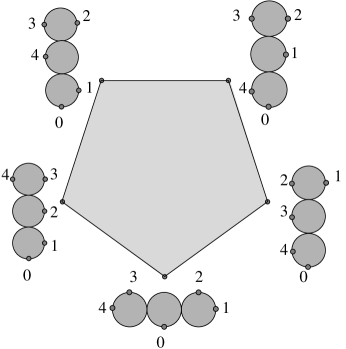
Figure 4. $\overline{\mathcal{R}}^{4}$

The moduli space of stable marked disks comes with a universal curve whose fibers over any isomorphism class of curves is the curve itself. That is, the universal curve $\overline{\mathcal{U}}^{d}$ is the space of isomorphism classes of tuples $[D,z_{1},\ldots,z_{n},z]$ where $(D,z_{1},\ldots,z_{n})$ is a stable $n$-marked disk and $z\in D$ is a possibly nodal or marked point. The topology on the universal curve is defined in a similar way to the moduli space of stable disks, and the map forgetting the additional point

$$\overline{\mathcal{U}}^{d}\to\overline{\mathcal{R}}^{d},\quad[D,z_{1},\ldots,z_{n},z]\mapsto[D,z_{1},\ldots,z_{n}]$$

is continuous with respect to these topologies.

Each moduli space of disks has the structure of a manifold with corners. Coordinates near each stratum are given by the gluing construction, as follows.

Theorem 4.6.

(Compatible tubular neighborhoods for associahedra) For integers $d\geq 2,m\geq 0$, each stratum $\mathcal{R}_{\Gamma}^{d}$ with $m$ nodes has an open neighborhood homeomorphic to $\mathcal{R}_{\Gamma}\times[0,\infty)^{m}$. The normal coordinates can be chosen compatibly in the sense that if $\Gamma<\Gamma^{\prime}$ and $\Gamma^{\prime}$ has $m^{\prime}$ nodes then the diagram

$$\begin{diagram}$$

commutes.

Sketch of proof.

Given a stable $n$-marked nodal disk $D$ with components $D_{0},\ldots,D_{r}$ with $m$ nodes $w_{1}^{\pm},\ldots,w_{m}^{\pm}$, let $\delta_{1},\ldots,\delta_{m}\in\mathbb{R}_{\geq 0}$ be a set of gluing parameters. Suppose that each node is equipped with local coordinates: holomorphic embeddings

$$\phi_{j}^{\pm}:(B^{+}_{\epsilon}(0),0)\to(D,w_{j}^{\pm})$$

where $B^{+}_{\epsilon}(0)\subset B_{\epsilon}(0)$ is the part of the $\epsilon$-ball around $0$ in the complex plane with non-negative imaginary part. The glued disk $G_{\delta}(D)$ is obtained by removing small balls around the $j$-th node and identifying points by the map $z\mapsto\delta_{j}/z$ for every gluing parameter that is non-zero. Suppose that one has for every point $r\in\mathcal{R}_{\Gamma}^{d}$ a set of such local coordinates varying smoothly in $r$. Then one obtains from the gluing construction a collar neighborhood as in the statement of the theorem.

To check the compatibility relation, suppose that $I\subset\{1,\ldots,m\}$ is a subset of the nodes and $\delta_{I}\in\mathbb{R}_{\geq 0}^{|I|}$ the corresponding gluing parameters. Starting with the disk above, glue together open balls around the nodes $w_{i}^{\pm},i\in I$ to obtain a disk $G_{\delta_{I}}(D)$, equipped with local coordinates near the unresolved nodes given by the local coordinates near the nodes of $D$, of combinatorial type $\Gamma^{\prime}$ with $m^{\prime}=m-|I|$ nodes. Suppose that a family of local coordinates near the nodes of $\mathcal{R}_{\Gamma^{\prime}}$ is given such that in a neighborhood of $\mathcal{R}_{\Gamma}$ the local coordinates are induced by those on $\mathcal{R}_{\Gamma}$ by gluing. In this case the collar neighborhoods for $\Gamma$ and $\Gamma^{\prime}$ are compatible in the sense that the diagram in the theorem commutes.

One may always choose the local coordinates to be given by gluing near the boundary, since the space of germs of local coordinates is convex. Indeed a map $\phi_{j}^{\pm}:(B^{+}_{\epsilon}(0),0)\to(D,w_{j}^{\pm})$ defines a local coordinate in some neighborhood of $0$ iff $D\phi_{j}^{\pm}(0)>0$, which is a convex condition. So we may assume that on each stratum $\mathcal{R}_{\Gamma}^{d}$ there is a family of local coordinates such that near any stratum $\mathcal{R}_{\Gamma^{\prime}}^{d}$ contained in the closure the local coordinates are those induced by $\mathcal{R}_{\Gamma^{\prime}}^{d}$ from gluing. This completes the proof. ∎

It follows that the stratified space $\overline{\mathcal{R}}^{d}$ is equipped with quilt data in the sense of Definition 2.17: each stratum comes with a collar neighborhood described by gluing parameters compatible with the lower dimensional strata.

The moduli spaces of marked disks admit forgetful morphisms to moduli spaces with fewer numbers of markings. For each $i=1,\ldots,d$, we have a forgetful morphism

(24) $$f_{i}:\overline{\mathcal{R}}^{d}\to\overline{\mathcal{R}}^{d-1},\quad[D,z_{1},\ldots,z_{n}]\mapsto[D,z_{1},\dots,z_{i-1},z_{i+1},\ldots,z_{n}]^{\operatorname{st}}$$

where the superscript $\operatorname{st}$ indicates the disk obtained from $D$ by collapsing unstable components. There is a well-known description of the forgetful map (in the context of Deligne-Mumford spaces) as the projection from the universal curve, developed in the case of closed curves by Knudsen [14, Sections 1,2]. In the case of disks, the universal curve $\overline{\mathcal{U}}^{d}$ has a fiber-wise boundary $\partial\mathcal{U}^{d}$ which splits as a union of intervals

$$\partial\mathcal{U}^{d}=(\partial\mathcal{U}^{d})_{0}\cup\ldots\cup(\partial\mathcal{U}^{d})_{d}$$

where $(\partial\mathcal{U}^{d})_{i}$ is the part of the boundary between the $i-1$-st and $i$-th marking, where $i$ is taken mod $d+1$. See Figure 5. The map $f_{i}$ naturally lifts to a continuous map

(25) $$\tilde{f}_{i}:\overline{\mathcal{R}}^{d}\to(\partial\mathcal{U}^{d-1})_{i},\quad[D,z_{1},\dots,z_{n}]\mapsto[D^{\operatorname{st}},z_{1},\dots,z_{i-1},z_{i+1},\ldots,z_{n},z_{i}^{\operatorname{st}}]$$

where $z_{i}^{\operatorname{st}}\in D^{\operatorname{st}}$ is the image of $z_{i}$ under the stabilization map $D\to D^{\operatorname{st}}$. A continuous inverse to $\tilde{f}_{i}$ is defined by inserting $z_{i}^{\operatorname{st}}$ in between $z_{i-1}$ and $z_{i+1}$, and creating an additional component if $z_{i}^{\operatorname{st}}$ is a nodal point of $D^{\operatorname{st}}$, showing that $\tilde{f}_{i}$ is a homeomorphism.

Figure 5. The part of the boundary between two markings

The forgetful maps induce the structure of fiber bundles on the moduli spaces with contractible fibers. Indeed the gluing construction identifies all nearby fibers $G_{\delta}D$ with the interval obtained by removing small disks around the nodes and identifying the endpoints:

(26) $$(\partial G_{\delta}D)_{i}=\left((\partial D)_{i}-\cup_{k=1}^{m}B_{\delta_{k}^{1/2}}(w_{k})\right)/\sim.$$

On the other hand the intervals on the right-hand side of (26) are homeomorphic to $(\partial D)_{i}$ itself, by extending a homeomorphism of the complement

$$(\partial D)_{i}-\cup_{k=1}^{m}B_{\delta_{k}^{1/2}}(w_{k})\to(\partial D)_{i}-\cup_{k=1}^{m}\{w_{k}\}$$

to the boundary. It follows that $f_{i}$ induces on $\overline{\mathcal{R}}^{d}$ the structure of a fiber bundle over $\overline{\mathcal{R}}^{d-1}$ with interval fibers. The discussion above shows by induction that the moduli space $\overline{\mathcal{R}}^{d}$ is a topological disk. (And it follows from the isomorphism with the associahedron that they are isomorphic, as decomposed spaces, to convex polytopes.)

4.3. Higher compositions

In this section we construct the higher composition maps on the Fukaya category of generalized Lagrangian branes. These are defined by family quilt invariants for families of surfaces with strip-like ends over the associahedra constructed in the following proposition:

Proposition 4.7.

(Existence of families of strip-like ends over the associahedra) For each $d\geq 2$ there exists a collection of families of quilted surfaces $\overline{\SS}^{d}$ with strip-like ends over $\overline{\mathcal{R}}^{d}$ with the property that the restriction $\SS^{d}_{\Gamma}$ of the family to a stratum $\mathcal{R}_{\Gamma}^{d}$ that is isomorphic to a product of $\mathcal{R}^{i_{j}},j=1,\ldots,k$ is a product of the corresponding families $\SS^{i_{j}}$, and collar neighborhoods of $\SS^{d}_{\Gamma}$ are given by gluing along strip-like ends.

Proof.

The claim follows by induction using Theorem 1.3 applied to the stratified space $\overline{\mathcal{R}}^{d}$ constructed in Theorem 4.6, starting from the case of three-marked disk where we choose a genus zero surface with strip-like ends. ∎

The compactness and regularity properties of the family moduli spaces in the previous section combine to the following statement, in the case of the constructed families over the associahedra:

Proposition 4.8.

(Existence of compact families of holomorphic quilts over the associahedra) Let $M$ be a symplectic background, and for $d\geq 2$ let $\underline{L}^{0},\ldots,\underline{L}^{d}$ be admissible generalized Lagrangian branes in $M$. For generic choices of inductively-chosen perturbation data $\underline{J},\underline{K}$ and $d\geq 2$

1. the moduli space of pseudoholomorphic quilts $\mathcal{M}^{d}_{0}$ of dimension zero in $M$ with boundary in $\underline{L}^{j},j=0,\ldots,d$ is compact, and

2. the one-dimensional component $\overline{\mathcal{M}}^{d}_{1}$ has a compactification as a one-manifold with boundary the union

   $$\partial\overline{\mathcal{M}}^{d}_{1}=\bigcup_{\Gamma}{\mathcal{M}}^{d}_{\Gamma,1}$$

   of strata $\mathcal{M}^{d}_{\Gamma,1}$ of $\overline{\mathcal{M}}^{d}_{1}$ corresponding to trees with two vertices (where either (1) $\Gamma$ is stable with two vertices, or (2) $\Gamma$ is unstable and corresponds to bubbling of a Floer trajectory).

A similar statement holds for $d=1$, using moduli spaces of unparametrized Floer trajectories.

Proof.

For $d\geq 2$, regular perturbation data exist by the recursive application of Theorem 1.4 to the family of quilted surfaces $\overline{\SS}^{d}\to\overline{\mathcal{R}}^{d}$ constructed in Proposition 4.7; the perturbation over the boundary of $\overline{\SS}^{d}$ is that of product form for the lower-dimensional associahedra. The description of the boundary follows from Theorem 3.7. ∎

Theorem 1.5 gives chain-level family quilt invariants associated to the family over the associahedron defined in Theorem 4.8. The $A_{\infty}$ composition maps are related to these by additional signs:

Definition 4.9.

(Higher composition maps for the extended Fukaya category) For $d\geq 2$ let $\overline{\SS}^{d}\to\overline{\mathcal{R}}^{d}$ be the family of surfaces with strip-like ends over the associahedron $\overline{\mathcal{R}}^{d}$ constructed in Theorem 4.7 and $\Phi_{\overline{\SS}^{d}}$ the associated family quilt invariants. Given objects $\underline{L}^{0},\ldots,\underline{L}^{d}$ define

$$\mu^{d}:\operatorname{Hom}(\underline{L}^{0},\underline{L}^{1})\times\ldots\times\operatorname{Hom}(\underline{L}^{d-1},\underline{L}^{d})\to\operatorname{Hom}(\underline{L}^{0},\underline{L}^{d})$$

by

(27) $$\mu^{d}(\langle{\underline{x}_{1}}\rangle,\ldots,\langle{\underline{x}_{d}}\rangle)=(-1)^{\heartsuit}\Phi_{\overline{\SS}^{d}}(\langle{\underline{x}_{1}}\rangle,\ldots,\langle{\underline{x}_{d}}\rangle)$$

where

(28) $$\heartsuit={\sum_{i=1}^{d}i|\underline{x}_{i}|}.$$

Theorem 4.10.

Let $M$ be a symplectic background, and $\mu^{d}$ for $d\geq 1$ the maps defined in (27) for some choice of family of surfaces of strip-like ends and perturbation data. Then the maps $\mu^{d},d\geq 1$ define an $A_{\infty}$ category ${\operatorname{Fuk}^{\includegraphics[height=5.05942pt]{sharp.eps}}}(M)$.

Proof.

Without signs the theorem holds for $d\geq 2$ by the description of the ends of the one-dimensional moduli spaces in Theorem 4.8. To check the signs in the $A_{\infty}$ associativity relation, suppose for simplicity that all generalized Lagrangian branes are length one. Let $x_{j}\in\mathcal{I}(\underline{L}^{j},\underline{L}^{j+1})$ for $j=0,\ldots,d$ indexed mod $d+1$ and $\overline{\mathcal{M}}^{d}(x_{0},\ldots,x_{d})$ the moduli space of quilts with limits $x_{0},\ldots,x_{d}$ along the strip-like ends. Consider the gluing map constructed in Ma’u [21, Theorem 1]

(29) $$\mathcal{M}^{m}({y},{x}_{n+1},\ldots,{x}_{n+m})_{0}\times\mathcal{M}^{d-m+1}({x}_{0},{x}_{1},\ldots,{y},\ldots,{x}_{d})_{0}\to\mathcal{M}^{d}({x}_{0},\ldots,{x}_{d})_{1}.$$

For any intersection point $x_{j}$ let $\mathcal{D}^{+}_{x_{j}}$ denote the determinant line associated to $x_{j}$ in [41, Equation (40)] of the Fredholm operator on the once-punctured disk associated to a choice of path from $T_{x_{j}}\underline{L}^{j-1}$ and $T_{x_{j}}\underline{L}^{j}$ to a collection of Lagrangians of split form in $T_{x_{j}}\underline{M}_{j}$ (where here $\underline{M}_{j}$ denotes the collection of patches meeting the $j$-th end). The determinant lines $\mathcal{D}^{-}_{x_{j}}$ is defined similarly, but with an added determinant $\operatorname{det}(T_{x_{j}}\underline{L}^{j})$ of the Lagrangians meeting the end. By assumption, the orientations on $\mathcal{D}^{\pm}_{x_{j}}$ are defined so that the tensor product

$$\mathcal{D}^{-}_{x_{j}}\otimes\mathcal{D}^{+}_{x_{j}}\cong\mathbb{R}$$

is canonically trivial. By deforming the parametrized linear operator to the linearized operator plus a trivial operator, and bubbling off marked disk on each strip like end we may identify via [41, Equation (40)]

(30) $$\operatorname{det}(T{\mathcal{M}}^{d}(x_{0},\ldots,x_{d}))\to\operatorname{det}(T\mathcal{R}^{d})\mathcal{D}^{+}_{x_{0}}\mathcal{D}^{-}_{x_{1}}\ldots\mathcal{D}^{-}_{x_{d}}.$$

After this identification the gluing map (29) takes the form (omitting tensor products from the notation to save space)

(31) $$\operatorname{det}(\mathbb{R})\operatorname{det}(T\mathcal{R}^{m})\mathcal{D}^{+}_{y}\mathcal{D}^{-}_{x_{n+1}}\ldots\mathcal{D}^{-}_{x_{n+m}}\operatorname{det}(T\mathcal{R}^{d-m+1})\mathcal{D}^{+}_{x_{0}}\mathcal{D}^{-}_{x_{1}}\ldots\mathcal{D}^{-}_{y}\ldots\mathcal{D}^{-}_{x_{d}}.$$

To determine the sign of this map, first note that the gluing map

$$(0,\epsilon)\times\mathcal{R}^{m}\times\mathcal{R}^{d-m+1}\to\mathcal{R}^{d}$$

on the associahedra is given in coordinates (using the automorphisms to fix the location of the first and second point in $\mathcal{R}^{m}$ to equal $0$ resp. $1$ and $\mathcal{R}^{d-m+1}$) by

(32) $$(\delta,(z_{3},\ldots,z_{m}),(w_{3},\ldots,w_{d-m+1}))\\ \to(w_{3},\ldots,w_{n+1},w_{n+1}+\delta,w_{n+1}+\delta z_{3},\ldots,w_{n+1}+\delta z_{m},w_{n+2},\ldots,w_{d-m}).$$

This map acts on orientations by a sign of $-1$ to the power

(33) $$(m-1)(n-1).$$

These signs combine with the contributions

(34) $$\sum_{k=1}^{n}k|x_{k}|+(n+1)|y|+\sum_{k=n+m+1}^{d}(k-m+1)|x_{k}|+\sum_{k=n+1}^{m}(k-n)|x_{k}|$$

in the definition of the structure maps, and a contribution

(35) $$(d-m+1)m+m\left(|y|+\sum_{i\geq n}|x_{i}|\right)$$

from permuting the determinant lines $\mathcal{D}_{x_{j}}^{-},j=n+1,\dots,n+m,\mathcal{D}_{y}^{+}$ with $\operatorname{det}(T\mathcal{R}^{d-m+1})$ and permuting these determinant lines with the $\mathcal{D}_{x_{i}}^{-},i\leq n,\mathcal{D}_{y}^{-}$. On the other hand, the sign in the $A_{\infty}$ axiom contributes

(36) $$\sum_{k=1}^{n}(|x_{k}|+1)$$

Combining the signs (33), (34), (35), (36) one obtains mod $2$

(37) $$\left(mn+n+m\right)+\left(\sum_{k=1}^{n}k|x_{k}|+(n+1)|y|+\sum_{k=n+m+1}^{d}(k-m+1)|x_{k}|+\sum_{k=n+1}^{n+m}(k-n)|x_{k}|\right)\\ +(d-m+1)m+m\left(|y|+\sum_{i\leq n}|x_{i}|\right)+\sum_{k=1}^{n}(|x_{k}|+1)\\ \equiv(mn+m+n)+\sum_{k=1}^{d}k|x_{k}|+(n+1)|y|+\sum_{k=n+m+2}^{d}(m-1)|x_{k}|+\sum_{k=n+1}^{n+m}n|x_{k}|\\ +(d-m+1)m+m\left(d+\sum_{i\geq n+m+1}|x_{i}|\right)+\sum_{k=1}^{n}|x_{k}|+n$$

(38) $$\equiv mn+m+\sum_{k=1}^{d}k|x_{k}|+|y|+\sum_{k=n+m+2}^{d}|x_{k}|+nm+(d-m+1)m+md+\sum_{k=1}^{n}|x_{k}|+n\\ \equiv m+\sum_{k=1}^{d}k|x_{k}|+\sum_{k=n+1}^{n+m}|x_{k}|+m+\sum_{k=n+m+2}^{d}|x_{k}|+\sum_{k=1}^{n}|x_{k}|$$

which is congruent mod $2$ to

(39) $$\sum_{k=1}^{d}(k+1)|x_{k}|.$$

Since (39) is independent of $n,m$, the $A_{\infty}$ -associativity relation (77) follows. ∎

Remark 4.11.

(Units) Cohomological units are constructed in [42]. The unit for $\underline{L}$ is defined by counting perturbed pseudoholomorphic once-punctured disks with boundary in $\underline{L}$. That is, the unit is the relative invariant associated to the quilt obtained from the once-punctured disk by attaching sequence of strips so that the boundaries lie in the Lagrangian correspondences in $\underline{L}$.

4.4. The Maslov index two case

The definitions of the previous sections extend to the case of Maslov index two Lagrangians, once one fixes a total disk invariant as in Oh [25, Addendum]. Given a Lagrangian $L\subset M$ and a point $\ell\in L$, we denote by $\mathcal{M}_{1}^{2}(L,J,\ell)$ the moduli space of Maslov index two holomorphic maps $u:(D,\partial D)\to(X,L)$ mapping $1\in D$ to $\ell\in L$.

Proposition 4.12.

(Disk invariant of a Lagrangian) For any $\ell\in L$ there exists a comeager subset $\mathcal{J}^{\rm reg}(\ell)\subset\mathcal{J}(M,\omega)$ such that $\mathcal{M}_{1}^{2}(L,J,\ell)$ is cut out transversally. Any relative spin structure on $L$ induces an orientation on $\mathcal{M}_{1}^{2}(L,J,\ell)$. Letting $\epsilon:\mathcal{M}_{1}^{2}(L,J,\ell)\to\{\pm 1\}$ denote the map comparing the given orientation to the canonical orientation of a point, the disk number of $L$,

$$w(L):=\sum_{[u]\in\mathcal{M}_{1}^{2}(L,J,\ell)}\epsilon([u]),$$

is independent of $J\in J^{{\operatorname{reg}}}(\ell)$ and $\ell\in L$.

See Oh [25, Addendum] for the proof. The quilted Floer operator in the minimal Maslov index two case satisfies the following relation involving the disk invariant above. Let $\underline{L}=(L_{j(j+1)})_{j=0,\ldots,r}$ be a cyclic generalized Lagrangian brane between symplectic backgrounds $M_{j},j=0,\ldots,r$. Let

$$\mathcal{J}_{t}(\underline{L}):=\prod_{j=0}^{r}C^{\infty}([0,\delta_{j}],\mathcal{J}(M_{j},\omega_{j}))$$

denote the space of time-dependent almost complex structures on strips with width $\delta_{j}$.

Theorem 4.13.

(Quilted Floer cohomology) For any $\underline{H}\in\operatorname{Ham}(\underline{L})$, widths $\underline{\delta}=(\delta_{j}>0)_{j=0,\ldots,r}$, and $\underline{J}$ in a comeager subset $\mathcal{J}^{{\operatorname{reg}}}_{t}(\underline{L},\underline{H})\subset\mathcal{J}_{t}(\underline{L})$, the Floer differential $\partial:CF(\underline{L})\to CF(\underline{L})$ satisfies

$$\partial^{2}=w(\underline{L})\operatorname{Id},\qquad w(\underline{L})=\sum_{j=0}^{r}w(L_{j(j+1)}).$$

The pair $(CF(\underline{L}),\partial)$ is independent of the choice of $\underline{H}$ and $\underline{J}$, up to cochain homotopy.

Proof.

We sketch the proof, following Oh [25, Addendum] in the case of $\mathbb{Z}_{2}$ coefficients. For any $\underline{x}_{\pm}\in\mathcal{I}(\underline{L})$, the zero dimensional component $\mathcal{M}(\underline{x}_{-},\underline{x}_{+})_{0}$ of Floer trajectories is a finite set. As in [25, Proposition 4.3] the one-dimensional component $\mathcal{M}(\underline{x}_{-},\underline{x}_{+})_{1}$ is smooth, but the “compactness modulo breaking” does not hold in general: Apart from the breaking of trajectories, a sequence of Floer trajectories of Maslov index $2$ could in the Gromov compactification converge to a constant trajectory and either a sphere bubble of Chern number one or a disk bubble of Maslov number two. All other bubbling effects are excluded by monotonicity. Thus failure of “compactness modulo breaking” can occur only when $\underline{x}_{-}=\underline{x}_{+}$.

The proof follows from the claim that each one-dimensional moduli space $\mathcal{M}(\underline{x},\underline{x})_{1}$ of self-connecting trajectories has a compactification as a one-dimensional manifold with boundary

$$\partial\overline{\mathcal{M}(\underline{x},\underline{x})_{1}}\;\cong\;\bigcup_{\underline{y}\in\mathcal{I}(\underline{L})}\bigl{(}\mathcal{M}(\underline{x},\underline{y})_{0}\times\mathcal{M}(\underline{y},\underline{x})_{0}\bigr{)}\;\cup\;\bigcup_{j=0,\ldots,r}\mathcal{M}_{1}^{2}(L_{j(j+1)},J_{j(j+1)},\{(x_{j},x_{j+1})\})^{-}$$

and that furthermore the orientations on these moduli spaces induced by the relative spin structures are compatible with the inclusion of the boundary. Here $\mathcal{M}_{1}^{2}(\ldots)^{-}$ denotes the moduli space $\mathcal{M}_{1}^{2}(\ldots)$ with orientation reversed. The subset $\mathcal{J}^{{\operatorname{reg}}}_{t}(\underline{L};\underline{H})$ consists of collections of time-dependent almost complex structures $J_{j}:[0,\delta_{j}]\to\mathcal{J}(M_{j},\omega_{j})$ for which all $\mathcal{M}(\underline{x}_{-},\underline{x}_{+})$ are smooth and the universal moduli spaces of spheres $\mathcal{M}_{1}^{1}(M_{j},\{J_{j}(t)\}_{t\in[0,\delta_{j}]},\{x_{j}\})$ are empty for all $\underline{x}=(x_{j})_{j=0,\ldots,r}\in\mathcal{I}(\underline{L})$. This choice excludes the Gromov convergence to a constant trajectory and a sphere bubble. We now restrict to those $\underline{J}\in\mathcal{J}^{{\operatorname{reg}}}_{t}(\underline{L};\underline{H})$ such that

$$J_{j(j+1)}:=(-J_{j}(\delta_{j}))\oplus J_{j+1}(0)\in\mathcal{J}^{\rm reg}(L_{j(j+1)},\{(x_{j},x_{j+1})\})$$

for all $\underline{x}\in\mathcal{I}(\underline{L})$ and $j=0,\ldots,r$. This still defines a comeager subset in $\mathcal{J}_{t}(\underline{L})$.

To finish the proof of the claim we use a gluing theorem of non-transverse type for pseudoholomorphic maps with Lagrangian boundary conditions. The required gluing theorem can be adapted from [22, Chapter 10] as follows: Replace $\underline{L}$ with its translates under the Hamiltonian flows of $\underline{H}$, so that the Floer trajectories are unperturbed $J_{j}$-holomorphic strips (where the $J_{j}$ have suffered some Hamiltonian transformation, too). Pick $[v_{j(j+1)}]\in\mathcal{M}_{1}^{2}(L_{j(j+1)},J_{j(j+1)},\{(x_{j},x_{j+1})\})$ and a representative $v_{j(j+1)}$. The gluing construction gives a map

(40) $$(T,\infty)\longrightarrow\mathcal{M}(\underline{x},\underline{x})_{1}$$

to the moduli space of parametrized Floer trajectories of index $2$, where $T\gg 0$ is a real parameter. This construction first identifies $v_{j(j+1)}$ with a map from the half space $\mathbb{H}\cong D\setminus\{1\}$ to $M_{j}^{-}\times M_{j+1}$. For the pregluing choose a gluing parameter $\tau\in(T,\infty)$. Outside of a half disk of radius $\frac{1}{2}\tau^{1/2}$ around $0$, interpolate the map to the constant solution $(x_{j},x_{j+1})$ outside of the half disk of radius $\tau^{1/2}$ using a slowly varying cutoff function in submanifold coordinates of $L_{j(j+1)}\subset M_{j}^{-}\times M_{j+1}$ near $(x_{j},x_{j+1})$. Then rescale this map by $\tau$ to a half-disk of radius $\tau^{-1/2}$ centered around $0$ in the strip $\mathbb{R}\times[0,\tau^{-1/2})$, again extended constantly. The components give an approximately $J_{j+1}$-holomorphic map $u_{j+1}:\mathbb{R}\times[0,\tau^{-1/2})\to M_{j+1}$ and, after reflection, an approximately $J_{j}$-holomorphic map $u_{j}:\mathbb{R}\times(\delta_{j}-\tau^{-1/2},\delta_{j}]\to M_{j}$. For $T\geq\max\{\delta_{j}^{-2},\delta_{j+1}^{-2}\}$ these strips can be extended to width $\delta_{j}$ resp. $\delta_{j+1}$. Together with the constant solutions $u_{\ell}\equiv x_{\ell}$ for $\ell\not\in\{j,j+1\}$ we obtain a tuple

$$\underline{u}=(u_{\ell}:\mathbb{R}\times[0,\delta_{\ell}]\to M_{\ell})_{\ell=0,\ldots,r}$$

that is an approximate Floer trajectory. An application of the implicit function theorem gives an exact solution for $T$ sufficiently large. The uniqueness part of the implicit function theorem gives that $[v_{j(j+1)}]$ is an isolated limit point of $\mathcal{M}(\underline{x},\underline{x})_{1}$, so that $\overline{\mathcal{M}}(\underline{x},\underline{x})_{1}$ is a one-dimensional manifold with boundary in a neighborhood of the nodal trajectory with disk bubble $[v_{j(j+1)}]$.

It remains to examine the effect of the gluing on orientations for which we need to recall the construction of orientations in [41]. Choose a parametrization

$$[T,\infty]\to\overline{\mathcal{M}}(\underline{x},\underline{x})_{1},\quad\infty\mapsto[v_{j(j+1)}]$$

homotopic to the gluing map. Now the action on orientations is given by the action on local homology groups, and homotopic maps induce the same action. So by replacing the gluing map with this parametrization we may assume that the gluing map is an embedding. The moduli space $\mathcal{M}_{1}^{2}(L_{j(j+1)},J_{j(j+1)},\{(x_{j},x_{j+1})\})$ has orientation at $[u]$ induced by determinant line $\operatorname{det}(D_{u})$ and the determinant of the infinitesimal automorphism group $\operatorname{aut}(\mathbb{R}\times[0,1])\cong\mathbb{R}$. On the other hand, the orientation on $\mathcal{M}_{1}^{2}(L_{j(j+1)},J_{j(j+1)},\{(x_{j},x_{j+1})\})$ is induced by the orientation of the determinant line $\operatorname{det}(D_{v_{j(j+1)}})$ and the determinant line of the automorphism group $\operatorname{Aut}(D,\partial D,1)\cong(0,\infty)\times\mathbb{R}$. The gluing map induces an orientation-preserving isomorphism of determinant lines $\operatorname{det}(D_{u})\to\operatorname{det}(D_{v_{j(j+1)}})$ by [41]. Under gluing the second factor in $\operatorname{Aut}(D,\partial D,1)$ agrees with the translation action on $\mathbb{R}\times[0,1]$. On the other hand, the first factor agrees approximately with the gluing parameter, in the sense that gluing in a dilation of $v_{j(j+1)}$ by a small constant $\rho>0$ using gluing parameter $\tau$ is approximately the same as gluing in $v_{j(j+1)}$ with gluing parameter $\tau\rho$. Thus $v_{j(j+1)}$ represents a boundary point of $\overline{\mathcal{M}}(\underline{x},\underline{x})_{1}$ with the opposite of the induced orientation from the interior. Summing over the boundary of the one-dimensional manifold $\partial\overline{\mathcal{M}}(\underline{x},\underline{x})_{1}$ proves that $\partial^{2}-\sum_{j=0}^{r}w(L_{j(j+1)})\operatorname{Id}=0$. The proof that two choices lead to cochain-homotopic pairs $(CF(\underline{L}),\partial)$ is given in [37]. ∎

Remark 4.14.

(Floer theory of a pair of Lagrangians) In the special case $\underline{L}=(L_{0},L_{1})$ of a cyclic correspondence consisting of two Lagrangian submanifolds $L_{0},L_{1}\subset M$ we have $w(\underline{L})=w(L_{0})-w(L_{1})$. Indeed the $-J_{1}$-holomorphic discs with boundary on $L_{1}\subset M^{-}\times\{\operatorname{pt}\}$ are identified with $J_{1}$-holomorphic discs with boundary on $L_{1}\subset M$ via a reflection of the domain. This reflection is orientation reversing for the moduli spaces. In particular, the differential for a monotone pair $\underline{L}=(L,\psi(L))$ with any symplectomorphism $\psi\in\operatorname{Symp}(M)$ always squares to zero, since $w(L)=w(\psi(L))$.

Following Sheridan [30], for each integer $w\in\mathbb{Z}$ define the generalized Fukaya category ${\operatorname{Fuk}^{\includegraphics[height=5.05942pt]{sharp.eps}}}(M,w)$ whose objects are generalized Lagrangians $\underline{L}$ whose total disk invariant is $w(\underline{L})=w$, and whose morphisms are the quilted Floer cochain groups defined above.

Theorem 4.15.

Let $M$ be a symplectic background, $w\in\mathbb{Z}$ an integer and $\mu^{d}$ for $d\geq 1$ the maps defined in (27) for some choice of family of surfaces of strip-like ends and perturbation data. Then the maps $\mu^{d},d\geq 1$ define an $A_{\infty}$ structure on ${\operatorname{Fuk}^{\includegraphics[height=5.05942pt]{sharp.eps}}}(M,w)$.

Proof.

The possibility of disk bubbling occurs only the definition of $\mu_{1}^{2}$, since it is only in this case that there exist holomorphic quilts in a moduli space that is not of expected dimension (the constant trajectories). The proof is therefore the same as in the case of Maslov number at least three, with the added requirement that the perturbation data on the ends makes the disks in the definition of the disk invariant regular. ∎

5. Functors for Lagrangian correspondences

In this section we construct $A_{\infty}$ functors associated to any admissible Lagrangian correspondence equipped with a brane structure.

5.1. Moduli of stable quilted disks

The multiplihedron is a polytope introduced by Stasheff in [33] which plays the same role in the theory of $A_{\infty}$ morphisms as the associahedron does for $A_{\infty}$ algebras.

Definition 5.1.

For $d\geq 1$, the complex $\mathcal{K}^{d,0}$ is a compact cell complex of dimension $d-1$ whose vertices correspond to the ways of maximally bracketing $d$ formal variables $a_{1},\ldots,a_{d}$ and applying a formal operation $h$. The complex $\mathcal{K}^{d,0}$ is defined recursively as the cone over the union of products of lower-dimensional spaces $\mathcal{K}^{e}$ and $\mathcal{K}^{f,0}$. [33].

Example 5.2.

1. (Second multiplihedron) The second multiplihedron $\mathcal{K}^{2,0}$ is homeomorphic to a closed interval with end points corresponding to the expressions $h(a_{1}a_{2})$ and $h(a_{1})h(a_{2})$.

2. (Third multiplihedron) The multiplihedron $\mathcal{K}^{3,0}$ is homeomorphic to a hexagon shown in Figure 6, with vertices corresponding to the expressions $h((a_{1}a_{2})a_{3})$, $h(a_{1}(a_{2}a_{3}))$, $h(a_{1})h(a_{2}a_{3})$, $h(a_{1}a_{2})h(a_{3})$, $(h(a_{1})h(a_{2}))h(a_{3})$, $h(a_{1})(h(a_{2})h(a_{3}))$.

Figure 6. Vertices of $\mathcal{K}^{3,0}$

We review from [20] the realization of the multiplihedron as the moduli space of stable nodal quilted disks with marked points.

Definition 5.3.

(Quilted disks) Let $d\geq 2$. A quilted disk with $d+1$ markings is a tuple $(D,C,z_{0},z_{1}\ldots,z_{d})$ where

1. $D$ is a holomorphic disk, which can be taken to be the closed unit disk in $\mathbb{C}$.

2. $C$ is a circle in $D$ with unique intersection point $C\cap\partial D=\{z_{0}\}$ equal to the $0$-th marking. That is, if $D$ is identified with a disk in $\mathbb{C}$ then $C$ is a circle in $D$ tangent to $\partial D$ at $z_{0}$.

3. $(z_{0},z_{1},\ldots,z_{d})$ is a tuple of distinct points in $\partial D$ whose cyclic order is compatible with the orientation of $\partial D$.

An isomorphism of marked quilted disks from $(D,C,z_{0},z_{1}\ldots,z_{d})$ to $(D^{\prime},C^{\prime},z^{\prime}_{0},z^{\prime}_{1}\ldots,z^{\prime}_{d})$ is a holomorphic isomorphism preserving the quiltings and markings:

$$\psi:D\to D^{\prime},\quad\psi(C)=C^{\prime},\quad\psi(z_{j})=z_{j}^{\prime},\quad j=0,\ldots,d.$$

The space of isomorphism classes of marked quilted disks admits a natural compactification by stable quilted disks, defined as follows.

Definition 5.4.

1. (Colored trees) A colored tree is a pair $(\Gamma,\operatorname{Edge}_{\infty}(\Gamma))$ consisting of a tree $\Gamma=(\operatorname{Vert}(\Gamma),\operatorname{Edge}(\Gamma))$ with semiinfinite edges $\operatorname{Edge}_{\infty}(\Gamma)\subset\operatorname{Edge}(\Gamma)$ labelled $z_{0},\dots,z_{d}$ equipped with a distinguished set of colored vertices $\operatorname{Vert}^{(1)}(\Gamma)$ with the following property:

   • For each $j=1,\ldots,d,$ the unique shortest path in $\Gamma$ from the semi-infinite root edge marked $z_{0}$ to the semi-infinite edge $z_{j}$ crosses exactly one colored vertex.

   A colored tree is stable if each colored resp. uncolored vertex has valence at least two resp. three.

2. (Nodal quilted disks) A nodal $(d+1)$-marked quilted disk $\underline{S}$ of combinatorial type equal to a colored tree $\Gamma$ is a collection $D_{i},i=1,\ldots,a$ and $(D_{i}^{\prime},C_{i}^{\prime}),i=1,\ldots,b$ of quilted and unquilted marked disks, identified at pairs of points on the boundary $w_{k}^{-}\in\partial D_{i^{-}(k)},w_{k}^{+}\in\partial D_{i^{+}(k)}$ distinct from each other and the interior circles, together with a collection $z_{0},\ldots,z_{d}$ of distinct smooth points on the boundary of $D=\sqcup_{i=1}^{a}D_{i}\sqcup\sqcup_{i=1}^{b}D_{i}^{\prime}$ such that the graph obtained by replacing disks resp. quilted disks with unquilted resp. quilted vertices is the given colored tree $\Gamma$. An isomorphism of nodal marked quilted disks $D,D^{\prime}$ with the same combinatorial type $\Gamma$ is a collection of complex isomorphisms $\phi_{v}:D_{v}\to D^{\prime}_{v},v\in\operatorname{Vert}(\Gamma)$ of the corresponding disk components, identifying nodal points, marked points, and/or inner circles.

3. (Stable quilted disks) A nodal quilted disk is stable if and only if it has no automorphisms, or equivalently the corresponding colored tree is stable. More concretely, a nodal quilted disk is stable if and only if each quilted disk component $(D_{i},C_{i})$ contains at least $2$ singular or marked points

   $$D_{i}\text{ \ quilted \ }\implies\#\{z_{k}\in D_{i}\}+\#\{w_{j}\in D_{i}\}\geq 2$$

   and each non-quilted disk component $D_{i}$ contains at least $3$ singular or marked points

   $$D_{i}\text{ \ unquilted \ }\implies\#\{z_{k}\in D_{i}\}+\#\{w_{j}\in D_{i}\}\geq 3.$$

   Equivalently $(D,C,\underline{z})$ has no non-trivial automorphisms:

   $$\#\operatorname{Aut}(D,C,\underline{z})=1.$$

We introduce the following notations for moduli spaces of quilted disks. Denote by $\mathcal{R}^{d,0}_{\Gamma}$ for the set of isomorphism classes of combinatorial type $\Gamma$. The moduli space $\overline{\mathcal{R}}^{d,0}$ is the union of $\mathcal{R}^{d,0}_{\Gamma}$ over combinatorial types $\Gamma$. As before in (24), forgetting a marking and stabilizing produces a fiber bundle $f_{i}:\mathcal{R}^{d,0}\to\mathcal{R}^{d-1,0}$ with interval fibers isomorphic to the part of the boundary between the $i-1$ and $i+1$-st markings. This implies by induction that $\overline{\mathcal{R}}^{d,0}$ is a topological disk. There is also a forgetful map

(41) $$f:\overline{\mathcal{R}}^{d,0}\to\overline{\mathcal{R}}^{d}$$

forgetting a seam which is, restricted to any stratum $\mathcal{R}^{d,0}_{\Gamma}$, a fiber bundle with open interval fibers. For example, the top-dimensional stratum $\mathcal{R}^{d,0}$ may be identified with the space of tuples $(w_{2}<\ldots<w_{d})$ by fixing $w_{1}=0$ and taking the seam to be given by $\operatorname{Im}(z)=1$ in $\mathcal{H}\cong D-\{1\}$. The forgetful morphism for forgetting the seam is then in coordinates

$$(w_{2}<\ldots<w_{d})\to(w_{3}/w_{2}<\ldots<w_{d}/w_{2}).$$

This map is smooth and surjective with fiber the space of quilted disks represented by tuples $[0,\lambda,\lambda w_{3}/w_{2},\ldots,\lambda w_{d}/w_{2}]$.

Example 5.5.

(The third multiplihedron) The moduli space $\overline{\mathcal{R}}^{3,0}$ is the hexagon shown in Figure 7. The picture shows how the interior circle on the open stratum can “bubble off” into the bubble disks on the boundary.

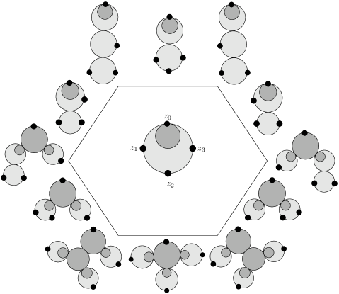
Figure 7. $\overline{\mathcal{R}}^{3,0}$

The local structure of the moduli space of quilted disks is described as follows, see Ma’u-Woodward [20].

Definition 5.6.

(Balanced gluing parameters) A collection of gluing parameters

$$\delta:\operatorname{Edge}_{<\infty}(\Gamma)\to[0,\infty)$$

is balanced if the following condition holds: for each pair $v_{1},v_{2}\in\operatorname{Vert}^{(1)}(\Gamma)$ of colored vertices, let $\gamma_{12}$ denote the shortest path in $\Gamma$ from $v_{1}$ to $v_{2}$. Then the relation

(42) $$\prod_{e\in\gamma_{12}}\delta(e)^{\pm 1}=1,\quad\forall v_{1},v_{2}\in\operatorname{Vert}^{(1)}(\Gamma)$$

holds where the sign is $+1$ resp. $-1$ if the edge points towards resp. away from the root edge.

The following theorem describes the local structure of the moduli space of quilted disks near any stratum. Let $Z_{\Gamma}\subset\operatorname{Map}(\operatorname{Edge}_{<\infty}(\Gamma),\mathbb{R}_{\geq 0})$ be the set of balanced gluing parameters from Definition 5.6.

Theorem 5.7.

(Existence of compatible tubular neighborhoods) For any integer $d\geq 1$ there exists a collection of open neighborhoods $U_{\Gamma}$ of $0$ in $Z_{\Gamma}$ and collar neighborhoods

$$G_{\Gamma}:\mathcal{R}_{\Gamma}^{d,0}\times U_{\Gamma}\to\overline{\mathcal{R}}^{d,0}$$

satisfying the following compatibility property: If $\mathcal{R}^{d,0}_{\Gamma^{\prime}}$ is contained in the closure of $\mathcal{R}^{d,0}_{\Gamma}$ and the local coordinates on $\mathcal{R}^{d,0}_{\Gamma}$ are induced via the gluing construction from those on $\mathcal{R}^{d,0}_{\Gamma^{\prime}}$ then the diagram

$$\begin{diagram}$$

commutes.

Sketch of proof.

The proof uses a version of the gluing construction for nodal disks to the quilted case. Let $D$ be a stable nodal quilted disk and $\delta\in Z_{\Gamma}$. The glued disk $G_{\delta}(D)$ is defined as follows. For each component $D_{j}$, let $w_{j}$ be the node connecting the disk with component containing the root marking $z_{0}$, or $z_{0}$ if $D_{j}$ is that component. We assume that for each $D_{j}$ an identification of $D_{j}-\{w_{j}\}$ with half-space $\mathcal{H}=\{\operatorname{Im}(z)\geq 0\}$ has been fixed. Such an identification is given by fixing two additional markings or nodes for an unquilted component, or one additional marking or node and the seam of the quilt as the line $C=\{\operatorname{Im}(z)=1\}$. Note that the space of such coordinates is convex.

1. (Unquilted case) In the case of a node not meeting any seam of a quilted disk corresponding to a gluing parameter $\gamma_{j}$, remove small balls around the node and glue together small annuli around the nodes using the map $z\mapsto\gamma_{j}z$. (Note the coordinate on the component “further away from $z_{0}$” is already inverted.)

2. (Quilted case) In the case of several nodes meeting seams of quilted disks, remove small balls around the nodes, glue together annuli around the nodes using the map $z\mapsto\gamma_{j}z$. Define the seam on the glued component is $C=\{\operatorname{Im}(z)=\gamma_{j}\}$ independent of $j$ by the relation on the gluing parameters.

The collar neighborhoods of the strata are given by the following global version of the gluing construction of the previous paragraph. Suppose that for each point $r\in\mathcal{R}^{d,0}_{\Gamma}$ a collection of local coordinates as above is given varying smoothly in $r$. Let $U_{\Gamma}$ be a neighborhood of $0$ in $Z_{\Gamma}$. Construct a collar neighborhood $G_{\Gamma}:\mathcal{R}_{\Gamma}^{d,0}\times U_{\Gamma}\to\overline{\mathcal{R}}^{d,0}$ by mapping each disk to the isomorphism class of the corresponding glued disk. Since the space of coordinates on the disks is contractible, we may assume that we have chosen local coordinates so that whenever a point $r\in\mathcal{R}^{d,0}_{\Gamma}$ is in the image of such a gluing map from $\mathcal{R}^{d,0}_{\Gamma^{\prime}}$, the local coordinates are those induced from $\mathcal{R}^{d,0}_{\Gamma^{\prime}}$. ∎

Thus the moduli space of quilted disks is equipped with quilt data as in Definition 2.17: each stratum comes with a collar neighborhood described by gluing parameters compatible with the lower dimensional strata. The space of gluing parameters is the positive real part of an affine toric variety by [24, 4.12], and in particular, is isomorphic as a decomposed space to a convex polyhedral cone. Thus the moduli of quilted disks is a locally polyhedral stratified space, and in particular there exists a collar neighborhood of the boundary.

Remark 5.8.

(Orientations) Orientations on $\mathcal{R}^{d,0}$ for $d\geq 1$ can be constructed as follows. The open stratum $\mathcal{R}^{d,0}$ may be identified with the set of sequences $0=w_{1}<\ldots<w_{d}$, by identifying the complement of the $0$-th marking in the disk with the half-plane and using the translation symmetry to fix the location of the first marked point. The bubbles form either when the points come together, in which case a disk bubble forms, or when the markings go to infinity, in which case one re-scales to keep the maximum distance between the markings constant and then has possibly quilted disk bubbles for the markings that come together at the same rate that the last marking goes to infinity. In particular this realization induces an orientation on $\mathcal{R}^{d,0}$. The boundary strata are oriented by their identifications with $\mathcal{R}^{e,0}$ and $\mathcal{R}^{f}$.

Proposition 5.9.

(Signs of boundary inclusions for the multiplihedron) The sign of the inclusions of boundary strata are

1. (Facets corresponding to unquilted bubbles) $(-1)^{ij+j}$ for facets given by embeddings $\mathcal{R}^{i}\times\mathcal{R}^{d-i+1,0}\to\overline{\mathcal{R}}^{d,0}$ as for the associahedron in (23);

2. (Facets corresponding to quilted bubbles) $1+\sum_{j=1}^{m}(m-j)(i_{j}-1)$ for facets given by embeddings $\mathcal{R}^{m}\times\mathcal{R}^{i_{1},0}\times\ldots\times\mathcal{R}^{i_{m},0}\to\overline{\mathcal{R}}^{d,0}$.

Proof.

The first claim follows from the explicit description of the gluing map as in (32)

(43) $$(\delta,(z_{3},\ldots,z_{i}),(w_{2},\ldots,w_{d-i+1}))\\ \to(w_{2},w_{3},\ldots,w_{j+1},w_{j+1}+\delta,w_{j+1}z_{3},\ldots,w_{j+1}+\delta z_{i},w_{j+2},\ldots,w_{d-i+1})$$

which has gluing sign $ij+j$. For the second, a map equivalent to the gluing map is (taking $\mathcal{R}^{m}\cong(0,1)^{m-2}$ by setting the first resp. last point equal to $0$ resp. $1$)

$$\mathbb{R}\times\mathcal{R}^{m}\times\prod_{j=1}^{m}\mathcal{R}^{i_{j},0}\to\mathcal{R}^{d,0}$$

(44) $$(\delta,z_{3},\ldots,z_{m},(w_{2,j},\ldots,w_{i_{j},j})_{j=1}^{m})\mapsto(w_{2,1},\ldots,w_{i_{1},1},\delta^{-1},\delta^{-1}+w_{2,2},\ldots,\\ \delta^{-1}+w_{i_{2},2},z_{3}\delta^{-1},\ldots,\delta^{-1}z_{m},\delta^{-1}z_{m}+w_{2,m},\ldots,\delta^{-1}z_{m}+w_{i_{m},m})$$

from which the claim follows. ∎

5.2. The $A_{\infty}$ functor for a correspondence

The definition of the functor on objects is trivial: by definition we have allowed sequences of Lagrangian correspondences as objects and the functor adds the correspondence to the sequence:

Definition 5.10.

(Functor for Lagrangian correspondences on objects) Let $M_{0},M_{1}$ be symplectic backgrounds with the same monotonicity constant and $L_{01}\subset M_{0}^{-}\times M_{1}$ an admissible Lagrangian brane equipped with a width $\delta_{0}>0$. Define

(45) $$\Phi(L_{01},\delta_{0}):{\operatorname{Fuk}^{\includegraphics[height=5.05942pt]{sharp.eps}}}(M_{0})\to{\operatorname{Fuk}^{\includegraphics[height=5.05942pt]{sharp.eps}}}(M_{1})$$

on objects by

(46) $$\Phi(L_{01},\delta_{0})(L_{(-r)(-r+1)},\ldots,L_{(-1)0},\delta_{-r},\ldots,\delta_{-1})\\ =(L_{(-r)(-r+1)},\ldots,L_{(-1)0},L_{01},\delta_{-r},\ldots,\delta_{0}).$$

The definition of the functor on morphisms is by a count of quilted surfaces with strip-like ends, where the domain of the quilt is one of a family of quilted surfaces parametrized by the multiplihedron. For analytical reasons, this requires replacing the family of quilted disks in the previous section with one in which degeneration is given by neck-stretching:

Proposition 5.11.

(Existence of families of quilted surfaces with strip-like ends) Let $\underline{L}_{0},\ldots,\underline{L}_{d}$ be a collection of generalized Lagrangian branes as above, and $L_{01}$ a Lagrangian correspondence. There exists a collection of families of quilted surfaces $\overline{\SS}^{d,0}$ with strip-like ends over $\overline{\mathcal{R}}^{d,0}$ for $d\geq 1$ with the given widths of strip-like ends and the additional properties that

1. (Recursive definition on boundary) the restriction $\SS^{d,0}_{\Gamma}$ of the family to a stratum $\mathcal{R}_{\Gamma}^{d,0}$ isomorphic to a product of $\mathcal{R}^{e_{i},0}$ and $\mathcal{R}^{f_{j}}$ is a product of the corresponding families of surfaces and quilted surfaces with strip-like ends, and

2. (Gluing near boundary) collar neighborhoods of $\SS^{d,0}_{\Gamma}$ are given by gluing along strip-like ends.

Proof.

The claim follows by induction using Theorem 1.3, starting from the case of three-marked disk. In that case we choose a genus zero surface with strip-like ends, using the already constructed families of surfaces with strip-like ends in Proposition 4.7. ∎

Proposition 5.12.

(Existence of compact families of pseudoholomorphic quilts) Let $M_{0},M_{1}$ be symplectic backgrounds with the same monotonicity constant, $\underline{L}^{0},\ldots,\underline{L}^{d}$ admissible generalized Lagrangian branes in $M_{0}$, and $L_{01}\subset M_{0}^{-}\times M_{1}$ an admissible generalized Lagrangian correspondence from $M_{0}$ to $M_{1}$. For generic choice of perturbation data the moduli space $\overline{\mathcal{M}}^{d,0}$ of pseudoholomorphic quilts with target in $M_{0},M_{1}$ and boundary and seam conditions $\underline{L}^{j},j=0,\ldots,d,L_{01}$ is such that

1. the expected dimension zero component $\mathcal{M}^{d,0}_{0}$ is finite; and

2. the expected dimension one component $\overline{\mathcal{M}}^{d,0}_{1}\subset\overline{\mathcal{M}}^{d,0}$ has boundary given by the union

   $$\partial\overline{\mathcal{M}}^{d,0}_{1}=\bigcup_{\Gamma}{\mathcal{M}}^{d,0}_{\Gamma,1}$$

   where either (1) $\Gamma$ is a stable combinatorial type and $\mathcal{R}_{\Gamma}^{d,0}$ is a codimension one stratum in $\overline{\mathcal{R}}^{d,0}$ in which case ${\mathcal{M}}^{d}_{\Gamma,1}$ is the product of (possibly more than two!) quilted and unquilted components corresponding to the vertices of $\Gamma$, or (2) $\Gamma$ is unstable and corresponds to bubbling off a Floer trajectory.

Proof.

Regular perturbation data exist by applying Theorem 1.4 recursively to the family of quilts $\overline{\SS}^{d,0}\to\overline{\mathcal{R}}^{d,0}$ constructed in Proposition 5.11, taking the perturbation over the boundary of $\overline{\SS}^{d,0}$ to be that of product form for the lower-dimensional spaces over boundary strata. Compactness and gluing are proved in Ma’u [21]. ∎

From Theorem 1.5 we obtain chain-level invariants from the moduli spaces of pseudoholomorphic quilts. The functor on morphism spaces is related to these invariants by additional signs: Define

$$\Phi(L_{01},\delta_{0})^{d}:\operatorname{Hom}(\underline{L}^{0},\underline{L}^{1})\times\ldots\times\operatorname{Hom}(\underline{L}^{d-1},\underline{L}^{d})\to\operatorname{Hom}(\Phi(L_{01},\delta_{0})(\underline{L}^{0}),\Phi(L_{01},\delta_{0})(\underline{L}^{d}))$$

(see (46) for the definition of $\Phi(L_{01},\delta_{0})$ on objects) by setting for generalized intersection points $x_{1},\ldots,x_{d}$

(47) $$\Phi(L_{01},\delta_{0})^{d}(\langle{x_{1}}\rangle,\ldots,\langle{x_{d}}\rangle)=\Phi_{\SS^{d,0}}(\langle{x_{1}}\rangle,\ldots,\langle{x_{d}}\rangle)(-1)^{\heartsuit}$$

where $\heartsuit$ is defined in (28).

Theorem 5.13.

($A_{\infty}$ functor for a Lagrangian correspondence). Let $L_{01}$ be a Lagrangian correspondence from $M_{0}$ to $M_{1}$ with admissible brane structure and and $\Phi(L_{01},\delta_{0})$ defined by (47). Then $\Phi(L_{01},\delta_{0})$ is an $A_{\infty}$ functor from ${\operatorname{Fuk}^{\includegraphics[height=5.05942pt]{sharp.eps}}}(M_{0})$ to ${\operatorname{Fuk}^{\includegraphics[height=5.05942pt]{sharp.eps}}}(M_{1})$.

Proof.

The proof uses the description of the boundary of the one-dimensional moduli space in Theorem 5.12: Let $d\geq 0$ be an integer and $x_{0},\ldots,x_{d}$ generalized intersection points of $(\underline{L}^{0},L_{01},L_{01}^{t},\underline{L}^{d}),(\underline{L}^{0},\underline{L}^{1}),\ldots,(\underline{L}^{d-1},\underline{L}^{d})$. The boundary of the one-dimensional component $\overline{\mathcal{M}}^{d,0}(x_{0},\ldots,x_{d})_{1}$ of the moduli space of pseudoholomorphic quilts with limits $x_{j},j=0,\ldots d$ consists of three combinatorial types: configurations containing (1) a single unquilted bubble, (2) a collection of quilted bubbles, or (3) a bubbled trajectory. These three types of terms correspond to the terms in the definition of $A_{\infty}$ functor (78). The signs for the terms of the first type are similar to those for the $A_{\infty}$ axiom in the proof of 4.10 were computed to equal $\sum_{k=1}^{d}(1+|x_{k}|)$ due to offsetting contributions of $m$ in (33), (35). For terms of the second type we suppose that the bubbles define a partition $I_{1}\cup\ldots\cup I_{m}=\{1,\ldots d\}$, with the markings $z_{j},j\in I_{j}$ on the $j$-th bubble, each containing an interior circle. To check the signs we determine the sign of the gluing isomorphism

(48) $$\operatorname{det}(\mathbb{R})\operatorname{det}(T\overline{\mathcal{M}}^{m}(\underline{y}_{0},\ldots,\underline{y}_{m}))\bigotimes_{j=1}^{m}\operatorname{det}(T\overline{\mathcal{M}}^{i_{j},0}(\underline{y}_{i},x_{I_{j}}))\\ \to\operatorname{det}(T\overline{\mathcal{M}}^{d,0}(\underline{y}_{0},x_{1},\ldots,x_{d}))$$

where $x_{I_{j}}=(x_{i})_{i\in I_{j}}$. The orientation on the former is determined by an isomorphism involving the determinant lines $\mathcal{D}_{x_{j}}^{\pm},\mathcal{D}_{\underline{y}_{k}}^{\pm}$ attached to the intersection points in [41], c.f. [44]:

(49) $$\operatorname{det}(\mathbb{R})\operatorname{det}(T\overline{\mathcal{R}}^{m})\mathcal{D}_{\underline{y}_{0}}^{+}\mathcal{D}_{\underline{y}_{1}}^{-}\ldots\mathcal{D}_{\underline{y}_{m}}^{-}\bigotimes_{j=1}^{m}\left(\operatorname{det}(T{\mathcal{R}}^{i_{j},0})\mathcal{D}_{\underline{y}_{j}}^{+}\bigotimes_{k\in I_{j}}\mathcal{D}_{x_{k}}^{-}\right).$$

Permuting each $\operatorname{det}(T\mathcal{R}^{i_{j},0})$ past the previous determinant lines produces a factor

(50) $$\sum_{j=1}^{m}(i_{j}-1)m+\sum_{j=1}^{m}(i_{j}-1)\sum_{k=1}^{j-1}(i_{k}-1)).$$

Permuting the $\mathcal{D}_{y_{j}}^{-}$ to be adjacent to the corresponding $\mathcal{D}_{y_{j}}^{+}$ produces signs of the amount

(51) $$\sum_{j=1}^{m}|y_{j}|\sum_{k=1}^{j-1}(i_{k}-1).$$

There is also a contribution from the signs in the definition of $\phi_{i_{j}}$ and the sign from the definition of $\mu^{m}$,

(52) $$\sum_{j=1}^{m}\sum_{i=1}^{i_{j}}i|x_{i+l_{j}}|+\sum_{j=1}^{m}j|\underline{y}_{j}|$$

where $l_{i}=i_{1}+\ldots+i_{j-1}$. The gluing map has sign given in Proposition 5.9

(53) $$1+\sum_{j=1}^{m}(m-j)(i_{j}-1).$$

Combining (50), (51), (52), (53), the total number of signs mod $2$ is

(54) $$\sum_{j=1}^{m}(i_{j}-1)\left(m+\sum_{k=1}^{j-1}(i_{k}-1)\right)+\sum_{j=1}^{m}|y_{j}|\sum_{k=1}^{j-1}(i_{k}-1)\\ +\sum_{j=1}^{m}\sum_{i=1}^{i_{j}}i|x_{i+l_{j}}|+\sum_{j=1}^{m}j|\underline{y}_{j}|+\sum_{j=1}^{m}(m-j)(i_{j}-1)+1\\ \equiv\sum_{j=1}^{m}(i_{j}-1)m+\left(\sum_{j=1}^{m}(|x_{l_{j}+1}|+\ldots+|x_{l_{i}+i_{j}}|)\right)\sum_{k=1}^{j-1}(i_{k}-1)\\ +\sum_{j=1}^{m}\sum_{i=1}^{i_{j}}i|x_{i+l_{j}}|+\sum_{j=1}^{m}j|\underline{y}_{j}|+\sum_{j=1}^{m}(m-j)(i_{j}-1)+1\\ \equiv\sum_{j=1}^{m}(i_{j}-1)m+\sum_{j=1}^{d}j|x_{j}|+\left(\sum_{j=1}^{m}(|x_{l_{j}+1}|+\ldots+|x_{l_{i}+i_{j}}|)\right)(j-1)\\ +\sum_{j=1}^{m}j(|x_{l_{j}+1}|+\ldots+|x_{l_{i}+i_{j}}|+i_{j}-1)+\sum_{j=1}^{m}(m-j)(i_{j}-1)+1\\ \equiv 1+\sum_{j=1}^{d}(j+1)|x_{j}|.$$

This sign is opposite to the gluing sign (39) for the other type of facet, proving the statement of the Theorem. ∎

Remark 5.14.

(Functors for generalized Lagrangian correspondences) More generally, define functors for generalized Lagrangian correspondences as follows. Let $\underline{L}=(L_{01},L_{12},\ldots,L_{(k-1)k})$ be an admissible generalized Lagrangian correspondence with brane structure from $M_{0}$ to $M_{k}$ together with a sequence of widths $\delta_{0},\ldots,\delta_{k-1}$. Define an $A_{\infty}$ functor

$$\Phi(\underline{L},\underline{\delta}):\ {\operatorname{Fuk}^{\includegraphics[height=5.05942pt]{sharp.eps}}}(M_{0})\to{\operatorname{Fuk}^{\includegraphics[height=5.05942pt]{sharp.eps}}}(M_{k})$$

for objects by concatenation with $\underline{L}$ as in Section 4.1

$$\operatorname{Obj}({\operatorname{Fuk}^{\includegraphics[height=5.05942pt]{sharp.eps}}}(M_{0}))\ni\underline{L}^{\prime}\mapsto\underline{L}^{\prime}\includegraphics[height=5.05942pt]{sharp.eps}\underline{L}\in\operatorname{Obj}({\operatorname{Fuk}^{\includegraphics[height=5.05942pt]{sharp.eps}}}(M_{k}))$$

and for morphisms by counting quilted disks of the following form: Replace each seam in the family $\overline{\SS}^{d}$ by a sequence of infinite strips of widths $\delta_{0},\ldots,\delta_{k-1}$ to obtain a family $\overline{\SS}^{d}(\delta_{0},\ldots,\delta_{k-1})$. Then the map on morphisms is given by the formula (47) but using the relative invariant for $\overline{\SS}^{d}(\delta_{0},\ldots,\delta_{k-1})$. The proof of the $A_{\infty}$ axiom is similar to the unquilted case. We show in Section 6.13 that the functor $\Phi(\underline{L},\underline{\delta})$ is independent of the choice of widths, up to quasiisomorphism.

5.3. The functor for the empty correspondence

In this section we discuss the functor associated to the empty correspondence, that is, the sequence of length zero. Let $M$ be a symplectic background. The empty sequence $\emptyset$ may be considered as an element of ${\operatorname{Fuk}^{\includegraphics[height=5.05942pt]{sharp.eps}}}(M,M)$, namely a sequence of length zero. The corresponding functor $\Phi(\emptyset):{\operatorname{Fuk}^{\includegraphics[height=5.05942pt]{sharp.eps}}}(M)\to{\operatorname{Fuk}^{\includegraphics[height=5.05942pt]{sharp.eps}}}(M)$ is defined by counting pairs $r,u$ where $r\in\mathcal{R}^{d,0}$ and $u:\underline{S}_{r}^{d,0,^{\prime}}\to M$ is a map from the surface with strip-like ends $\SS^{d,0,^{\prime}}_{r}$ obtained from $\SS^{d,0}_{r}$ by removing the seam.

Proposition 5.15.

(Functor for the length zero correspondence) Let $M$ be a symplectic background. For suitably chosen complex structures on the fibers of $\overline{\SS}^{d,0}\to\overline{\mathcal{R}}^{d,0}$ and coherent, regular, perturbation data, the functor $\Phi(\emptyset):{\operatorname{Fuk}^{\includegraphics[height=5.05942pt]{sharp.eps}}}(M)\to{\operatorname{Fuk}^{\includegraphics[height=5.05942pt]{sharp.eps}}}(M)$ is the identity functor.

Proof.

We wish to construct the moduli spaces $\overline{\mathcal{M}}^{d,0}$ so that there is a forgetful map $\overline{\mathcal{M}}^{d,0}\to\overline{\mathcal{M}}^{d},\quad(r,u)\mapsto(r^{\prime},u)$ where $r^{\prime}\in\overline{\mathcal{R}}^{d}$ is the image of $r$ under the forgetful map $\overline{\mathcal{R}}^{d,0}\to\overline{\mathcal{R}}^{d}$. It then follows that a pair $(r,u)\in\overline{\mathcal{M}}^{d,0}$ can be isolated if and only if $u$ is constant and $d=1$. Indeed, otherwise the fibers are one-dimensional. The resulting count gives $\Phi(\emptyset)_{1}=\operatorname{Id}_{CF(L,L)}$ and $\Phi(\emptyset)_{d}=0,d>0.$

However, it is not possible to achieve a moduli space admitting a forgetful map with the construction that we gave before. Namely, our previous construction (which worked for any correspondence) adapted the complex structure on the quilted surface so that the seam was real analytic. The family of complex structures that one obtains depends on the location of the seam, hence destroys the forgetful map. Fortunately in this case it is not necessary that the seam be real analytic, since a quilted pseudoholomorphic map with diagonal seam condition can be considered as an unquilted pseudoholomorphic map with no seam, and so all the necessary analytic results apply.

A simpler construction of perturbation data produces the identity functor. Choose a family of strip-like ends for the universal curve over $\overline{\mathcal{R}}^{d}$, and pull these back to strip-like ends on the universal quilted disk over $\overline{\mathcal{R}}^{d,0}$. With respect to these strip-like ends (given as local coordinates near the boundary marked points) the quilted circle does not appear linear near the ends, but this does not affect the construction since there is no seam condition. Choose perturbation data $\underline{J}_{d,0},\underline{K}_{d,0}$ for the quilted surfaces given by pull-back of perturbation data $\underline{J}_{d},\underline{K}_{d}$ from $\overline{\mathcal{R}}^{d}$. Since for any point $p\in\overline{\mathcal{R}}^{d,0}$ mapping to $q\in\overline{\mathcal{R}}^{d}$ (we may assume that $q$ is in a codimension $0$ or $1$ stratum) the linearized forgetful map $T_{p}\overline{\mathcal{R}}^{d,0}\to T_{q}\overline{\mathcal{R}}^{d}$ is surjective, regularity of a map $\underline{u}\in\overline{\mathcal{R}}^{d}$ implies regularity of any map in the fiber. Counting quilted pseudoholomorphic maps with no seam condition is then the same as counting pseudoholomorphic maps of the underlying disks, together with a choice of lift from $\overline{\mathcal{R}}^{d}$ to $\overline{\mathcal{R}}^{d,0}$. ∎

6. Natural transformations for Floer cocycles

In this section we associate to any Floer cocycle for a pair of correspondences a natural transformation between the functors constructed in the previous section. We then complete the proof of Theorem 1.1.

6.1. Quilted disks with boundary and seam markings

The natural transformations are defined by counts of quilted disks with markings on the interior circle. In the manner of Stasheff [33] we define for any pair $d,e$ of positive integers a cell complex $\mathcal{K}^{d,e}$ inductively. Each face of $\mathcal{K}^{d,e}$ corresponds to an expression in formal variables $a_{1},\ldots,a_{d}$, formal 1-morphism symbols $h$, and formal $2$-morphism symbols $t_{1},\ldots,t_{e}$. Each type of symbol must appear in the given order with parentheses in an expression of the form

$$h\left(\begin{array}[]{c}t_{1}\ldots t_{e}\\ a_{1}\ldots a_{d}\end{array}\right).$$

Each such expression corresponds to a pair of colored trees $\Gamma=(\Gamma_{1},\Gamma_{2})$ equipped with an isomorphism of subtrees $\Gamma_{1}^{-}\to\Gamma_{2}^{-}$ of subtrees above the colored vertices. The expression is built from the tree by using the parts of the tree below the colored vertices to build the parenthesized expressions in the variables $t_{i}$ and $a_{j}$, using the rule that any uncolored vertex corresponds to a parenthesis enclosing the symbols attached to the incoming markings, and the part of the tree above the colored vertices to build the parenthesized expressions in the expressions $h(\cdot)$, where $\cdot$ represents the expression below the colored vertex. Thus in the figure on the right Figure 8, where the red color is used for the second tree below the colored vertices, the resulting expression is

$$h\left(\begin{array}[]{c}(t_{1}t_{2})\\ \end{array}\right)h\left(\begin{array}[]{c}\\ a_{1}(a_{2}a_{3})\end{array}\right)h\left(\begin{array}[]{c}t_{3}\\ a_{4}a_{5}\end{array}\right).$$

We define

$$\operatorname{Vert}(\Gamma)=(\operatorname{Vert}(\Gamma_{1})\sqcup\operatorname{Vert}(\Gamma_{2}))/\sim$$

the set of vertices modulo the natural identification of the subtrees and similarly for the edge set. The subtrees $\Gamma_{1}^{-}\cong\Gamma_{2}^{-}$ describe the parenthesizations of the symbols of the form $h(\cdot)$, while the trees below the colored vertices describe the parenthesization of symbols $t_{i}$ resp. $a_{j}$. There is a natural partial order on such tree pairs where $\Gamma\preceq\Gamma^{\prime}$ if there is a morphism of trees $\Gamma_{k}\to\Gamma^{\prime}_{k},k=1,2$ contracting edges compatible with the identifications $\Gamma_{1}^{-}\cong\Gamma_{2}^{-}$. For any combinatorial type of bicolored tree $\Gamma$ and each colored resp. uncolored vertex $v$ of $\Gamma$, let $t(v)=(d(v),e(v))$ resp. $t(v)=d(v)$ denote the number of edges of each type incident to $v$. The pair $\Gamma$ is stable if each uncolored vertex $v$ has valence $t(v)$ at least three, while each colored vertex $v$ has valences $(d(v),e(v))$ with either $d(v)\geq 1$ or $e(v)\geq 1$. Thus for example the expressions $h\left(\begin{array}[]{c}(t_{1}t_{2})\\ \end{array}\right)$ $h\left(\begin{array}[]{c}t_{1}\\ \end{array}\right)h\left(\begin{array}[]{c}t_{2}\\ \end{array}\right)$ correspond to stable combinatorial types. On the other hand the expressions $\left(h\left(\begin{array}[]{c}(t_{1}t_{2})\\ \end{array}\right)\right)$ and $h\left(\begin{array}[]{c}(t_{1})\\ \end{array}\right)h\left(\begin{array}[]{c}(t_{2})\\ \end{array}\right)$ are unstable combinatorial types, since a single expression in a parenthesis corresponds to an uncolored vertex with valence two.

The definition of the Stasheff-style complexes is inductive. Suppose $\mathcal{K}^{d^{\prime},e^{\prime}}$ have been defined for $d^{\prime}<d$ or $e^{\prime}<e$ in such a way that each $\mathcal{K}^{d^{\prime},e^{\prime}}$ is a stratified space with decomposition into stable combinatorial types

$$\mathcal{K}^{d^{\prime},e^{\prime}}=\bigcup_{\Gamma}\mathcal{K}^{\Gamma},\quad\mathcal{K}^{\Gamma}:=\prod_{v\in\operatorname{Vert}(\Gamma)}\mathcal{K}^{t(v)}.$$

If $\pi:\Gamma\to\Gamma^{\prime}$ is a morphism of stable combinatorial types then there is a natural inclusion

$$\iota_{\Gamma}^{\Gamma^{\prime}}:\mathcal{K}^{\Gamma}\to\mathcal{K}^{\Gamma^{\prime}}$$

induced by the maps $\mathcal{K}^{\pi^{-1}(v)}\to\mathcal{K}^{t(v)}$, where $\pi^{-1}(v)\subset\Gamma$ is the subgroup that maps to $v$. Define

$$\partial\mathcal{K}^{d,e}=\bigcup_{\Gamma}\mathcal{K}^{\Gamma}/\sim$$

where the union is over all combinatorial types with at least two vertices, and $\sim$ is the equivalence relation induced by the maps $\iota_{\Gamma}^{\Gamma^{\prime}}$. Then $\partial\mathcal{K}^{d,e}$ is naturally a stratified space whose links are the disjoint unions of the links in the stratified spaces $\mathcal{K}^{\Gamma}$. Let

$$\mathcal{K}^{d,e}=\operatorname{Cone}(\partial\mathcal{K}^{d,e})$$

denote the cone on $\partial\mathcal{K}^{d,e}$. Define $\operatorname{int}(\mathcal{K}^{\Gamma})=\mathcal{K}^{\Gamma}-\partial\mathcal{K}^{\Gamma}.$ We call the sets $\operatorname{int}(\mathcal{K}^{\Gamma})$ faces of $\mathcal{K}^{d,e}$.

Example 6.1.

(One or two seam markings) $\mathcal{K}^{1,1}$ is the interval with faces corresponding to the expressions

$$h\left(\begin{matrix}t_{1}\\ a_{1}\end{matrix}\right),\quad h\left(\begin{matrix}\ \\ a_{1}\end{matrix}\right)h\left(\begin{matrix}t_{1}\\ \ \end{matrix}\right),\quad h\left(\begin{matrix}t_{1}\\ \ \end{matrix}\right)h\left(\begin{matrix}\ \\ a_{1}\end{matrix}\right).$$

$\mathcal{K}^{2,1}$ is the octagon with open face corresponding to the expression $h\left(\begin{matrix}t_{1}\\ a_{1}a_{2}\end{matrix}\right)$ and facets corresponding to the expressions

$$h\left(\begin{matrix}t_{1}\\ (a_{1}a_{2})\end{matrix}\right),h\left(\begin{matrix}t_{1}\\ a_{1}\end{matrix}\right)h\left(\begin{matrix}\\ a_{2}\end{matrix}\right)h\left(\begin{matrix}\\ a_{1}\end{matrix}\right)h\left(\begin{matrix}t_{1}\\ a_{2}\end{matrix}\right),h\left(\begin{matrix}t_{1}\\ \ \end{matrix}\right)h\left(\begin{matrix}\\ a_{1}\end{matrix}\right)h\left(\begin{matrix}\\ a_{2}\end{matrix}\right),$$

$$h\left(\begin{matrix}\\ a_{1}\end{matrix}\right)h\left(\begin{matrix}t_{1}\\ \ \end{matrix}\right)h\left(\begin{matrix}\\ a_{2}\end{matrix}\right),h\left(\begin{matrix}\\ a_{1}\end{matrix}\right)h\left(\begin{matrix}\\ a_{2}\end{matrix}\right)h\left(\begin{matrix}t_{1}\\ \ \end{matrix}\right),h\left(\begin{matrix}t_{1}\\ \ \end{matrix}\right)h\left(\begin{matrix}\\ a_{1}a_{2}\end{matrix}\right),h\left(\begin{matrix}\\ a_{1}a_{2}\end{matrix}\right)h\left(\begin{matrix}t_{1}\\ \ \end{matrix}\right).$$

Remark 6.2.

(Facets) For any positive integers $d,e$, there is a bijection between facets of $\mathcal{K}^{d,e}$ and the following expressions:

1. insertion of parenthesis around a sub-expression $a_{i+1}\ldots a_{i+j-1}$;

2. insertion of parentheses around a sub-expression $t_{i}\ldots t_{i+j-1}t_{i+j}$;

3. a product of expressions $h(\cdot)h(\cdot)\ldots h(\cdot)$, corresponding to a partition of the symbols $t_{1},\ldots,t_{e},a_{1},\ldots,a_{d}$, such that each element of the partition contains at least one symbol.

In particular, the facets of $\mathcal{K}^{d,1}$ correspond to the terms in the definition (81) of $\mu^{1}$ for pre-natural transformations.

The spaces above may be identified with moduli spaces of stable quilted disks with markings on the boundary or seam:

Definition 6.3.

(Quilted disks with inner and outer markings) Let $d,e$ be positive integers. A quilted disk with $d$ outer markings and $e$ inner markings is a tuple $(D,C,\zeta,z_{1}\ldots,z_{d},w_{1},\ldots,w_{e})$ where

1. $D$ is a holomorphic disk;

2. $C$ is a circle in $D$ with unique intersection point $C\cap\partial D=\{\zeta\}$;

3. $(\zeta,z_{1},\ldots,z_{d})$ is a tuple of distinct points in $\partial D$ whose cyclic order is compatible with the counterclockwise orientation of $\partial D$;

4. $(\zeta,w_{1},\ldots,w_{e})$ is a tuple of distinct points in $C$ whose cyclic order is compatible with the counterclockwise orientation of $C$.

An isomorphism of nodal $(d,e)$-marked quilted disks from $(D,C,\underline{z},\underline{w})$ to $(D^{\prime},C^{\prime},\underline{z}^{\prime},\underline{w}^{\prime})$ is a holomorphic isomorphism of the ambient disks mapping the circles resp. markings of the first to those of the second:

$$\psi:D\to D^{\prime},\quad\psi(C)=C^{\prime},\quad\psi(z_{j})=z_{j}^{\prime},\ \ j=0,\ldots,d,\quad\psi(w_{k})=w_{k}^{\prime},\ \ k=1,\ldots,e.$$

Denote by $\mathcal{R}^{d,e}$ the moduli space of isomorphism classes of stable $(d,e)$-marked quilted disks. An element of $\mathcal{R}^{d,e}$ can be identified with a configuration in the upper half plane $\mathbb{H}=\{\operatorname{Im}(z)\geq 0\}$, of points

$$z_{1},\ldots,z_{d}\in\mathbb{R},\quad w_{1},\ldots,w_{e}\in\mathbb{R}+i$$

modulo the group $\operatorname{Aut}(\mathbb{H})$ generated by real translations. It follows that $\mathcal{R}^{d,e}$ is a manifold with $\dim_{\mathbb{R}}\mathcal{R}^{d,e}=d+e-1$. A compactification $\overline{\mathcal{R}}^{d,e}$ of $\mathcal{R}^{d,e}$ is obtained by allowing stable nodal quilted disks.

Definition 6.4.

(Stable quilted disks with inner and outer markings)

1. A nodal $(d,e)$-marked quilted disk $C$ is a collection of unquilted disks $D_{i}$, quilted disks $(D_{j},C_{j})$, and quilted spheres $(S_{k},C_{k})$: holomorphic spheres $S_{k}$ equipped with a circle seam $C_{k}\subset S_{k}$, isomorphic to the usual projective line $S_{k}\cong\mathbb{C}P^{1}$ with its real locus $C_{k}\cong\mathbb{R}P^{1}$ identified with the equator, with $d$ markings on the boundary $z_{1},\ldots,z_{d}\in\partial D$ and $e$ markings on the seams disjoint from each other and the nodes. The quilted spheres are attached to each other and the quilted disk by points on the seam, as explained below.

2. The combinatorial type of any nodal $(d,e)$-marked quilted disk $(D,C)$ is a tree $\Gamma$ whose vertices $\operatorname{Vert}(\Gamma)$ correspond to components that are either a marked disk, a quilted disk (with or without inner markings) or a quilted sphere, finite edges $e\in\operatorname{Edge}_{<\infty}(\Gamma)$ represent nodes, and semi-infinite edges $e\in\operatorname{Edge}_{\infty}(\Gamma)$ represent the marked points. The set of such edges is equipped with a bijection to the sets $\{0\}\sqcup\{1\}\times\{1,\ldots,d\}\sqcup\{2\}\times\{1,\ldots,e\}$ representing the root, outer and inner markings. The other semi-infinite edges not corresponding to the root marking are called leaves. The combinatorial type of $\Gamma$ is required to be a tree, and is equipped with a distinguished subset of colored vertices $\operatorname{Vert}^{\operatorname{col}}(\Gamma)$ corresponding to quilted disks. The combinatorial type $\Gamma$ is required to satisfy the following monotonicity condition: on any non-self-crossing path of vertices $v_{1},\ldots,v_{l}\in\operatorname{Vert}(\Gamma)$ from the root edge to a leaf in $\Gamma$, exactly one vertex $v_{i}$ in the path is colored, that is, corresponds to a quilted disk, and the components after the quilted disk are either all unquilted disks or all quilted spheres. One obtains a tree $\Gamma_{1}$ by taking $\operatorname{Vert}(\Gamma_{1})$ to be consist of those vertices on paths between the root edge and a leaf corresponding to an outer marking, and $\Gamma_{2}$ to be the vertices on a path from the root edge to an edge corresponding to an inner marking. Each subtree $\Gamma_{1},\Gamma_{2}$ then has a planar structure (ordering of the edges meeting each vertex) determined by the ordering of the leaves.

3. A nodal $(d,e)$-marked quilted disk is stable if it has no automorphisms, or equivalently, each disk component has at least $3$ markings, seams, and nodes, and each sphere component has at least one seam and three markings or nodes.

Example 6.5.

An example of a nodal $(3,5)$-marked disk is given in Figure 8. In the figure, we use black leaves for outer circle markings, and red (in the online version) leaves for inner circle markings. The black leaves are required to respect the order of the outer marked points, likewise the red leaves respect the order of the inner marked points.

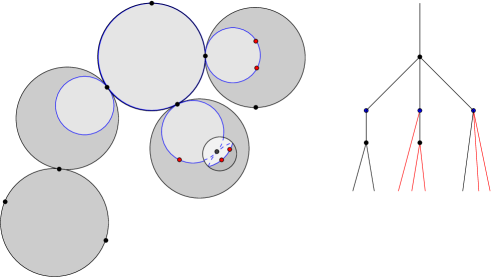
Figure 8. A nodal (3,5)-marked disk

A topology on the moduli space of marked quilted disks can be defined by introducing a suitable notion of convergence. Consider a sequence $(D_{\nu},C_{\nu},\underline{z}_{\nu},\underline{w}_{\nu})$ of marked quilted disks with smooth domain. That is, we assume that $D_{\nu}$ has no nodes so that $D_{\nu}\cong\mathbb{P}^{1}\cong\mathbb{C}\cup\{\infty\}$. For simplicity we may assume that the seam is given by $\operatorname{Im}(z)=\rho_{\nu}$ and the boundary given by $\operatorname{Im}(z)=\epsilon_{\nu}$. Let $(D,C,\underline{z},\underline{w})$ be another marked quilted disk. For $(D_{\nu},C_{\nu},\underline{z}_{\nu},\underline{w}_{\nu})$ to converge to $(D,C,\underline{z},\underline{w})$ we require the following. For each irreducible component $D_{i}$ of $D$ let $\pi_{i}:D\to D_{i}$ denote the unique map that is the identity on $D_{i}$ and constant on all other components. We require a family $\phi_{\nu}:D_{i}\to D_{\nu}$ of holomorphic embeddings (preserving the seams, if $D_{i}$ is quilted) such that for each $k$, either $\phi_{\nu,i}^{-1}(z_{k,\nu})$ converges to $z_{k}$, if $z_{k}$ lies on $D_{i}$, or otherwise to a node $\pi_{i}(z_{k})$ of $D_{i}$; and similarly for each $j$ either $\phi_{\nu,i}^{-1}(w_{j,\nu})$ converges to $w_{j}$ or to a node $\pi_{i}(w_{j})$. The definition of convergence for a fixed combinatorial type is similar, treating each irreducible component separately. In the case of sequences with varying combinatorial type, a subsequence of each fixed type is required to converge to the same limit. We equip $\overline{\mathcal{R}}^{d,e}$ with the topology given by declaring a subset to be closed if it is closed under limits. An argument analogous to [22, 5.6.5] shows that the convergence in the resulting topology is in fact the above notion of convergence. As before in (25), $\overline{\mathcal{R}}^{d,e}$ comes with a universal curve $\overline{\mathcal{U}}^{d,e}$ containing a fiberwise boundary $\partial\mathcal{U}^{d,e}$ as well as a universal seam consisting of isomorphisms classes of tuples $(D,C,\underline{z},\underline{w},y)$ where $y\in C$.

The local structure of these moduli spaces of quilted disks with seam and boundary markings can be described in terms of balanced gluing parameters. Suppose that $\Gamma$ is a combinatorial type of stable $(d,e)$-marked disk. Recall that

$$Z_{\Gamma}\subset\operatorname{Map}(\operatorname{Edge}_{<\infty}(\Gamma),\mathbb{R}_{\geq 0})$$

is the set of balanced gluing parameters from Definition 5.6.

Theorem 6.6 (Existence of compatible tubular neighborhoods for the biassociahedra).

For positive integers $d,e$ and for each combinatorial type $\Gamma$ of $(d,e)$-marked disk, there exist a collection of open neighborhoods $U_{\Gamma}$ of $0$ in $Z_{\Gamma}$ and collar neighborhoods

$$G_{\Gamma}:\mathcal{R}_{\Gamma}^{d,e}\times U_{\Gamma}\to\overline{\mathcal{R}}^{d,e}$$

onto an open neighborhood of $\mathcal{R}^{d,e}_{\Gamma}$ in $\overline{\mathcal{R}}^{d,e}$ that satisfy the following compatibility condition: If $\mathcal{R}^{d,e}_{\Gamma^{\prime}}$ is contained in the closure of $\mathcal{R}^{d,e}_{\Gamma}$ and the local coordinates on $\mathcal{R}^{d,e}_{\Gamma}$ are induced via the gluing construction from those on $\mathcal{R}^{d,e}_{\Gamma^{\prime}}$ then the diagram

$$\begin{diagram}$$

commutes.

Proof.

The proof is a combination of disk gluing and sphere gluing; the former already appeared in the proof of Theorem 5.7. Suppose the following are given:

• a collection of balanced gluing parameters $\delta_{1},\ldots,\delta_{m}$,

• a collection of coordinates $D_{j}-\{w_{j}\}\to\mathcal{H}=\{\operatorname{Im}(z)\geq 0\}$ (for the disk components) so that the seam $C_{j}$ is identified with the set $\{\operatorname{Im}(z)=1\}$; and

• a collection of coordinates $D_{j}-\{w_{j}\}\to\mathbb{C}$ so that the seam $C_{j}$ is $\{\operatorname{Im}(z)=0\}$ (for the quilted sphere components).

Given these data define a glued $(d,e)$-marked disk $G_{\Gamma}(D,\delta)$ by removing small balls around the nodes and gluing small annuli via the relation $z\sim\delta_{j}z$ in the given coordinates, starting recursively with the components furthest away from the root marking $z_{0}$. The seam on the glued component is given by $\{\operatorname{Im}(z)=\delta_{j}\}$. The definition of the seam is independent of $\delta_{j}$ by the balanced condition (42). This construction also works in families: given a family of such coordinates over a stratum $\mathcal{R}^{d,e}_{\Gamma}$, one obtains a collar neighborhood as in the statement of the theorem. Since the space of coordinates on the disks is contractible, we may assume that we have chosen local coordinates so that whenever a point $r\in\mathcal{R}^{d,e}_{\Gamma}$ is in the image of such a gluing map from $\mathcal{R}^{d,e}_{\Gamma^{\prime}}$, the local coordinates are those induced from $\mathcal{R}^{d,e}_{\Gamma^{\prime}}$. ∎

In this sense, the stratified space $\overline{\mathcal{R}}^{d,e}$ is equipped with quilt data as in Definition 2.17: each stratum comes with a collar neighborhood described by gluing parameters compatible with the lower dimensional strata. As with the multiplihedra, the nature of the relations on the gluing parameters only give toric singularities. That is, all corners are polyhedral. The moduli space $\overline{\mathcal{R}}^{2,1}$ is shown in Figure 9.

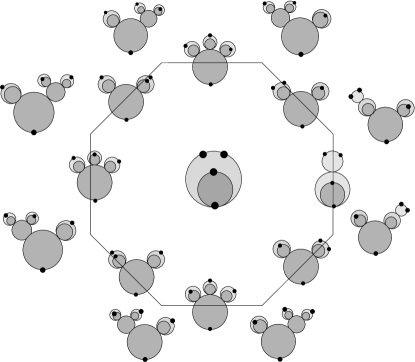
Figure 9. $\overline{\mathcal{R}}^{2,1}$

The moduli space of quilted disks with boundary and seam markings admits natural forgetful maps forgetting both boundary and seam markings generalizing those in (24): For indices $i\in\{1,\ldots,d\}$ and $j\in\{1,\ldots,e\}$ maps (for $d,e\geq 1$)

(55) $$f_{i}:\overline{\mathcal{R}}^{d,e}\to\overline{\mathcal{R}}^{d-1,e},\quad f^{j}:\overline{\mathcal{R}}^{d,e}\to\overline{\mathcal{R}}^{d,e-1}$$

given by forgetting the $i$-th boundary resp. $j$-th seam marking and collapsing unstable components. As in (25), the forgetful morphisms $f_{i}$ may be identified with projection from part of the boundary of the universal curve while the morphism $f^{j}$ may be identified with the part of the universal seam between two markings, with the additional caveat that each nodal point on the seam is potentially replaced with two points as in Figure 10 (so the map to the universal seam is two-to-one in this case.)

Figure 10. The part of the seam between two markings

We leave it to the reader to check that these maps are continuous with respect to the topology on $\overline{\mathcal{R}}^{d,e}$ constructed above and (using the gluing construction) a topological fibration with interval fibers. By induction and the fact that the moduli space $\overline{\mathcal{R}}^{1,0}$ is a point, $\overline{\mathcal{R}}^{d,e}$ is a topological disk. In particular, $\overline{\mathcal{R}}^{d,e}$ is compact and Hausdorff.

Proposition 6.7.

For any positive integers $d,e$, there exists an isomorphism of decomposed spaces from $\overline{\mathcal{R}}^{d,e}$ to $\mathcal{K}^{d,e}$.

Proof.

In the base cases $(d,e)\in\{(1,0),(0,1)\}$ both moduli spaces are points and so the result holds. By the combinatorial description of $\mathcal{K}^{d,e}$ and induction, it suffices to show that the compactified moduli space $\overline{\mathcal{R}}^{d,e}$ is the cone on its boundary. But since $\overline{\mathcal{R}}^{d,e}$ is a topological disk, it is homeomorphic to the cone on its boundary, a sphere. ∎

In order to define the natural transformations, we count quilted surfaces with strip-like ends for a family constructed from the space of quilted disks with interior and exterior markings constructed in the previous section. For analytical reasons, this requires replacing the family of quilted disks in the previous section with one in which degeneration is given by neck-stretching:

Proposition 6.8.

(Existence of families of quilted surfaces with strip-like ends over the bimultiplihedra) For any positive integers $d,e$, there exists a collection of families of quilted surfaces $\overline{\SS}^{d,e}$ with strip-like ends over $\overline{\mathcal{R}}^{d,e}$, with the property that the restriction $\SS^{d,e}_{\Gamma}$ of the family to a stratum $\mathcal{R}_{\Gamma}^{d,e}$ isomorphic to a product of multiplihedra, biassociahedra, and associahedra is a product of the corresponding families of surfaces and quilted surfaces with strip-like ends, and collar neighborhoods of $\SS^{d,e}_{\Gamma}$ are given by gluing along strip-like ends.

Proof.

By induction using Theorem 1.3, starting from the case of three-marked disk where we choose a genus zero surface with strip-like ends, using the already constructed families of surfaces with strip-like ends in Proposition 4.7. ∎

6.2. Natural transformations for cocycles

In this section we construct pseudoholomorphic quilts with interior seam conditions on various Lagrangian correspondences.

Proposition 6.9.

(Existence of families of pseudoholomorphic quilts) Let $M_{0},M_{1}$ be symplectic backgrounds with the same monotonicity constant, $d,e$ positive integers, $\underline{L}^{0},\ldots,\underline{L}^{d}$ admissible generalized Lagrangian branes in $M_{0}$, and $L_{01}^{0},\ldots,L_{01}^{e}$ admissible Lagrangian correspondences from $M_{0}$ to $M_{1}$. For generic choice of perturbation data the moduli spaces of pseudoholomorphic quilts with boundary and seam conditions $(\underline{L}^{i})_{i=0}^{d}$ and $(L_{01}^{j})_{j=0}^{e}$ has

1. finite zero dimensional component $\mathcal{M}^{d,e}_{0}$ and

2. the one-dimensional component $\overline{\mathcal{M}}^{d,e}_{1}$ has boundary equal to the union

   $$\partial\overline{\mathcal{M}}^{d,e}_{1}=\bigcup_{\Gamma}{\mathcal{M}}^{d,e}_{\Gamma,1}$$

   where either (1) $\Gamma$ is stable so that $\mathcal{R}_{\Gamma}^{d,e}$ is a codimension one stratum in $\overline{\mathcal{R}}^{d,0}$ in which case ${\mathcal{M}}^{d,e}_{\Gamma,1}$ is the product of quilted and unquilted components corresponding to the vertices of $\Gamma$, or (2) $\Gamma$ is unstable and corresponds to bubbling off a Floer trajectory.

Proof.

The result follows by applying Theorem 1.4 recursively to the stratified space $\overline{\mathcal{R}}^{d,e}$ constructed in Theorem 6.6. The perturbation over the boundary of $\SS^{d,e}$ is the product of those for the lower-dimensional moduli spaces. ∎

From Theorem 1.5 and the family of quilted surfaces over the moduli space of quilted disks with boundary and seam markings we obtain cochain-level family quilt invariants giving natural transformations:

Definition 6.10.

(Pre-natural transformations for quilted cochains) Let $M_{0},M_{1}$ be symplectic backgrounds with the same monotonicity constant, $d,e$ positive integers, $\underline{L}^{0},\ldots,\underline{L}^{d}$ admissible generalized Lagrangian branes in $M_{0}$, and $L_{01}^{0},\ldots,L_{01}^{e}$ admissible Lagrangian correspondences from $M_{0}$ to $M_{1}$ equipped with widths $\delta^{0},\ldots,\delta^{e}$. To save space in the notation we write $\Phi(L_{01}^{k}):=\Phi(L_{01}^{k},\delta_{0}^{k})$. Given a sequence of homogeneous elements $\alpha_{j}\in CF(L_{01}^{j-1},L_{01}^{j}),j=1,\ldots,e$ define

$$\mathcal{T}^{e}(\alpha_{1},\ldots,\alpha_{e})\in\operatorname{Hom}(\Phi(L_{01}^{0}),\Phi(L_{01}^{e}))$$

as follows: For intersection points $x_{1},\ldots,x_{d}$ of $\underline{L}^{0},\ldots,\underline{L}^{d}$ set

$$(\mathcal{T}^{e}(\alpha_{1},\ldots,\alpha_{e}))^{d}(\langle{x_{1}}\rangle,\ldots,\langle{x_{d}}\rangle)=\Phi_{\SS^{d,e}}(\langle{x_{1}}\rangle,\ldots,\langle{x_{d}}\rangle,\alpha_{1},\ldots,\alpha_{e})(-1)^{\heartsuit+\Box}$$

where $\Box=\sum_{i=1}^{e}i|\alpha_{i}|.$

Theorem 6.11.

(Categorification functor, first version) Let $M_{0},M_{1}$ be symplectic backgrounds with the same monotonicity constant. The maps

$$L_{01}\mapsto\Phi(L_{01}),(\alpha_{1},\ldots,\alpha_{e})\mapsto\mathcal{T}^{e}(\alpha_{1},\ldots,\alpha_{e})$$

define an $A_{\infty}$ functor ${\operatorname{Fuk}}(M_{0}^{-}\times M_{1})\to\operatorname{Func}({\operatorname{Fuk}^{\includegraphics[height=5.05942pt]{sharp.eps}}}(M_{0}),{\operatorname{Fuk}^{\includegraphics[height=5.05942pt]{sharp.eps}}}(M_{1}))$.

Proof.

We show the $A_{\infty}$ functor axiom (78). The axiom follows from a signed count of the boundary components of the one-dimensional component of the moduli space $\mathcal{M}^{d,e}$ in Proposition 6.9. The boundary components are of three combinatorial types:

1. (Quilted sphere bubbles) Facets where some subset of the markings $w_{1},\ldots,w_{e}$ on the interior circle have bubbled off onto a quilted sphere with values in $M_{0},M_{1}$;

2. (Quilted disk bubbles) Facets corresponding to partitions of the interior and exterior markings, corresponding to quilted disk bubbles;

3. (Disk bubbles) Facets where some subset of the markings $z_{1},\ldots,z_{d}$ on the boundary have bubbled off onto a quilted sphere with values in $M_{0}$;

4. (Trajectory bubbling) Bubbling off trajectories at the interior or exterior markings.

See Figure 11 for the case of two interior markings; the facet on the left represents the limit when the two interior marked points come together. Counting boundaries of the first type gives an expression

(56) $$\sum_{i,j}\pm\mathcal{T}^{e-j+1}(\alpha_{1},\ldots,\alpha_{i},\\ \mu^{j}_{{\operatorname{Fuk}}(M_{0}^{-}\times M_{1})}(\alpha_{i+1},\ldots,\alpha_{i+j}),\alpha_{i+j+1},\ldots,\alpha_{e})(\langle{x_{1}}\rangle,\ldots,\langle{x_{d}}\rangle).$$

The second type of boundary component contributes a sum of terms of the form

(57) $$\sum\pm\mu^{m}_{{\operatorname{Fuk}^{\includegraphics[height=5.05942pt]{sharp.eps}}}(M_{1})}(\Phi(L_{01}^{0}))^{i_{1}}(\ldots)\ldots(\Phi(L_{01}^{0}))^{i_{j_{1}-1}}(\ldots)\mathcal{T}^{i_{j_{1}},k_{1}}(\ldots)\\ (\Phi(L_{01}^{1}))^{i_{j_{1}+1}}(\ldots)\ldots(\Phi(L_{01}^{1})^{i_{j_{2}-1}}(\ldots)\mathcal{T}^{i_{j_{2}},k_{2}}(\ldots)\\ \ldots\mathcal{T}^{i_{j_{s}},k_{s}}(\ldots)\Phi(L_{01}^{e})^{i_{j_{s}+1}}(\ldots)\ldots(\Phi(L_{01}^{e})^{i_{m}}(\ldots))$$

where each $\ldots$ is an expression in the $\alpha_{i}$ and $\langle{x_{j}}\rangle$’s, $r$ is the number of bubbles, $s$ is the number of bubbles with interior markings, $i_{l}$ represents the number of exterior markings on the bubbles, $k_{l}$ represents the number of interior markings on bubbles with interior markings, and $j_{1},\ldots,j_{s}$ are the indices of the bubbles with interior markings. The third and fourth type of boundary are similar to those considered before and will not be discussed. Combining this with (82) and (81) proves the $A_{\infty}$ functor axiom up to sign.

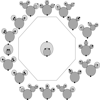
Figure 11. The moduli space $\overline{\mathcal{R}}^{1,2}$

It remains to check the signs. The sign for the inclusion of a facet equal to the image of an embedding $\prod_{i}{\mathcal{R}}^{d_{i},e_{i}}\times{\mathcal{R}}^{f,0}\to\overline{\mathcal{R}}^{d,e}$ is $(-1)^{\sum_{i=1}^{m}(d_{i}-1+e_{i})i+\sum_{i<j}(d_{i}-1)(e_{i})}$. The degree of $\mathcal{T}^{j}(\alpha_{1},\ldots,\alpha_{j})$ is $1-\sum_{i=1}^{j}(1-|\alpha_{i}|).$ The signs appearing in (82) and in the higher compositions are given by sums $\sum_{i<k,j,l}(|x_{i}^{j}|-1)(|y_{k}^{l}|-1)$ where $x_{i}^{j},y_{k}^{l}$ are intersection points corresponding to the inner and outer markings respectively on on the $i$-th resp. $k$-th bubble. The terms of the form $|x_{i}^{j}||y_{k}^{l}|$ are accounted for by Koszul signs. Combining with the two occurrences of $\heartsuit$, this gives the signs claimed in (78). ∎

Remark 6.12.

(Behavior of units under categorification) The functor of Theorem 1.1 is cohomologically unital in the sense that the associated functor

$$H({\operatorname{Fuk}}(M_{0}^{-}\times M_{1}))\to\operatorname{Func}(H{\operatorname{Fuk}^{\includegraphics[height=5.05942pt]{sharp.eps}}}(M_{0}),H{\operatorname{Fuk}^{\includegraphics[height=5.05942pt]{sharp.eps}}}(M_{1}))$$

is unital, by the results of the cohomology level discussion in [42].

To complete the proof of Theorem 1.1, it remains to extend the definition of natural transformations above to the case of generalized Lagrangian correspondences from $M_{0}$ to $M_{1}$:

Remark 6.13.

(Natural transformations for cochains for generalized correspondences) Suppose a sequence of generalized Lagrangian correspondences $\underline{L}_{01}^{j}=L_{01}^{j,1},\ldots,L_{01}^{j,n_{j}}$ of length $n_{j}$ is given. Construct (inductively on the strata) a bundle $\overline{\SS}^{d,e}\to\overline{\mathcal{R}}^{d,e}$ whose fiber at $r\in\overline{\mathcal{R}}^{d,e}$ is a quilted surface with $d$ exterior and $e$ interior quilted strip-like ends, and whose combinatorial type is that of $r$ except that the $j$-th interior segment has been replaced by a collection of strips of length $n_{j}-1$. Counting pairs $(r,\underline{u})$ consisting of a point $r\in\overline{\mathcal{R}}^{d,e}$ together with a pseudoholomorphic quilt $\underline{u}:\overline{\SS}^{d,e}_{r}\to\underline{M}$ with the given Lagrangian boundary and seam conditions defines the natural transformations. The discussion of signs and gradings is similar to that for Theorem 6.11.

As an application of Theorem 1.1, we show that the functors for Lagrangian correspondences constructed in the previous section are independent of all choices up to quasiisomorphism.

Theorem 6.14.

(Independence of the functors up to quasiisomorphism) Let $M_{0},M_{1}$ be symplectic backgrounds with the same monotonicity constant, and let $\underline{L}_{01}$ be an object in ${\operatorname{Fuk}^{\includegraphics[height=5.05942pt]{sharp.eps}}}(M_{0},M_{1})$. The functor $\Phi(L_{01})$ constructed in Section 5 is independent up to quasiisomorphism of all choices (the choice of family of quilts, that is, holomorphic structures on the fibers of $\overline{\SS}^{d,e}\to\overline{\mathcal{R}}^{d,e}$, and the perturbation data.)

Proof.

Suppose two such choices are given, with corresponding functors $\Phi(L_{01}),\Phi^{\prime}(L_{01})$. The Floer cocycle $\alpha\in CF(L_{01},L_{01})$ corresponding to the identity in $HF(L_{01},L_{01})$ defines a natural transformation $\beta$ from $\Phi(L_{01})$ to $\Phi^{\prime}(L_{01})$. Its transpose defines a natural transformation from $\Phi^{\prime}(L_{01})$ to $\Phi(L_{01})$. The composition of the two natural transformations is given by the product of $\alpha$ with $\beta$ under the composition map $\mu^{2}$ in ${\operatorname{Fuk}^{\includegraphics[height=5.05942pt]{sharp.eps}}}(M_{0},M_{1})$. By Theorem 1.1, the composition of natural transformations is the identity transformation. ∎

Proposition 6.15.

(Functor for the diagonal correspondence) Let $M$ be a compact monotone symplectic background. Suppose that $M$ is spin and $\Delta\subset M^{-}\times M$ is the diagonal equipped with the relative spin structure corresponding to a spin structure on $M$. Then $\Phi(\Delta)$ is quasiisomorphic to the identity functor from ${\operatorname{Fuk}^{\includegraphics[height=5.05942pt]{sharp.eps}}}(M)$ to ${\operatorname{Fuk}^{\includegraphics[height=5.05942pt]{sharp.eps}}}(M)$.

Proof.

The correspondence $\Delta$ is quasiisomorphic to $\emptyset$ in ${\operatorname{Fuk}^{\includegraphics[height=5.05942pt]{sharp.eps}}}(M,M)$, with isomorphism given by the cohomological unit in $CF(\Delta)$. By Proposition 5.15 and Theorem 1.1 $\Phi(\Delta)$ is quasiisomorphic to the identity functor in $\operatorname{Func}({\operatorname{Fuk}^{\includegraphics[height=5.05942pt]{sharp.eps}}}(M),{\operatorname{Fuk}^{\includegraphics[height=5.05942pt]{sharp.eps}}}(M))$. ∎

7. Algebraic and geometric composition

In this section we study the composition of $A_{\infty}$ functors for Lagrangian correspondences. In particular, we prove Theorem 1.2 on the homotopy equivalence of the $A_{\infty}$ functor for a geometric composition and the $A_{\infty}$ composition of the corresponding $A_{\infty}$ functors.

7.1. Quilted disks with multiple seams

The proof of the composition result 1.2 depends on generalizations of the multiplihedra which feature multiple interior circles. For $d\geq 1$, let $\mathcal{K}^{d,0,0}$ denote the cell complex whose cells correspond to parenthesized expressions in formal variables $a_{1},\ldots,a_{d}$ and operations $h_{1},h_{2}$ with $h_{2}$ always following $h_{1}$. More precisely, these expressions correspond to bicolored trees which are trees equipped with two types of colored vertices:

Definition 7.1.

(Bicolored trees) A bicolored, rooted tree with $d$ leaves consists of data $(\operatorname{Edge}(\Gamma),\operatorname{Vert}(\Gamma),\operatorname{Edge}_{\infty}(\Gamma),\operatorname{Vert}^{(1)}(\Gamma),\operatorname{Vert}^{(2)}(\Gamma))$ where:

1. (Tree) $\Gamma=(\operatorname{Edge}(\Gamma),\operatorname{Vert}(\Gamma))$ is a tree with vertices $\operatorname{Vert}(\Gamma)$, a collection of (possibly semi-infinite) edges $\operatorname{Edge}(\Gamma)$, and labelling of the semi-infinite edges $\operatorname{Edge}_{\infty}(\Gamma)$ by $\{e_{0},e_{1},\ldots,e_{d}\}$. We call $e_{0}$ the root edge and $e_{1},\ldots,e_{d}$ the leaves.

2. (Colored vertices) There are distinguished subsets $\operatorname{Vert}^{(1)}(\Gamma)\subset\operatorname{Vert}(\Gamma)$ resp. $\operatorname{Vert}^{(2)}(\Gamma)\subset\operatorname{Vert}(\Gamma)$ of vertices of color 1 resp. color 2, such that

   1. any geodesic from a leaf to the root passes through exactly one vertex in $\operatorname{Vert}^{(1)}(\Gamma)$ and exactly one vertex in $\operatorname{Vert}^{(2)}(\Gamma)$;

   2. either $\operatorname{Vert}^{(1)}(\Gamma)=\operatorname{Vert}^{(2)}(\Gamma)$ or $\operatorname{Vert}^{(1)}(\Gamma)\cap\operatorname{Vert}^{(2)}(\Gamma)=\emptyset$;

   3. in the case that $\operatorname{Vert}^{(1)}(\Gamma)\cap\operatorname{Vert}^{(2)}(\Gamma)=\emptyset$, the vertices $\operatorname{Vert}^{(1)}(\Gamma)$ are closer to the root edge.

Such a bicolored tree $\Gamma$ is stable if the valency of every vertex $v\in V$ is 3 or more for $v\notin\operatorname{Vert}^{(1)}\cup\operatorname{Vert}^{(2)}$, and $2$ or more otherwise.

An example of a bicolored tree with one vertex in $\operatorname{Vert}^{(1)}$ shaded darkly and four vertices in $\operatorname{Vert}^{(2)}$ shaded lightly is shown in Figure 12; the remaining vertices are filled.

Figure 12. A stable bicolored tree and the associated algebraic expression

Given such a bicolored tree, the corresponding expression is obtained by using the part of the tree below the second type of colored vertex to determine the parenthesization of the expressions $a_{1},\ldots,a_{d}$, the part of the tree in between the first and colored vertices to determine the parenthesizations of the expressions $h_{2}(\cdot)$, the part of the tree above the first colored vertices to determine the parenthesizations of the expressions $h_{1}(\cdot)$.

A space associated to markings and two operations is constructed inductively from those with fewer markings. For each bicolored tree $\Gamma$ and each vertex $v$ of $\Gamma$, let $\mathcal{K}^{v}$ denote the corresponding associahedron, multiplihedron, or lower dimensional space depending on the valence and whether the vertex is once or twice colored. Define

$$\mathcal{K}_{\Gamma}=\prod_{v\in\operatorname{Vert}(\Gamma)}\mathcal{K}^{v}$$

and $\partial\mathcal{K}^{d,0,0}=\cup_{\Gamma}\mathcal{K}_{\Gamma}/\sim$ where $\sim$ are the equivalences obtained by boundary inclusions. The space is then the cone $\mathcal{K}^{d,0,0}=\operatorname{Cone}(\partial\mathcal{K}^{d,0,0}).$ For example, the cell complex $\mathcal{K}^{2,0,0}$ is a pentagon with vertices labelled by the expressions

$$h_{1}(h_{2}(a_{1})h_{2}(a_{2})),h_{1}(h_{2}(a_{1}))h_{1}(h_{2}(a_{2})),(h_{1}h_{2})(a_{1})(h_{1}h_{2})(a_{2}),h_{1}(h_{2}(a_{1}a_{2})),(h_{1}h_{2})(a_{1}a_{2}).$$

Similar spaces also appear in Batanin [3, end of Section 8] and [4, Example 8.1].

The generalized multiplihedron above has a realization as a moduli space of biquilted disks, described as follows.

Definition 7.2.

(Biquilted disks) For an integer $d\geq 1$ a biquilted disk with $d+1$ markings is a tuple $(D,C_{1},C_{2},z_{0},\ldots,z_{d})$ where

1. $D$ is a holomorphic disk;

2. $(z_{0},\ldots,z_{d})$ is a tuple of distinct points in $\partial D$ whose cyclic order is compatible with the orientation of $\partial D$;

3. $C_{1}$ and $C_{2}$ are nested circles in $D$ with

   $$0<\operatorname{radius}(C_{1})<\operatorname{radius}(C_{2})<\operatorname{radius}(D)$$

   and unique intersection point

   $$C_{1}\cap\partial D=\{z_{0}\}=C_{2}\cap\partial D.$$

An isomorphism of biquilted disks $(D,C_{1},C_{2},z_{0},\ldots,z_{d}),(D^{\prime},C_{1}^{\prime},C_{2}^{\prime},z_{0}^{\prime},\ldots,z_{d}^{\prime})$ is a holomorphic isomorphism of the disks

$$\psi:D\to D^{\prime},\quad\psi(C_{j})=(C_{j}^{\prime}),\ j=1,2,\quad\psi(z_{k})=z_{k}^{\prime},\ k=0,\ldots,d.$$

Let $\mathcal{R}^{d,0,0}$ denote the set of isomorphism classes of biquilted disks with $d+1$ markings.

The moduli space of biquilted disks has a compactification which includes nodal biquilted disks.

Definition 7.3.

(Stable biquilted disks) A nodal biquilted disk with combinatorial type a bicolored tree $\Gamma$ is a collection of unquilted, quilted, and biquilted disks corresponding to the vertices of $\Gamma$ attached at disjoint collections of pairs of points called nodes, together with a collection of markings on the boundary in cyclic order disjoint from the nodes, with the properties that

1. a single inner circle circle appears in the component $D_{v}$ corresponding to $v\in\operatorname{Vert}(\Gamma)$ if and only if $(\operatorname{Vert}^{(1)}(\Gamma)\cap\operatorname{Vert}^{(2)}(\Gamma))=\emptyset$ and $v$ lies in $(\operatorname{Vert}^{(1)}(\Gamma)\cup\operatorname{Vert}^{(2)}(\Gamma))$;

2. exactly two inner circles appear in the component $D_{v}$ corresponding to $v\in\operatorname{Vert}(\Gamma)$ if and only if $v$ lies in $(\operatorname{Vert}^{(1)}(\Gamma)\cap\operatorname{Vert}^{(2)}(\Gamma))$;

3. for any biquilted disk component $D_{v},v\in\operatorname{Vert}^{(2)}(\Gamma)$ the ratio

   $$\operatorname{radius}(C_{2})/\operatorname{radius}(C_{1})\in[1,\infty)$$

   of radii of the two inner circles $C_{1},C_{2}$ is independent of the choice of component

and satisfying the root marking property that the root marking $z_{0}$ is, if it lies on a quilted component, the intersection of the inner circle(s) with the boundary and the monotonicity property that on any non-self-crossing path of components from the root marking $z_{0}$ to the component containing a marking $z_{i}$, there is exactly one component with an inner circle and one component with an outer circle. A nodal biquilted disk is stable if the corresponding bicolored tree is stable, that is, each disk with at least one resp. no interior circles has at least two resp. three special points. Denote by $\overline{\mathcal{R}}^{d,0,0}$ the set of isomorphism classes of stable nodal biquilted disks.

The topology on the moduli space of stable nodal biquilted disks is defined in a similar way as that for the moduli space of stable nodal quilted disks with interior and seam markings in Section 6.1. A sequence of biquilted marked disks is said to converge to a stable limit if, for each component of the limit, there exist a family of reparametrizations satisfying certain properties that we will not detail here. The moduli space $\overline{\mathcal{R}}^{1,0,0}$ is a topological interval while the moduli space $\overline{\mathcal{R}}^{2,0,0}$ is shown in Figure 13.

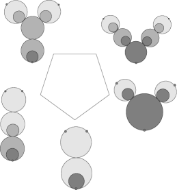
Figure 13. Vertices of $\overline{\mathcal{R}}^{2,0,0}$

The local structure of the moduli space of stable nodal biquilted disks may be described in terms of gluing parameters taking values in the positive real part of a toric variety.

Definition 7.4.

(Balanced gluing parameters) Let

$$\Gamma=(\operatorname{Edge}_{<\infty}(\Gamma),\operatorname{Vert}(\Gamma),\operatorname{Edge}_{\infty}(\Gamma),\operatorname{Vert}^{(1)}(\Gamma),\operatorname{Vert}^{(2)}(\Gamma))$$

be a combinatorial type of a nodal biquilted disk with $d+1$ markings. The set of balanced gluing parameters for $\Gamma$ is the subset $Z_{\Gamma}$ of functions

$$\delta:\operatorname{Edge}_{<\infty}(\Gamma)\to[0,\infty)$$

satisfying the following relations:

• for each $j=1,2$ and for each pair of vertices $v,v^{\prime}$ in $\operatorname{Vert}^{(j)}(\Gamma)$, $\gamma$ the shortest path in $\Gamma$ from $v$ to $v^{\prime}$, the relation

  $$1=\prod_{e\in\gamma}\delta(e)^{\pm 1}$$

  holds as in Definition 5.6.

The various strata are glued together by means of local charts.

Theorem 7.5.

(Existence of Compatible Tubular Neighborhoods) For any integer $d\geq 1$ and any combinatorial type $\Gamma$ of $d+1$-marked biquilted disks there exists a neighborhood $U_{\Gamma}$ of $0$ in $Z_{\Gamma}$ and a collar neighborhood

$$G_{\Gamma}:\mathcal{R}^{d,0,0}_{\Gamma}\times U_{\Gamma}\to\overline{\mathcal{R}}^{d,0,0}$$

of $\mathcal{R}^{d,0,0}_{\Gamma}$ mapping onto onto an open neighborhood of $\mathcal{R}_{\Gamma}^{d,0,0}$ in $\overline{\mathcal{R}}^{d,0,0}$ satisfying the following compatibility property: Suppose that $\mathcal{R}^{d,0,0}_{\Gamma^{\prime}}$ is contained in the closure of $\mathcal{R}^{d,0,0}_{\Gamma}$ and the local coordinates on $\mathcal{R}^{d,0,0}_{\Gamma}$ are induced via the gluing construction from those on $\mathcal{R}^{d,0,0}_{\Gamma^{\prime}}$. Then the diagram

$$\begin{diagram}$$

commutes.

Proof.

The proof uses the same gluing construction as in Theorem 5.7, and is left to the reader. ∎

In this sense, the stratified space of biquilted disks is equipped with quilt data as in Definition 2.17: each stratum comes with a collar neighborhood described by gluing parameters compatible with the lower dimensional strata. As before, there are forgetful morphisms

$$f_{i}:\overline{\mathcal{R}}^{d,0,0}\to\overline{\mathcal{R}}^{d-1,0,0}$$

giving $\overline{\mathcal{R}}^{d,0,0}$ the structure of a topological fibration with interval fibers as in (25). By induction and the fact that $\overline{\mathcal{R}}^{1,0,0}$ is a topological interval, which may be checked explicitly, the space $\overline{\mathcal{R}}^{d,0,0}$ is a topological disk, and in particular a cone on its boundary. By another induction, there is a homeomorphism from $\overline{\mathcal{R}}^{d,0,0}$ to $\mathcal{K}^{d,0,0}$ which respects the combinatorial structure.

Lemma 7.6.

(Ratio of radii map) For any integer $d\geq 1$ there is a continuous map $\rho:\overline{\mathcal{R}}^{d,0,0}\to[0,\infty]$ given on the open stratum by

(58) $$\rho([D,C_{2},C_{1},z_{0},\ldots,z_{d}])=\operatorname{radius}(C_{2})/\operatorname{radius}(C_{1})-1.$$

Proof.

The map $\rho$ is given by the forgetful morphism $\overline{\mathcal{R}}^{d,0,0}\to\overline{\mathcal{R}}^{1,0,0}\cong[0,\infty]$ defined by forgetting all but the $0$-th marking and recursively collapsing unstable components, starting with the components furthest away from the $0$-th marking. ∎

The following description of the boundary of the moduli space of twice-quilted disks is immediate from Definition 7.3:

Proposition 7.7.

(Facets of moduli of biquilted disks) Suppose that a combinatorial type $\Gamma$ of $d$-marked biquilted disks contains $k+1$ vertices with vertices $v_{1},\ldots,v_{k}$ corresponding to biquilted disks, and a vertex $w$ corresponding to an unquilted disk, and corresponds to a facet. Then there exists a homeomorphism

(59) $$\mathcal{R}^{d,0,0}_{\Gamma}\cong(\mathcal{R}^{|v_{1}|,0,0}\times_{[0,\infty]}\ldots\times_{[0,\infty]}\mathcal{R}^{|v_{k}|,0,0}){\times}\mathcal{R}^{|w|}$$

where the fiber product $\mathcal{R}^{v_{1},0,0}\times_{[0,\infty]}\ldots\times_{[0,\infty]}\mathcal{R}^{v_{k},0,0}$ is such that the functions $\rho$ as defined in (58), are all equal on all the components.

Proposition 7.8.

(Classification of facets of the bimultiplihedron) The facets of $\overline{\mathcal{R}}^{d,0,0}\cong\mathcal{K}^{d,0,0}$ are of the following types:

1. (Once-quilted bubbles) a collection of $k$ quilted disks all with seam $C_{2}$ attached to a $k+1$-marked quilted disk with seam $C_{1}$, corresponding to an expression given by

   $$h_{1}(h_{2}(\underline{a}_{1,1}),\ldots,h_{2}(\underline{a}_{1,l_{1}}))\ldots h_{1}(h_{2}(\underline{a}_{i_{r},1}),\ldots,h_{2}(\underline{a}_{i_{r},l_{r}}))$$

   where $\underline{a}_{1,1}\cup\ldots\cup\underline{a}_{i_{r},l_{r}}=(a_{1},\ldots,a_{d})$ is an ordered double partition of the inputs; in which case the facet is the image of an embedding

   $$(\mathcal{K}^{i_{1},0}\times\ldots\times\mathcal{K}^{i_{r},0})\times\mathcal{K}^{r,0}\to\mathcal{K}^{d,0,0}$$

   with $i_{1}+\ldots+i_{r}=d$;

2. (Unquilted bubbles) an unquilted disk attached to a biquilted disk, corresponding to an expression given by

   $$h_{1}h_{2}(a_{1},\ldots,a_{i-1}(a_{i},\ldots,a_{i+j-1}),\ldots,a_{d})$$

   in which case the facet is the image of an embedding

   $$\mathcal{K}^{d_{1}}\times\mathcal{K}^{d_{2},0,0}\to\mathcal{K}^{d_{1}+d_{2},0,0};$$

3. (Biquilted bubbles) a collection of $k$ biquilted disks with seams $C_{1}$ and $C_{2}$ and the same ratio of radii, attached to a single unquilted disk with $k+1$ markings; corresponding to an expression given by

   $$h_{1}h_{2}(a_{1}\ldots a_{i_{1}})\ldots h_{1}h_{2}(a_{d-i_{k}+1},\ldots,a_{d});$$

   in which case the facet is the image of an embedding

   $$\mathcal{K}^{i_{1},0,0}\times_{[0,\infty]}\ldots\times_{[0,\infty]}\mathcal{K}^{i_{k},0,0}\times\mathcal{K}^{j}\mapsto\mathcal{K}^{d,0,0}$$

   for some partition $i_{1}+\ldots+i_{k}=d$;

4. (Seams coming together) a quilted disk with a single seam $C_{1}=C_{2}$, corresponding to the expression $(h_{1}h_{2})(a_{1},\ldots,a_{d})$. In this case the facet is the image of an embedding $\mathcal{K}^{d,0}\to\mathcal{K}^{d,0,0}$.

Proof.

By Theorem 7.5, the codimension of a combinatorial type $\Gamma$ is the number of edges modulo the number of independent relations generated by the balanced condition. Suppose that the root component is not quilted. If there are twice-quilted components, then since the number of independent balanced relations is at least the number of quilted components minus one, and the number of gluing parameters is at least the number of quilted components, no other components besides the root component and twice-quilted components can occur in the codimension one case. If the root component is once-quilted, then the same dimension count implies that all components are once-quilted. Thus codimension one types occur if either there are no nodes and the seams must coincide, a single node, or all nodes must be attached to root component of the configuration. The Proposition follows. ∎

Example 7.9.

The facets of $\overline{\mathcal{R}}^{2,0,0}$ are shown in Figure 14. The five facets are homeomorphic to $\mathcal{R}^{1,0}\times\mathcal{R}^{1,0}\times\mathcal{R}^{2,0},(\mathcal{R}^{1,0,0}\times_{[0,\infty]}\mathcal{R}^{1,0,0})\times\mathcal{R}^{2},\mathcal{R}^{2,0},\mathcal{R}^{2}\times\mathcal{R}^{1,0,0},\mathcal{R}^{2,0}\times\mathcal{R}^{1,0}$ respectively.

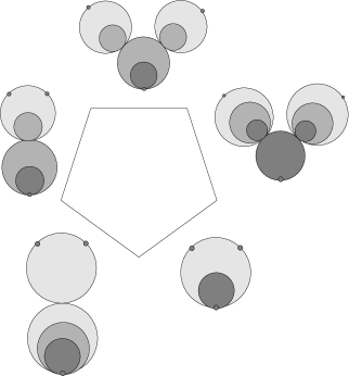
Figure 14. Facets of $\overline{\mathcal{R}}^{2,0,0}$

The moduli space of biquilted disks as cut out of a larger moduli space of free biquilted disks whose definition is obtained by dropping the ratio equality (c) from Definition 7.3, see Figure 15. More precisely,

Definition 7.10.

(Moduli space without relations) Let $\Gamma$ be a combinatorial type of biquilted disk with $k>0$ biquilted disks. Define $\overline{\mathcal{R}}^{{\operatorname{pre}}}_{\Gamma}$ as the product of moduli spaces for the vertices,

$$\overline{\mathcal{R}}_{\Gamma}^{{\operatorname{pre}}}=\prod_{v\in\operatorname{Vert}(\Gamma)}\overline{\mathcal{R}}_{v}.$$

Let

$$\rho_{\Gamma}:\overline{\mathcal{R}}_{\Gamma}^{{\operatorname{pre}}}\to[0,\infty]^{k},\quad r:=(r_{v})_{v\in\operatorname{Vert}(\Gamma)}\mapsto\rho_{\Gamma}(r):=(\rho(r_{v}))_{v\in\operatorname{Vert}^{(1)}(\Gamma)\cap\operatorname{Vert}^{(2)}(\Gamma)}$$

be the map derived from the ratios of the radii of the circles for each biquilted component as in (58), if there are biquilted components, or taking the value $\infty$, if there are no biquilted components.

Figure 15. A free biquilted disk

In terms of the map $\rho_{\Gamma}$ defined in Definition 7.10 we have

(60) $$\overline{\mathcal{R}}_{\Gamma}=\rho_{\Gamma}^{-1}(\Delta)$$

where $\Delta=\{(x,\ldots,x)|x\in\mathbb{R}\}\subset\mathbb{R}^{k}$ is the thin diagonal. The combinatorial type of a free biquilted disk is a free bicolored tree which is defined in the same way as Definition 7.1, but without item (bii). If $\Gamma^{\prime}$ is a combinatorial type of free biquilted disk that is a refinement of $\Gamma$ then the subset $\overline{\mathcal{R}}_{\Gamma}^{{\operatorname{pre}}}\cap\overline{\mathcal{R}}_{\Gamma^{\prime}}^{{\operatorname{pre}}}$ has a neighborhood in $\overline{\mathcal{R}}_{\Gamma}$ given by the gluing construction 7.5.

7.2. Transversality for the ratio map

In this and the following section we define a homotopy between the functor for the geometric composition and the algebraic composition by counting biquilted surfaces with strip-like ends for families of quilted surfaces parametrized by the polytopes $\overline{\mathcal{R}}^{d,0,0}$. Proving transversality of pseudoholomorphic biquilted disks for this family is more delicate than in all the other cases treated previously. This difficulty is due to the fact that in our particular realization of the homotopy multiplihedron as the moduli space $\overline{\mathcal{R}}^{d,0,0}$, some of the boundary strata are fiber products of lower-dimensional strata rather than simply products as in (60).

In order to construct moduli spaces of expected dimension, we allow perturbations in the construction of fiber products. Let $M_{0},M_{1},M_{2}$ be symplectic backgrounds with the same monotonicity constant and $L_{01}\subset M_{0}^{-}\times M_{1}$ and $L_{12}\subset M_{1}^{-}\times M_{2}$ admissible Lagrangian correspondences with brane structures. Let $\underline{L}^{0},\ldots,\underline{L}^{d}$ be admissible generalized Lagrangian branes in $M_{0}$. Given a marked biquilted disk $(D,C_{1},C_{2},z_{0},\ldots,z_{d})$ we label the inner disk resp. middle region resp. outer region by $M_{2}$ resp. $M_{1}$ resp. $M_{0}$, the seams by $L_{01}$ and $L_{12}$, and the components of the outer boundary by $\underline{L}^{0},\ldots,\underline{L}^{d}$. Let $\mathcal{M}^{d,0,0}$ denote the moduli space of biquilted pseudoholomorphic disks, where the surfaces and perturbation data are to be defined inductively.

To carry out the induction we introduce the following notation.

Definition 7.11.

Let $\Gamma$ be a combinatorial type of free biquilted disk with uncolored root vertex $v_{0}$. Denote as follows:

$v_{1},\ldots,v_{k}$	vertices corresponding to outermost quilted or biquilted disk components
$\Gamma_{0}$	smallest subtree of $\Gamma$ containing $v_{0},v_{1},\ldots,v_{k}$
$\gamma_{i}\subset\Gamma_{0}$	non-self-crossing path from $v_{i}$ to the root component $v_{0}$
$|v|$	the valency of $v$
$\mathcal{M}_{v}$	moduli space of pseudoholomorphic quilts $(r,u)$ parametrized by
	$r\in\mathcal{R}^{|v|-1,0,0}$ if $v\in\{v_{1},\ldots,v_{k}\}$ is doubly-quilted
	$r\in\mathcal{R}^{|v|-1,0}$ if $v\in\{v_{1},\ldots,v_{k}\}$ is singly-quilted, and
	$r\in\mathcal{R}^{|v|-1}$ otherwise.

If $k=0$ we take $\Gamma_{0}$ to be the smallest subtree containing all the quilted components.

We suppose that the moduli spaces $\mathcal{M}_{v}$ have been constructed inductively; the actual construction of $\mathcal{M}_{v}$ is carried out in Section 7.3.

Definition 7.12.

(Delay functions etc.) Let $\Gamma$ be a combinatorial type of free biquilted disk with unquilted root component. We think of $[0,\infty]$ as a smooth manifold with boundary, via identification with a finite closed interval. Any element of $\tau\in\mathbb{R}$ defines an automorphism of $[0,\infty]$ fixing $0$ and $\infty$, given by $x\mapsto x{\exp(\tau)}$.

1. (Delay functions) A delay function for $\Gamma$ is a collection of smooth functions depending on $r\in\overline{\mathcal{R}}^{{\operatorname{pre}}}_{\Gamma}$ (see Definition (7.10))

   $$\tau_{\Gamma}=\left(\tau_{e}\in C^{\infty}(\overline{\mathcal{R}}^{{\operatorname{pre}}}_{\Gamma})\right)_{e\in\operatorname{Edge}(\Gamma_{0})}.$$

2. (Delayed evaluation map) Letting $\rho_{i}:=\rho(r_{v_{i}})$ where $\rho$ is the map of (58) taking the ratio of radii of circles, the delayed evaluation map is

   (61) $$\rho_{\tau_{\Gamma}}:\prod\limits_{v\in\operatorname{Vert}(\Gamma)}{\mathcal{M}}_{v} \to [0,\infty]^{k}$$

   $$(r_{v},u_{v})_{v\in\operatorname{Vert}{\Gamma}} \mapsto \left(\rho_{i}\exp\left(\sum_{e\in\gamma_{i}}\tau_{e}(r)\right)\right)_{i=1,\ldots,k}.$$

   That is, the evaluation map is shifted by the sum of delays along each path $\gamma_{i}$ from the root vertex $v_{0}$ to the vertex $v_{i}$ corresponding to a biquilted or outer quilted disk component.

3. (Regular delay functions) Call $\tau_{\Gamma}$ regular if the delayed evaluation map $\rho_{\tau_{\Gamma}}$ is transverse to the diagonal $\triangle\subset(0,\infty)^{k}\subset[0,\infty]^{k}$:

   $$\operatorname{Im}(D_{r,u}\rho_{\tau_{\Gamma}})\oplus T_{\rho_{\tau_{\Gamma}}(r,u)}\triangle=\mathbb{R}^{k},\quad\forall(r,u)\in\prod\limits_{v\in\operatorname{Vert}(\Gamma)}{\mathcal{M}}_{v}.$$

4. (Delayed fiber product) Given a regular delay function $\tau_{\Gamma}$, we define

   (62) $${\mathcal{M}}_{\Gamma}:=\rho_{\tau_{\Gamma}}^{-1}(\triangle).$$

   For a regular delay function $\tau_{\Gamma}$, the delayed fiber product has the structure of a smooth manifold, of local dimension

   (63) $$\dim\mathcal{M}_{\Gamma}=1-k+\sum_{v\in\operatorname{Vert}\Gamma}\dim\mathcal{M}_{v}$$

   where $k$ is the number of biquilted disk components.

The delay functions make the fiber product transverse, so that the zero dimensional moduli spaces behave “as expected”:

Proposition 7.13.

(Only one zero-dimensional bubble for a regular delay function) Let $\Gamma$ be a combinatorial type consisting of a single unquilted disk indexed by a vertex $v\in\operatorname{Vert}\Gamma$ and $k>0$ biquilted disks indexed by vertices $v_{1},\ldots,v_{k}$. If $\tau_{\Gamma}$ is regular, then an isolated point in $\mathcal{M}_{\Gamma}$ consists of an isolated $k$-marked unquilted disk $(r_{v},u_{v})$ in $\mathcal{M}_{v}$, together with a tuple of pseudoholomorphic quilted disks $(r_{v_{i}},\underline{u}_{v_{i}})$ in $\mathcal{M}_{v_{i}},i=1,\ldots,k$, where exactly one of the entries $(r_{v_{j}},\underline{u}_{v_{j}})$ in the tuple comes from a zero-dimensional moduli space $\mathcal{M}_{v_{j}}^{0}$, and the remaining entries $(r_{v_{i}},\underline{u}_{v_{i}}),i\neq j$ come from one-dimensional moduli spaces $\mathcal{M}_{v_{i}}^{1}$.

Proof.

Note the dimension formula (63). The regularity condition on $\tau_{\Gamma}$ implies that $\dim(\mathcal{M}_{v})=0$ and $\dim(\mathcal{M}_{v_{j}})=1$ for all $j$ except for one $j$ for which $\dim(\mathcal{M}_{v_{j}})=0$. ∎

Of course in order to retain compactness the delay functions must be chosen for the strata in a compatible way, detailed below. A delay function for a combinatorial type $\Gamma$ not containing any biquilted disks by convention assigns to any edge the number zero. Let $\tau^{d}=\{\tau_{\Gamma}\}_{\Gamma}$ be a collection of delay functions for each combinatorial type $\Gamma$ of $\partial\overline{\mathcal{R}}^{d,0,0}$. By $\tau_{\Gamma}|\Gamma^{\prime}$ we mean the subset of $\tau_{\Gamma}$ given by edges of $\Gamma^{\prime}$, that is, $\{\tau_{e},e\in\operatorname{Edge}(\Gamma^{\prime})\}$.

Definition 7.14.

(Compatible collections of delay functions) A collection $\{\tau_{\Gamma}\}$ of delay functions is compatible if the following properties hold. Let $\Gamma$ be a combinatorial type of free nodal biquilted disk and $v_{0},\ldots,v_{k}$ as in Definition 7.11.

1. (Subtree property) Let $\Gamma_{1},\ldots,\Gamma_{|v_{0}|-1}$ denote the subtrees of $\Gamma$ attached to $v_{0}$ at its incoming edges; then $\Gamma_{1},\ldots,\Gamma_{|v_{0}|-1}$ are combinatorial types for nodal biquilted disks. Let $r_{i}=(r_{v})_{v\in\operatorname{Vert}(\Gamma_{i})}$ be the components of $r=(r_{v})_{v\in\operatorname{Vert}(\Gamma)}\in\mathcal{R}^{{\operatorname{pre}}}_{\Gamma}$ corresponding to $\Gamma_{i}$. We require that $\tau_{\Gamma}(r)\big{\lvert}_{\Gamma_{i}}=\tau_{\Gamma_{i}}(r_{i}).$ That is, for each edge $e$ of $\Gamma_{i}$, the delay function $\tau_{\Gamma,e}(r)$ is equal to $\tau_{\Gamma_{i},e}(r_{i})$. See Figure 16.

   Figure 16. The (Subtree property)

2. (Infinite or zero ratio property) For each $i$, there exists an open neighborhood of $\rho_{i}^{-1}(0)$ resp. an open neighborhood $\rho_{i}^{-1}(\infty)$ in which all the delays $\tau_{\Gamma,e}$ between the root vertex $v_{0}$ and $v_{i}$ vanish. See Figure 17.

   Figure 17. The (Infinite ratio property)

3. (Refinement property) Suppose that the combinatorial type $\Gamma^{\prime}$ is a refinement of $\Gamma$. That is, suppose there is a surjective morphism $f:\Gamma^{\prime}\to\Gamma$ of trees preserving the labels and mapping colored vertices to colored vertices; let $r$ be the image of $r^{\prime}$ under gluing. Let $U$ be an open neighborhood of $\overline{\mathcal{R}}^{{\operatorname{pre}}}_{\Gamma}$ that is the image of an open neighborhood of $\overline{\mathcal{R}}^{{\operatorname{pre}}}_{\Gamma^{\prime}}$ in $\overline{\mathcal{R}}^{{\operatorname{pre}}}_{\Gamma^{\prime}}\times\mathcal{G}_{\Gamma^{\prime}}$ by the gluing procedure. We require that $\tau_{\Gamma}\big{\lvert}_{U}$ is determined by $\tau_{\Gamma^{\prime}}$ as follows: for each $e\in\operatorname{Edge}(\Gamma)$, and $r\in U$, the delay function for $\Gamma$ is given by

   (64) $$\tau_{\Gamma,e}(r)=\tau_{\Gamma^{\prime},e}+\sum_{e^{\prime}}\tau_{\Gamma^{\prime},e^{\prime}}(r^{\prime})$$

   where the sum is over edges $e^{\prime}$ in $\Gamma^{\prime}$ that are collapsed by $f:\Gamma^{\prime}\to\Gamma$, and the $e$ is the next-furthest-away edge from the root vertex. If $\Gamma^{\prime}$ has no twice-quilted vertices then by the previous item $\tau_{\Gamma}$ vanishes in the gluing region. See Figures 18 and 19.

   Figure 18. The (Refinement property), first case

   In the case that the collapsed edges connect twice quilted components with unquilted components, this means that the delay functions are equal for both types, as in Figure 19.

4. (Core property) Let two combinatorial types $\Gamma$ and $\Gamma^{\prime}$ have the same core $\Gamma_{0}$, let $r,r^{\prime}$ be disks of type $\Gamma$ resp. $\Gamma^{\prime}$ and $r_{0},r^{\prime}_{0}$ the disks of type $\Gamma_{0}$ obtained by removing the components except for those corresponding to vertices of $\Gamma_{0}$. If $r_{0}=r^{\prime}_{0}$ then

   $$\tau_{\Gamma,e}(r)=\tau_{\Gamma^{\prime},e}(r^{\prime}).$$

   That is, the delay functions depend only on the region between the root vertex and the outermost colored vertices.

A collection of compatible delay functions $\{\tau_{\Gamma}\}$ is positive if, for each type $\Gamma$ and every vertex $v\in\Gamma_{0}$ with $k$ incoming edges labeled in counterclockwise order by $e_{1},\ldots,e_{k}$ (that is, the ordering induced by the ordering of the labels on the leaves) their associated delay functions $\tau_{\Gamma,e}$ satisfy $\tau_{\Gamma,e_{1}}<\tau_{\Gamma,e_{2}}<\ldots<\tau_{\Gamma,e_{k}}.$

Figure 19. The (Refinement property), second case

In Figure 19, the second case of the (Refinement property) is illustrated by a situation in which the two nodes labelled $e_{2}$ and $e_{3}$ are resolved, creating a biquilted disk with five unquilted disks attached.

Remark 7.15.

The (Subtree property) allows the inductive construction of delay functions, starting with the strata of lowest dimension, so that the moduli spaces have expected dimension. The (Refinement property) implies that the boundary of the one-dimensional component of the moduli space is the union of moduli spaces for the combinatorial types corresponding to refinements, since the sum (61) matches the sum in (64). The (Core Property) implies that for the types corresponding to bubbling off an unquilted disk is the product of moduli spaces for the components. The (Infinite or Zero Ratio Property) implies that the fiber product is the one expected in the case that there are no biquilted disks.

7.3. Inductive construction of regular, positive, compatible delay functions.

In order to achieve transversality we construct regular, positive delay functions compatibly by induction. The next lemma furnishes the inductive step.

Lemma 7.16.

(Inductive definition of regular positive delay functions) Let $d\geq 1$ be an integer and $\underline{L}=(\underline{L}^{0},\underline{L}^{1},\ldots,\underline{L}^{d},L_{01},L_{12})$ a Lagrangian labeling for biquilted disks with $d+1$ boundary markings. Suppose that for each $1\leq k<d$, the moduli spaces $\mathcal{M}^{k,0,0}(\underline{L}^{\prime})$ have been constructed for all Lagrangian labellings $\underline{L}^{\prime}$ for biquilted disks in $\mathcal{R}^{k,0,0}$ using a compatible, regular, positive collection $\{\tau^{k}(\underline{L}^{\prime})=(\tau_{\Gamma}(\underline{L}^{\prime}))\}_{1\leq k<d}$ of delay functions for less than $d$ leaves. Then there exists an extension of this collection to a regular, compatible, positive collection $\{\tau^{k}(\underline{L})=(\tau_{\Gamma}(\underline{L}))\}_{1\leq k\leq d}$ for at most $d$ leaves.

Proof.

Let $\Gamma$ be a combinatorial type with $d$ incoming markings. We suppose that we have constructed inductively regular delay functions for types $\Gamma^{\prime}$ with $e$ incoming markings for $e<d$, as well as for types $\Gamma^{\prime}$ appearing in the (Refinement property) for $\Gamma$. Note that the case that $\Gamma$ is a maximally-refined combinatorial type, so that the corresponding stratum of the moduli space is zero-dimensional, is covered by the inductive step although in this case there is no “boundary” of the stratum.

We now construct a regular functions $\tau_{\Gamma}:=\tau_{\Gamma}(\underline{L})$. We may assume that $\Gamma$ has no components “beyond the quilted components”. Indeed, by the (Core property) the delay functions are independent of the additional components. (For example, in the case that $\Gamma$ has a single unquilted component as the root, with two nodal points on its boundary, at each of which is attached a biquilted component with a single boundary marking, the moduli space $\overline{\mathcal{R}}^{{\operatorname{pre}}}_{\Gamma}$ is a square, with coordinates given by the ratios between the quilted circles. The inductive hypothesis prescribes the delay functions on the boundary.) The (Subtree property) implies that all the delay functions in $\tau_{\Gamma}:=\tau_{\Gamma}(\underline{L})$ except those for the finite edges adjacent to $v_{0}$, the root component, are already fixed. It remains to find regular delay functions for the finite edges adjacent to the root component of each combinatorial type, in a way that is also compatible with conditions (Infinite or zero ratio property) and (Refinement property). Choose an open neighborhood $U$ of $\partial\overline{\mathcal{R}}^{{\operatorname{pre}}}_{\Gamma}$ in $\overline{\mathcal{R}}^{{\operatorname{pre}}}_{\Gamma}$ in which the delay functions $\tau_{\Gamma}$ for the incoming edges adjacent to the root vertex are already determined by the gluing construction and the delay functions on the boundary. By an argument similar to that of Theorem 3.4 there exists a smaller open neighborhood $V$ of $\partial\mathcal{R}^{{\operatorname{pre}}}_{\Gamma}$ in $\overline{\mathcal{R}}^{{\operatorname{pre}}}_{\Gamma}$ with $\overline{V}\subset U$ such that every element in the zero and one-dimensional components of the $\tau_{\Gamma}$-deformed moduli space $\mathcal{M}_{\Gamma}$ is regular. We show that $\tau_{\Gamma}$ extends over the interior of $\overline{\mathcal{R}}^{{\operatorname{pre}}}_{\Gamma}$. To set up the relevant function spaces let $l\geq 0$ be an integer. Let $C_{\tau_{\Gamma,i}}^{l}(\mathcal{R}^{{\operatorname{pre}}}_{\Gamma})$ denote the Banach manifold of functions with $l$ bounded derivatives on $\mathcal{R}^{{\operatorname{pre}}}_{\Gamma}$, equal to the $i$-th component $\tau_{i}$ of $\tau_{i}$ on $\overline{V}$. Let $\Gamma_{i},i=1,\ldots,n$ be the trees attached to the root vertex $v_{0}$. Consider the evaluation map

$$\operatorname{ev}:\mathcal{M}_{{\Gamma_{1}}}\times\ldots\times\mathcal{M}_{{\Gamma_{n}}}\times\mathcal{M}_{v_{0}}\times\prod_{i=1}^{n}C^{l}_{\tau_{\Gamma,i}}(\mathcal{R}^{{\operatorname{pre}}}_{\Gamma})\to\mathbb{R}^{n-1}$$

$$\left((r_{1},u_{1}),\ldots,(r_{n},u_{n}),(r_{0},u_{0}),\tau_{1},\ldots,\tau_{n}\right)\mapsto$$

$$\left(\rho_{\Gamma_{j}}(r_{j})\exp(\tau_{j}(r))-\rho_{\Gamma_{j+1}}(r_{j+1})\exp(\tau_{j+1}(r))\right)_{j=1}^{n-1}$$

where $r=(r_{0},\ldots,r_{n})$. Note that $0$ is a regular value. The Sard-Smale theorem implies that for $l$ sufficiently large the regular values of the projection

$$\Pi:\operatorname{ev}^{-1}(0)\to\mathcal{T}^{l}(\mathcal{R}^{{\operatorname{pre}}}_{\Gamma}):=\prod_{i=1}^{n}C^{l}_{\tau_{i}}(\mathcal{R}^{{\operatorname{pre}}}_{\Gamma})$$

form a comeager subset. Denote the subset of $\mathcal{T}^{l}(\mathcal{R}^{{\operatorname{pre}}}_{\Gamma})$ consisting of smooth functions by $\mathcal{T}(\mathcal{R}^{{\operatorname{pre}}}_{\Gamma})$.

We use Taubes’ argument (see [22, Section 3.2]) to show that the subset $\mathcal{T}_{{\operatorname{reg}}}(\mathcal{R}^{{\operatorname{pre}}}_{\Gamma})$ of $\mathcal{T}(\mathcal{R}^{{\operatorname{pre}}}_{\Gamma})$ consisting of regular delay functions of class $C^{\infty}$ is dense in $\mathcal{T}(\mathcal{R}^{{\operatorname{pre}}}_{\Gamma})$. (Note here that each of the functions in such a collection extends to the boundary and so defines a function on the closure $\overline{\mathcal{R}}^{{\operatorname{pre}}}_{\Gamma}$.) For each $i=1,\ldots,k$ fix a component of each $\mathcal{M}_{\Gamma_{i}}$ and $\mathcal{M}_{v_{0}}$ of fixed dimension. The product of these components is a connected finite dimensional manifold $X$. Let $K$ be a compact subset of $X$ and let $\mathcal{T}_{{\operatorname{reg}},K}(\mathcal{R}^{{\operatorname{pre}}}_{\Gamma})$ be the subset of smooth delay functions that are regular on $K$. We will show that $\mathcal{T}_{{\operatorname{reg}},K}(\mathcal{R}^{{\operatorname{pre}}}_{\Gamma})$ is open and dense in $\mathcal{T}(\mathcal{R}^{{\operatorname{pre}}}_{\Gamma})$.

To show that $\mathcal{T}_{{\operatorname{reg}},K}(\mathcal{R}^{{\operatorname{pre}}}_{\Gamma})$ is open, we show that the complement is closed. Let $\tau_{\nu}$ be a sequence of smooth delay functions in the complement $\mathcal{T}_{{\operatorname{reg}},K}(\mathcal{R}^{{\operatorname{pre}}}_{\Gamma})^{c}$ converging to a smooth delay function $\tau\in\mathcal{T}(\mathcal{R}^{{\operatorname{pre}}}_{\Gamma})$. Thus we can find a sequence of points $p_{\nu}\in K$ where each $p_{\nu}$ is a critical point of the delayed evaluation map $\rho_{\tau_{\nu}}:X\to\mathbb{R}^{k}$. Passing to a subsequence if necessary, we can assume by the compactness of $K$ that $p_{\nu}\to p\in K$. The delayed evaluation map $\rho_{\tau}:X\to\mathbb{R}^{k}$ for the limit $\tau$ cannot be regular at $p$. Indeed, because if it were regular then for sufficiently large $\nu$ the delay evaluations $\rho_{\tau_{\nu}}$ would be regular at $p_{\nu}$. Hence $p\in K$ is a critical point of $\rho_{\tau}$, and $\tau\in\mathcal{T}_{{\operatorname{reg}},K}(\mathcal{R}^{{\operatorname{pre}}}_{\Gamma})^{c}$. So $\mathcal{T}_{{\operatorname{reg}},K}(\mathcal{R}^{{\operatorname{pre}}}_{\Gamma})^{c}$ is closed in $\mathcal{T}(\mathcal{R}^{{\operatorname{pre}}}_{\Gamma})$. Similarly, let $\mathcal{T}_{{\operatorname{reg}},K}^{l}(\mathcal{R}^{{\operatorname{pre}}}_{\Gamma})$ be the set of $C^{l}$ delay functions that are regular on $K$. By the same argument as above, $\mathcal{T}_{{\operatorname{reg}},K}^{l}(\mathcal{R}^{{\operatorname{pre}}}_{\Gamma})$ is open in $\mathcal{T}^{l}(\mathcal{R}^{{\operatorname{pre}}}_{\Gamma})$. Moreover $\mathcal{T}_{{\operatorname{reg}},K}^{l}(\mathcal{R}^{{\operatorname{pre}}}_{\Gamma})$ is dense in $\mathcal{T}^{l}(\mathcal{R}^{{\operatorname{pre}}}_{\Gamma})$. Indeed $\mathcal{T}_{{\operatorname{reg}},K}^{l}(\mathcal{R}^{{\operatorname{pre}}}_{\Gamma})\supset\mathcal{T}_{{\operatorname{reg}}}^{l}(\mathcal{R}^{{\operatorname{pre}}}_{\Gamma})$ and we already know that $\mathcal{T}_{{\operatorname{reg}}}^{l}(\mathcal{R}^{{\operatorname{pre}}}_{\Gamma})$ is dense in $\mathcal{T}^{l}(\mathcal{R}^{{\operatorname{pre}}}_{\Gamma})$ for sufficiently large $l$.

To show that $\mathcal{T}_{{\operatorname{reg}},K}(\mathcal{R}^{{\operatorname{pre}}}_{\Gamma})$ is dense, fix $\tau\in\mathcal{T}(\mathcal{R}^{{\operatorname{pre}}}_{\Gamma})$. Since $\mathcal{T}^{l}_{{\operatorname{reg}},K}(\mathcal{R}^{{\operatorname{pre}}}_{\Gamma})$ is dense in $\mathcal{T}^{l}(\mathcal{R}^{{\operatorname{pre}}}_{\Gamma})$ we can find

$$\tau_{l}\in\mathcal{T}^{l}_{{\operatorname{reg}},K}(\mathcal{R}^{{\operatorname{pre}}}_{\Gamma}),\quad\|\tau-\tau_{l}\|_{C^{l}}\leq 2^{-l}.$$

Moreover, $\tau_{l}\in\mathcal{T}^{l}_{{\operatorname{reg}},K}(\mathcal{R}^{{\operatorname{pre}}}_{\Gamma})$ is open in $\mathcal{T}^{l}(\mathcal{R}^{{\operatorname{pre}}}_{\Gamma})$. So there exists an $\epsilon_{l}>0$ such that

$$\|\widehat{\tau}-\tau_{l}\|_{C^{l}}<\epsilon_{l}\implies\widehat{\tau}\in\mathcal{T}^{l}_{{\operatorname{reg}},K}(\mathcal{R}^{{\operatorname{pre}}}_{\Gamma}).$$

Since smooth functions are dense in $C^{l}$ this means that we can find

$$\widehat{\tau}_{l}\in\mathcal{T}(\mathcal{R}^{{\operatorname{pre}}}_{\Gamma})\cap\mathcal{T}^{l}_{{\operatorname{reg}},K}(\mathcal{R}^{{\operatorname{pre}}}_{\Gamma}),\quad\|\widehat{\tau}_{l}-\tau_{l}\|_{C^{l}}<\min(\epsilon_{l},2^{-l}).$$

It therefore follows that $\widehat{\tau}_{l}\in\mathcal{T}_{{\operatorname{reg}},K}(\mathcal{R}^{{\operatorname{pre}}}_{\Gamma})$, and $\widehat{\tau}_{l}$ converges as $l\to\infty$ to $\tau$ in the $C^{\infty}$ topology.

Thus $\mathcal{T}_{{\operatorname{reg}},K}(\mathcal{R}^{{\operatorname{pre}}}_{\Gamma})$ is open and dense in $\mathcal{T}(\mathcal{R}^{{\operatorname{pre}}}_{\Gamma})$. We exhaust $X$ with a countable sequence of compact subsets $K$, and there are at most countably many components of each $\mathcal{M}_{\Gamma_{i}}$ and $\mathcal{M}_{v_{0}}$ of a given dimension (i.e. there are countably many $X$). Hence $\mathcal{T}_{{\operatorname{reg}}}(\mathcal{R}^{{\operatorname{pre}}}_{\Gamma})$ is comeager in $\mathcal{T}(\mathcal{R}^{{\operatorname{pre}}}_{\Gamma})$. Finally, the positivity condition is an open condition in $\mathcal{T}(\mathcal{R}^{{\operatorname{pre}}}_{\Gamma})$. So the set of smooth, regular, compatible and positive delay functions is non-empty.

Thus, by induction, there exists a smooth, positive, compatible, regular delay function $\tau_{\Gamma}$ for each combinatorial type of biquilted $d+1$-marked disk, and hence a regular compatible collection $\tau^{d}$.

To apply the induction, note that for $d=1$ the regularity condition is vacuously satisfied (there is no transversality condition to the diagonal) so we may take that as the base step. ∎

7.3.1. Perturbed quilts parametrized by the bimultiplihedron

We now build the family of quilts that will be the domains for our biquilted holomorphic disks. The definition incorporates the inductive procedure for choosing delay functions in the last subsection. The construction here is somewhat different from the constructions in previous chapters in that the families of quilts depend on the choice of Lagrangians.

Definition 7.17.

(Family of quilts parametrized by the bimultiplihedron) Given a positive integer $d$, Lagrangians $\underline{L}=(L_{0},\ldots,L_{d})$, and a delay function $\tau^{d}$, we first define the bundle $\partial\SS^{d,0,0}(\underline{L})\longrightarrow\partial\mathcal{R}^{d,0,0}$ of nodal quilted surfaces with striplike ends over the boundary, $\partial\mathcal{R}^{d,0,0}$. Then we extend it over a neighborhood of the boundary. Finally we choose a smooth interpolation over the remaining interior of $\mathcal{R}^{d,0,0}$. Let

$$\overline{\mathcal{R}}_{\Gamma}^{\tau}:=\rho_{\tau_{\Gamma}}^{-1}(\triangle)\subset\overline{\mathcal{R}}_{\Gamma}^{{\operatorname{pre}}}$$

denote the inverse image of the shifted diagonal as in (62). For different choices of $\tau$ (which are all homotopic) these spaces are isomorphic as decomposed spaces (see Definition 2.12) and so in particular $\overline{\mathcal{R}}_{\Gamma}^{\tau}$ is isomorphic to $\overline{\mathcal{R}}_{\Gamma}$ as a decomposed space. Let

$$\pi_{\Gamma}:\ \overline{\SS}_{\Gamma}^{{\operatorname{pre}}}\to\overline{\mathcal{R}}_{\Gamma}^{{\operatorname{pre}}}$$

denote the product of surface bundles for the vertices of $\Gamma$ already constructed. Let

$$\overline{\SS}_{\Gamma}^{\tau}:=\pi_{\Gamma}^{-1}(\overline{\mathcal{R}}_{\Gamma}^{\tau})$$

denote the restriction to the shifted fiber product. Thus each element of $\overline{\mathcal{M}}_{\Gamma}^{\tau}$ in (62) has domain an element of $\overline{\SS}_{\Gamma}^{\tau}$.

Having defined the family of quilts over the boundary, we extend the bundle over a neighborhood of the boundary. On the facets of $\overline{\mathcal{R}}^{d,0,0}$ for which $\rho\in(0,\infty)$, we use the gluing construction to extend the bundle over a neighborhood of those facets. The codimension one facet where $\rho=0$ does not correspond to the formation of a nodal disk, but rather corresponds to the convergence of the inner and outer seams. Given a family of quilted surfaces over the moduli space of quilted disks with a single seam, we extend the family in a neighborhood of the boundary by replacing the seam by a strip of small width $\rho$ so that is compatible with the gluing construction near its higher codimension boundary strata. For the codimension one facets corresponding to $\rho=\infty$, we take the delay functions to vanish as above in the (Infinite or zero ratio property) and then use the usual gluing construction for the perturbed gluing parameters to extend the bundle over a neighborhood of these boundary strata. Once the bundle is extended over a neighborhood of the boundary we fix a smooth interpolation over the remainder of the interior. This ends the definition.

By Theorem 3.4 we may also extend the regular collection of perturbation data over the boundary $\partial\mathcal{R}^{d,0,0}$ to get regular perturbation data over all of $\overline{\mathcal{R}}^{d,0,0}$. With this data the moduli space $\mathcal{M}^{d,0,0}$ of pseudoholomorphic quilts whose domain is in the family $\SS^{d,0,0,\tau}$, is transversally defined.

Corollary 7.18.

(Description of the ends of the one-dimensional components of the moduli space of biquilted disks) Let $M_{0},M_{1},M_{2}$ be symplectic backgrounds with the same monotonicity constant and

$$L_{01}\subset M_{0}^{-}\times M_{1},\quad L_{12}\subset M_{1}^{-}\times M_{2}$$

admissible Lagrangian correspondences with brane structure. For regular, coherent perturbation data the moduli spaces of pseudoholomorphic quilts ${\mathcal{M}}^{d,0,0}$ have finite zero dimensional component $\mathcal{M}^{d,0,0}_{0}$ and one-dimensional component $\overline{\mathcal{M}}^{d,0,0}_{1}$ that admits a compactification as a one-manifold with boundary the union

(65) $$\partial\overline{\mathcal{M}}^{d,0,0}_{1}=\bigcup_{\Gamma}{\mathcal{M}}^{d,0,0}_{\Gamma,1}$$

where either (1) $\Gamma$ is stable and so $\mathcal{R}_{\Gamma}^{d,0,0}$ is a codimension one stratum in $\overline{\mathcal{R}}^{d,0,0}$, or (2) $\Gamma$ is unstable and corresponds to bubbling off a Floer trajectory.

Proof.

Compactness is by Theorem 3.3. The description (65) of the boundary of the one-dimensional moduli spaces follows from the monotonicity assumptions in Definition 4.4: Any limiting configuration with more than one component has a component with negative index, and so does not exist. ∎

Remark 7.19.

(Orientations for moduli of biquilted disks) The construction of orientations for $\mathcal{M}^{d,0,0}(x_{0},\ldots,x_{d})$ is similar to the previous cases. It depends on a choice of orientation on $\overline{\mathcal{R}}^{d,0,0}$, which itself depends on a choice of slice for the $SL(2,\mathbb{R})$ action on the set of biquilted disks with marking. We take as slice the set of disks with first two marked points fixed and the first inner circle fixed at radius $1/2$. Define a diffeomorphism

$$\mathcal{R}^{d,0,0}\cong\{(z_{2}<\ldots<z_{d},\rho_{2})\}\subset\mathbb{R}^{d}$$

where $\rho_{2}\in(1/2,1)$ is the radius of the second disk. The standard orientation on $\mathbb{R}^{d}$ induces an orientation on $\mathcal{R}^{d,0,0}$.

Figure 20. Desingularization of a biquilted nodal disk

7.4. Homotopy for algebraic composition of correspondences

In this section we compare the composition of $A_{\infty}$ functors for Lagrangian correspondences with the $A_{\infty}$ functor for their algebraic composition. Recall from (17) the definition of algebraic composition: Let

$$L_{01}\subset M_{0}^{-}\times M_{1},\quad L_{12}\subset M_{1}^{-}\times M_{2}$$

be admissible Lagrangian correspondences with brane structure and $\zeta>1$. The algebraic composition of $L_{01},L_{12}$ with width $\zeta$ is the generalized Lagrangian correspondence $L_{01}\includegraphics[height=5.05942pt]{sharp.eps}_{\zeta}L_{12}$ with width $\zeta$ associated to the strips taking values in the manifold $M_{1}$. We compare the functor for the algebraic composition with the composition of functors:

(66) $$\Phi(L_{01}\includegraphics[height=5.05942pt]{sharp.eps}_{\zeta}L_{12}),\ \Phi(L_{12})\circ\Phi(L_{01}):{\operatorname{Fuk}^{\includegraphics[height=5.05942pt]{sharp.eps}}}(M_{0})\to{\operatorname{Fuk}^{\includegraphics[height=5.05942pt]{sharp.eps}}}(M_{2}).$$

Note that these functors act the same way on objects of ${\operatorname{Fuk}^{\includegraphics[height=5.05942pt]{sharp.eps}}}(M_{0})$. The following is a preliminary result towards Theorem 1.2:

Theorem 7.20.

(Algebraic composition theorem) Let $M_{0},M_{1},M_{2}$ be symplectic backgrounds with the same monotonicity constant and $L_{01},L_{12}$ Lagrangian correspondences with admissible brane structures. The $A_{\infty}$ composition $\Phi({L_{12}})\circ\Phi({L_{01}})$ is $A_{\infty}$ homotopic to $\Phi(L_{01}\includegraphics[height=5.05942pt]{sharp.eps}_{\zeta}L_{12})$ in the sense of (83).

Proof.

We suppose that we have constructed smooth moduli spaces of biquilted disks of expected dimension by choosing the perturbation data as in Corollary 7.18. Given admissible generalized Lagrangian branes $\underline{L}^{0},\ldots,\underline{L}^{d}$ for $M_{0}$, define maps

(67) $$\mathcal{H}^{0}_{d}:\operatorname{Hom}(\underline{L}^{0},\underline{L}^{1})\times\ldots\operatorname{Hom}(\underline{L}^{d-1},\underline{L}^{d})\to\operatorname{Hom}(\Phi(L_{01}\includegraphics[height=5.05942pt]{sharp.eps}L_{12})\underline{L}^{0},\Phi(L_{01}\includegraphics[height=5.05942pt]{sharp.eps}_{\zeta}L_{12})\underline{L}^{d})$$

by setting for generalized intersection points $x_{1},\ldots,x_{d}$

(68) $$\mathcal{H}^{0}_{d}(\langle{x_{1}}\rangle,\ldots,\langle{x_{d}}\rangle)=\sum_{u\in\mathcal{M}^{d,0,0}(x_{0},\ldots,x_{d})_{0}}(-1)^{\heartsuit}\epsilon(u)\langle{x_{0}}\rangle$$

where $\epsilon(u)$ are the orientation signs as in (18) and $\heartsuit$ is defined in (28). We write

(69) $$\mathcal{H}^{0,\rho^{\prime}}_{d}=\sum_{\rho^{\prime}}\mathcal{H}^{0,\rho^{\prime}}_{d}$$

where $\mathcal{H}^{0,\rho^{\prime}}_{d}$ is the contribution from biquilted disks $(r,u)$ with (58) $\rho(r)=\rho^{\prime}$. Since the locus of pairs of elements

(70) $$\{(r_{1},u_{1}),(r_{2},u_{2})\in\mathcal{M}^{d_{1},0,0}(x_{0},\ldots,x_{d_{1}})\times\mathcal{M}^{d_{2},0,0}(x_{0},\ldots,x_{d_{2}})\ |\ \rho(r_{1})=\rho(r_{2})\}$$

is negative expected dimension, for generic perturbations the restriction of $\rho$ to the union of the spaces $\mathcal{M}^{d,0,0}(x_{0},\ldots,x_{d})_{0}$ is injective. Similarly, define

$$\mathcal{H}^{1,\rho^{\prime}}_{d}(\langle{x_{1}}\rangle,\ldots,\langle{x_{d}}\rangle)=\sum_{u\in\rho^{-1}(\rho^{\prime})\subset\mathcal{M}^{d,0,0}(x_{0},\ldots,x_{d})_{1}}(-1)^{\heartsuit}\epsilon(u)\langle{x_{0}}\rangle$$

for any $\rho^{\prime}$ such that the intersection in the definition is transverse.

Consider the boundary of the one-dimensional moduli space $\overline{\mathcal{M}}^{d,0,0}(x_{0},\ldots,x_{d})_{1}$. By Corollary 7.18, the boundary points correspond to stable types corresponding to either boundary facets in $\overline{\mathcal{R}}^{d,0,0}$ or bubbled off trajectories. The types of facets are listed in Proposition 7.8. The first type of facet, in which at least two singly-quilted components appear, corresponds to the terms in the definition of the composition of $A_{\infty}$ functors (79). The last type of facet corresponds to the terms in $\Phi({L_{12}\includegraphics[height=5.05942pt]{sharp.eps}L_{01}})$. The remaining boundary components of $\overline{\mathcal{M}}^{d,0,0}(x_{0},\ldots,x_{d})_{1}$ are elements of the strata ${\mathcal{M}}_{\Gamma}^{d,0,0}(x_{0},\ldots,x_{d})_{1}$ where $\Gamma$ is either unstable, corresponding to bubbling off a Floer trajectory, or a stable combinatorial type. The stable combinatorial types are either an unquilted disk mapping to $M_{0}$ and a biquilted disk, or a collection of biquilted disks attached to a unquilted disk mapping to $M_{2}$. Facets corresponding to bubbling off unquilted disks correspond to the last set of terms in the definition of homotopy of $A_{\infty}$ functors in (81) with the homotopy $\mathcal{T}^{d}=\mathcal{H}^{0}_{d}$ defined in (67). It remains to show that facets representing bubbling off quilted disks correspond to the first set of terms in (81). On the $m$ biquilted disks we have $m-1$ relations, requiring that the inner/outer ratios be equal up to the shifts $\tau_{\Gamma}$. By Proposition 7.13, for $m-1$ of the bubbles, the unconstrained moduli space is dimension $1$, and exactly for one of the bubbles, say the $i$-th, the unconstrained moduli space is dimension $0$. Thus the contribution of this type of facet is

(71) $$\sum_{\rho,I_{1},\ldots,I_{r},i}\mu^{m}_{{\operatorname{Fuk}^{\includegraphics[height=5.05942pt]{sharp.eps}}}(M_{2})}(\mathcal{H}^{1,\rho+\tau_{\Gamma,1}}(\langle{x_{I_{1}}}\rangle),\ldots,\mathcal{H}^{1,\rho+\tau_{\Gamma,i-1}}(\langle{x_{I_{i-1}}}\rangle),\mathcal{H}^{0,\rho+\tau_{\Gamma,i}}(\langle{x_{I_{i}}}\rangle),\\ \mathcal{H}^{1,\rho+\tau_{\Gamma,i+1}}(\langle{x_{I_{i+1}}}\rangle),\ldots,\mathcal{H}^{r,\rho+\tau_{\Gamma,r}}(\langle{x_{I_{r}})}\rangle)$$

where

$$\mathcal{H}^{1,\rho_{0}}_{d}(\langle{x_{1}}\rangle,\ldots,\langle{x_{d}}\rangle)=\sum_{u\in\mathcal{M}^{d,0,0}({x_{0}},\ldots,{x_{d}})_{1},\rho(u)=\rho_{0}}(-1)^{\heartsuit}\epsilon(u)\langle{x_{0}}\rangle$$

counts over the moduli space of expected dimension one, of fixed ratio $\rho_{0}$.

In order to define a homotopy between $\Phi(L_{12})\circ\Phi(L_{01})$ and $\Phi(L_{01}\includegraphics[height=5.05942pt]{sharp.eps}_{\zeta}L_{12})$, we “integrate over $\rho$” in the following sense. First we consider the case that there are finitely many contributions to $\mathcal{H}^{0}$. Since the restriction of $\rho$ to the zero-dimensional component of the moduli space is injective, see the discussion after (70), we may divide $(0,\infty)$ into finitely many intervals $[a_{i},a_{i+1}],i=0,\ldots,s$ such that there is at most one contribution to $\mathcal{H}^{0}$ in each interval occurring at say $\rho^{-1}(\delta_{i})$. The intersections $\mathcal{M}^{d,0,0}(x_{1},\ldots,x_{d})_{1}\cap\rho^{-1}(a_{i})$ and $\mathcal{M}^{d,0,0}(x_{1},\ldots,x_{d})_{1}\cap\rho^{-1}(a_{i+1})$ are components in the boundary of $\mathcal{M}^{d,0,0}(x_{1},\ldots,x_{d})_{1}\cap\rho^{-1}([a_{i},a_{i+1}])$. The other boundary components correspond to bubbling off unquilted disks from a twice-quilted disk, or bubbling off a number of quilted disks. Thus

(72) $$\mathcal{H}^{1,a_{i+1}}(\langle{x_{1}}\rangle,\ldots,\langle{x_{d}}\rangle)=\mathcal{H}^{1,a_{i}}(\langle{x_{1}}\rangle,\ldots,\langle{x_{d}}\rangle)+\\ \pm\sum_{I_{1},\ldots,I_{r}}\mu^{m}_{{\operatorname{Fuk}^{\includegraphics[height=5.05942pt]{sharp.eps}}}(M_{2})}(\mathcal{H}^{n_{1},\delta+\tau_{\Gamma,1}}(\langle{x_{I_{1}}}\rangle),\ldots,\mathcal{H}^{n_{m},\delta+\tau_{\Gamma,m}}(\langle{x_{I_{m}}}\rangle))\\ \pm\sum_{\delta_{i},j,k}\mathcal{H}^{0,\delta}(\langle{x_{1}}\rangle,\ldots,\mu^{k}_{{\operatorname{Fuk}^{\includegraphics[height=5.05942pt]{sharp.eps}}}(M_{0})}(\langle{x_{j+1}}\rangle,\ldots,\langle{x_{j+k}}\rangle),\langle{x_{j+k+1}}\rangle,\ldots,\langle{x_{d}}\rangle).$$

where each $n_{l}\in\{0,1\}$ and $\sum_{i=1}^{m}(n_{i}-1)=-1$, by the transversality assumption. For each $u\in\mathcal{H}^{0,\delta_{i}}(\cdot)$, we have $n_{k(u)}=0$ for some $k(u)$ and otherwise $n_{l}=1,l\neq k(u)$, see Proposition 7.13. Now by assumption, there are no other values of the restriction of $\rho$ to $\mathcal{M}^{l,0,0}(\cdot)_{0},l\leq d$ in $[a_{i},a_{i+1}]$. It follows that the moduli spaces $\mathcal{M}^{|I_{j}|,0,0}(x_{I_{j}})_{1}\cap\rho^{-1}([a_{i},\delta])$ have boundary given by

(73) $$\partial\mathcal{M}^{|I_{j}|,0,0}(x_{I_{j}})_{1}\cap\rho^{-1}([a_{i},\delta])=\mathcal{M}^{|I_{j}|,0,0}(x_{I_{j}})_{1}\cap\rho^{-1}(\{a_{i},\delta\}),j<k(u)$$

$$\partial\mathcal{M}^{|I_{j}|,0,0}(x_{I_{j}})_{1}\cap\rho^{-1}([\delta,a_{i+1}])=\mathcal{M}^{|I_{j}|,0,0}(x_{I_{j}})_{1}\cap\rho^{-1}(\{\delta,a_{i+1}\}),j>k(u).$$

Since the delay functions are positive by assumption, these equalities hold after replacing $\delta$ with the nearby values $a_{i},a_{i+1}$:

(74) $$\mathcal{H}^{1,\delta}(\langle{x_{I_{j}}}\rangle)=\mathcal{H}^{1,a_{i}}(\langle{x_{I_{j}}}\rangle),\quad j<k(u),\quad\mathcal{H}^{1,\delta}(\langle{x_{I_{j}}}\rangle)=\mathcal{H}^{1,a_{i+1}}(\langle{x_{I_{j}}}\rangle),\quad j>k(u).$$

By substituting these equalities into (72), we obtain the terms in the definition of $A_{\infty}$ homotopy between the functors with ratio $a_{i}$ and those for ratio $a_{i+1}$. Taking the composition of these homotopies as in (84) proves the theorem for $\rho>0$, up to sign in the case that the number of contributions to $\mathcal{H}^{0}$ is finite.

In general we define the homotopy by an inductive limit. For each $d_{0}$ there are finitely many contributions to $\mathcal{H}^{0,d}$ for $d\leq d_{0}$. The construction of the previous paragraph yields a map

$$\mathcal{T}^{\leq d}=\mathcal{H}^{0,\delta_{1}}\circ(\mathcal{H}^{0,\delta_{2}}\circ(\ldots\circ\mathcal{H}^{0,\delta_{s}})\ldots)$$

that is a homotopy of $A_{\infty}$ functors from $\Phi(L_{12})\circ\Phi(L_{01})$ to $\Phi(L_{01}\includegraphics[height=5.05942pt]{sharp.eps}_{\zeta}L_{12})$ up to terms involving composition maps involving more than $d$ entries. That is, the collections

$$(\Phi(L_{12})\circ\Phi(L_{01}))_{d\leq d_{0}},\quad(\Phi(L_{01}\includegraphics[height=5.05942pt]{sharp.eps}L_{12}))_{d\leq d_{0}},\quad(\mathcal{H}^{0,n})_{d\leq d_{0}}$$

satisfy equation (81) for $d\leq d_{0}$. Furthermore by construction if $d<e$ then $\mathcal{T}^{\leq d,i}=\mathcal{T}^{\leq e,i}$ for $i\leq d$, since the higher corrections only involve maps with high numbers of inputs. It follows that the limit

$$\mathcal{T}:=\lim_{d_{0}\to\infty}\mathcal{T}^{\leq d_{0}}$$

is well-defined. Furthermore the “differential” of $\mathcal{T}$ is the limit

$$(\mu^{1}_{\operatorname{Hom}(\mathcal{F}_{1},\mathcal{F}_{2})}\mathcal{T})^{d}=\lim_{d_{0}\to\infty}(\mu^{1}_{\operatorname{Hom}(\mathcal{F}_{1},\mathcal{F}_{2})}\mathcal{T}^{\leq d_{0}})^{d}.$$

So $\mathcal{T}=(\mathcal{T}^{d})_{d\geq 0}$ is a homotopy from $\Phi(L_{12})\circ\Phi(L_{01})$ to $\Phi(L_{01}\includegraphics[height=5.05942pt]{sharp.eps}_{\zeta}L_{12})$.

It remains to check the signs. Since $|\mathcal{T}|=|\mathcal{H}|=-1$, the signs in the formula (83) vanish. Consider the signs of the inclusions of strata into $\overline{\mathcal{R}}^{d,0,0}$: An embedding $\mathcal{R}^{f}\times\mathcal{R}^{e,0,0}\to\overline{\mathcal{R}}^{d,0,0}$ corresponding to an unquilted bubble containing the markings $i+1,\ldots,i+f$ has sign $(-1)^{if+i}$, cf. (32). For the facets induced by embeddings $(\mathcal{R}^{i_{1},0}\times\ldots\times\mathcal{R}^{i_{m},0})\times\mathcal{R}^{e,0}\to\overline{\mathcal{R}}^{d,0,0}$ gluing acts on signs by $1+(-1)^{\sum_{j=1}^{m}(m-j)(i_{j}-1)}$ c.f. Lemma 5.9. For the facets induced by embeddings $(\mathcal{R}^{i_{1},0,0}\times_{[0,\infty]}\ldots\times_{[0,\infty]}\mathcal{R}^{i_{m},0,0})\times\mathcal{R}^{m}\to\overline{\mathcal{R}}^{d,0,0}$ (where the real number is the ratio of the radii of the two interior circles) the gluing map has sign $1+(-1)^{\sum_{j=1}^{m}(m-j)i_{j}}$. For the facet given by the embedding $\mathcal{R}^{d,0}\to\overline{\mathcal{R}}^{d,0,0}$ the gluing map is orientation preserving. The signs for the embeddings of the facets combine with the Koszul signs to give the signs in the formulas (83) and (81). ∎

7.5. Homotopy for geometric composition of correspondences

In this section we prove Theorem 1.2 relating the composition of functors with the functor for the composition of correspondences. First we show that the $A_{\infty}$ functors are quasi-isomorphic. Let $L_{01},L_{12}$ be Lagrangian correspondences as above with the property that the geometric composition $L_{02}:=L_{01}\circ L_{12}$ is smooth and embedded by projection into $M_{0}^{-}\times M_{2}$ as in (1).

Proposition 7.21.

(Algebraic versus geometric composition) Let $M_{0},M_{1},M_{2}$ be symplectic backgrounds with the same monotonicity constant and $L_{01}\subset M_{0}^{-}\times M_{1}$ and $L_{12}\subset M_{1}^{-}\times M_{2}$ admissible Lagrangian correspondences with brane structure. Suppose that $L_{02}=L_{01}\circ L_{12}$ is transverse and embedded, and admissible in $M_{0}^{-}\times M_{2}$. Then for any $\zeta>0$ the functors $\Phi(L_{01}\includegraphics[height=5.05942pt]{sharp.eps}_{\zeta}L_{12})$ and $\Phi(L_{02})$ are quasi-isomorphic in $\operatorname{Func}({\operatorname{Fuk}^{\includegraphics[height=5.05942pt]{sharp.eps}}}(M_{0}),{\operatorname{Fuk}^{\includegraphics[height=5.05942pt]{sharp.eps}}}(M_{2}))$.

Proof.

Theorem 7.20 shows that $\Phi(L_{12})\circ\Phi(L_{01})$, $\Phi(L_{01}\includegraphics[height=5.05942pt]{sharp.eps}_{\zeta}L_{12})$ are homotopic, in particular, quasiisomorphic. To show that $\Phi(L_{01}\includegraphics[height=5.05942pt]{sharp.eps}_{\zeta}L_{12}),\Phi(L_{02})$ are quasi-isomorphic recall that in [42] the second two authors constructed cocycles $\phi\in CF(L_{01}\includegraphics[height=5.05942pt]{sharp.eps}_{\zeta}L_{12},L_{02})$ and $\psi\in CF(L_{02},L_{01}\includegraphics[height=5.05942pt]{sharp.eps}_{\zeta}L_{12})$ with the property that

(75) $$[\psi]\circ[\phi]=1_{L_{02}}\in HF(L_{02},L_{02}),\quad[\psi]\circ[\phi]=1_{L_{01}\includegraphics[height=5.05942pt]{sharp.eps}_{\zeta}L_{12}}\in HF(L_{01}\includegraphics[height=5.05942pt]{sharp.eps}L_{12},L_{01}\includegraphics[height=5.05942pt]{sharp.eps}_{\zeta}L_{12}).$$

An alternative argument for the existence of the cocycle is given in Lekili-Lipyanskiy [18]. Let $T(\phi),T(\psi)$ denote the corresponding natural natural transformations. It follows from (75) that

$$T(\phi)\circ T(\psi)\in\operatorname{Aut}(\Phi(L_{01}\includegraphics[height=5.05942pt]{sharp.eps}_{\zeta}L_{12})),\quad T(\psi)\circ T(\phi)\in\operatorname{Aut}(\Phi(L_{02}))$$

are cohomologous to the identity natural transformations. The proposition follows by combining (75), Theorem 1.1, and Theorem 7.20. ∎

Proof of Theorem 1.2.

The statement of the Theorem is a parametrized version of the main result of [43]. We construct a family of quilted surfaces $\overline{\SS}^{d,0,0}$ over the bimultiplihedron $\overline{\mathcal{R}}^{d,0,0}$ for which the strip with boundary conditions $L_{01},L_{12}$ has varying width between $0$ and $\infty$; this differs from the algebraic composition theorem where the width was bounded below by a non-zero constant $\rho_{0}$. Such a family can be obtained from $\overline{\SS}^{d,0}$ by inserting a strip of width $\zeta$ for $\zeta$ small and varying, and extended to a family $\overline{\SS}^{d,0,0}$ over $\overline{\mathcal{R}}^{d,0,0}$ by the previous procedure. The argument will be the same as that for the algebraic composition in Theorem 7.20, but the facet of $\overline{\mathcal{R}}^{d,0,0}$ where the seams come together has fibers given by quilted disks with a single seam. The corresponding boundary stratum in the moduli space of pseudoholomorphic quilts now corresponds to the terms for the geometric composition $\Phi(L_{01}\circ L_{12})$ in the statement of Theorem 1.2.

To show that the moduli space of pseudoholomorphic quilts over this new family has the same properties as before requires the arguments of [43]: Near any pseudoholomorphic quilt with seam in $L_{02}$ there is a unique nearby pseudoholomorphic quilt with small width $\zeta$ of the strip in between the seams labelled $L_{01}$ and $L_{12}$, by a parametrized version of the implicit function theorem given in [43]. The operation of replacing the seam with a strip of width $\zeta$ defines a thickening map

$$T_{r}:\mathcal{R}^{d,0}\times[0,\delta)\to\overline{\mathcal{R}}^{d,0,0}.$$

Given a quilt $\underline{u}:\underline{S}\to\underline{M}$ with seam $I$ mapping to $L_{02}$, we denote by $\underline{S}(\zeta)$ the quilt obtained by replacing the seam $I$ with a strip $S_{\zeta}=\mathbb{R}\times[0,\zeta]$. Let $\gamma:I\to L_{01}\times_{M_{1}}L_{12}$ be the unique lift of the restriction of $\underline{u}$ to $I$. Let $\underline{u}(\zeta):\underline{S}(\zeta)\to\underline{M}$ be the map equal to $\underline{u}$ on the components except $S_{\zeta}$, and $\underline{u}(\zeta)(s,t)=\pi_{1}(\gamma(s))$ on $S_{\zeta}$. Given a section $\underline{\xi}$ of $\underline{u}(\zeta)^{*}T\underline{M}$ with Lagrangian boundary and seam conditions, a suitable exponential $e_{\underline{u}}(\underline{\xi}):\underline{S}\to\underline{M}$ with the Lagrangian boundary and seam conditions is defined in [43, 20]. Pseudoholomorphic quilts near $\underline{u}$ correspond to pairs $r^{\prime}\in\SS^{d,0,0},\underline{v}:\underline{S}_{r}\to\underline{M}$ with $r^{\prime}=T_{r}(\sigma,\zeta),\quad\underline{v}=e_{\underline{u}}(\underline{\xi})$. These are zeroes of the map

(76) $$\mathcal{F}_{\underline{u},\zeta}:T_{r}\mathcal{R}^{d,0}\times\Omega^{0}(\underline{S}_{T_{r}(\sigma,\zeta)}^{d,0},\underline{u}(\zeta)^{*}T\underline{M})\to\Omega^{0,1}(\underline{S}_{T_{r}(\sigma,\zeta)}^{d,0},\underline{u}(\zeta)^{*}T\underline{M}),\\ (\sigma,\underline{\xi})\mapsto\Phi_{\underline{u}(\zeta)}^{-1}\overline{\partial}_{T_{r}(\sigma,\zeta),\underline{J},\underline{K}}e_{\underline{u}}(\underline{\xi})$$

where $\Phi_{\underline{u}(\zeta)}^{-1}$ denotes almost complex parallel transport. In a suitable Sobolev completion, the map $\mathcal{F}_{\underline{u},\zeta}$ is Fredholm and satisfies uniform quadratic and error estimates, and has a derivative with uniformly bounded right inverse. As in [43] the argument requires splitting off two more strips of width $\zeta$ near the seam, and using the folding construction in [43, Section 3]. The Sobolev completions are described in [43, Section 3.1], the difference here being the presence of additional $T_{r}\mathcal{R}^{d,0}$ in the map. This change does not affect any of the estimates: the variation of the complex structure on the once-quilted strip does not affect the complex structure of the corresponding biquilted strips near the seam. It follows that the additional terms as in [21] are independent of $\zeta$. To show compactness of the resulting moduli spaces, the argument of [43, Section 3.3] shows that, due to the monotonicity assumptions, disk, sphere, and figure eight bubbles cannot occur in the limit $\zeta\to 0$. Indeed, by energy quantization such bubbles can only occur at finitely many points, for any sequence of pseudoholomorphic quilts of index one or zero. By removal of singularities one obtains in the limit on the complement of the bubbling set a configuration with lower energy, hence index. Such a configuration cannot occur by the regularity hypotheses. ∎

The following simple case of Theorem 1.2 gives independence of the Fukaya category from all choices:

Corollary 7.22.

(Independence of the Fukaya category from choices up to homotopy equivalence) Let $M$ be a symplectic background. The Fukaya category ${\operatorname{Fuk}}(M)$ and generalized Fukaya category ${\operatorname{Fuk}^{\includegraphics[height=5.05942pt]{sharp.eps}}}(M)$ are independent of all choices used to construct it, up to $A_{\infty}$ homotopy equivalence.

Proof.

Let ${\operatorname{Fuk}}(M)^{0},{\operatorname{Fuk}}(M)^{1}$ denote the Fukaya categories defined using two different sets of perturbation data. The empty generalized correspondence gives functors $\Phi(\emptyset)^{01}:{\operatorname{Fuk}}(M)^{0}\to{\operatorname{Fuk}}(M)^{1}$ and vice versa, for different choices of data. For the same choice of data the empty correspondence gives the identity functor by Proposition 5.15. Since the composition of two empty correspondences is empty, we obtain from Theorem 1.2 an $A_{\infty}$ homotopy between $\Phi(\emptyset)^{01}\circ\Phi(\emptyset)^{10}$ and the identity, and similarly for $\Phi(\emptyset)^{10}\circ\Phi(\emptyset)^{01}$. ∎

8. Conventions on $A_{\infty}$ categories

The machinery of $A_{\infty}$ (homotopy associative) algebras was introduced by Stasheff [33] as a way of recognizing chains on loop spaces. Later Fukaya [10] introduced $A_{\infty}$ categories as a way of understanding product structures in Lagrangian Floer cohomology. In this appendix we describe our conventions for $A_{\infty}$ categories, which attempt to follow those of Seidel [29]. Other references for this material are Fukaya [9], Lefévre-Hasegawa [17], and Lyubashenko [19]. Kontsevich-Soibelman [15] introduce a more conceptual framework in which $A_{\infty}$ algebras are non-commutative formal pointed differential-graded manifolds; in particular this approach gives a conceptual framework for the signs in the definitions below. Let $N\in 2\mathbb{N}\cup\{\infty\}$ be an even positive integer, or infinity. In the case $N=\infty$, we adopt the convention $\mathbb{Z}_{N}=\mathbb{Z}$.

Definition 8.1.

($A_{\infty}$ categories, functors etc.)

1. ($A_{\infty}$ categories) A $\mathbb{Z}_{N}$-graded $A_{\infty}$ category $\mathcal{C}$ consists of the following data:

   1. A class of objects $\operatorname{Obj}(\mathcal{C})$;

   2. for each pair $C_{1},C_{2}\in\operatorname{Obj}(\mathcal{C})$, a $\mathbb{Z}_{N}$-graded abelian group of morphisms $\operatorname{Hom}_{\mathcal{C}}(C_{1},C_{2})=\bigoplus_{i\in\mathbb{Z}_{N}}\operatorname{Hom}_{\mathcal{C}}^{i}(C_{1},C_{2});$

   3. for each $d\geq 0$ and $(d+1)$-tuple $C_{0},\ldots,C_{d}\in\operatorname{Obj}(\mathcal{C})$, a multilinear composition map

      $$\mu^{d}_{\mathcal{C}}:=\mu^{d}_{\mathcal{C},C_{0},\ldots,C_{d}}:\ \operatorname{Hom}_{\mathcal{C}}(C_{0},C_{1})\otimes\ldots\otimes\operatorname{Hom}_{\mathcal{C}}(C_{d-1},C_{d})\to\operatorname{Hom}_{\mathcal{C}}(C_{0},C_{d})[2-d]$$

   satisfying the $A_{\infty}$ -associativity equations

   (77) $$0=\sum_{n+m\leq d}(-1)^{n+\sum_{i=1}^{n}|a_{i}|}\mu_{\mathcal{C}}^{d-m+1}(a_{1},\ldots,a_{n},\\ \mu_{\mathcal{C}}^{m}(a_{n+1},\ldots,a_{n+m}),a_{n+m+1},\ldots,a_{d})$$

   for any tuple of homogeneous elements $a_{1},\ldots,a_{d}$. The signs are the shifted Koszul signs, that is, the Koszul signs for the shifted grading in which the structure maps have degree one as in Kontsevich-Soibelman [15]. The element $\mu_{\mathcal{C},C_{0}}^{0}(1)\in\operatorname{Hom}(C_{0},C_{0})[2]$ is the curvature of the object $C_{0}$. An $A_{\infty}$ category is flat if $\mu_{\mathcal{C},C_{0}}^{0}(1)$ vanishes for every object $C_{0}$. We remark that we do not assume that our $A_{\infty}$ categories have units.

2. ($A_{\infty}$ functor) Let $\mathcal{C}_{0},\mathcal{C}_{1}$ be flat $A_{\infty}$ categories. An $A_{\infty}$ functor $\mathcal{F}$ from $\mathcal{C}_{0}$ to $\mathcal{C}_{1}$ consists of the following data:

   1. a map $\mathcal{F}:\operatorname{Obj}(\mathcal{C}_{0})\to\operatorname{Obj}(\mathcal{C}_{1})$; and

   2. for any $d\geq 1$ and $d+1$-tuple $C_{0},\ldots,C_{d}\in\operatorname{Obj}(\mathcal{C}_{0})$, a map

      $$\mathcal{F}^{d}:\ \operatorname{Hom}(C_{0},C_{1})\times\ldots\operatorname{Hom}(C_{d-1},C_{d})\to\operatorname{Hom}(\mathcal{F}(C_{0}),\mathcal{F}(C_{d}))[1-d]$$

   such that the following holds:

   (78) $$\sum_{i+j\leq d}(-1)^{i+\sum_{j=1}^{i}|a_{j}|}\mathcal{F}^{d-j+1}(a_{1},\ldots,a_{i},\mu_{\mathcal{C}_{0}}^{j}(a_{i+1},\ldots,a_{i+j}),a_{i+j+1},\ldots,a_{d})=\\ \sum_{m\geq 1}\sum_{i_{1}+\ldots+i_{m}=d}\mu_{\mathcal{C}_{1}}^{m}(\mathcal{F}^{i_{1}}(a_{1},\ldots,a_{i_{1}}),\ldots,\mathcal{F}^{i_{m}}(a_{i_{1}+\ldots+i_{m-1}+1},\ldots,a_{d})).$$

3. (Composition of $A_{\infty}$ functors) The composition of $A_{\infty}$ functors $\mathcal{F}_{1},\mathcal{F}_{2}$ is defined by composition of maps on the level of objects, and

   (79) $$(\mathcal{F}_{1}\circ\mathcal{F}_{2})^{d}(a_{1},\ldots,a_{d})=\sum_{m\geq 1}\sum_{i_{1}+\ldots+i_{m}=d}\mathcal{F}_{1}^{m}(\mathcal{F}_{2}^{i_{1}}(a_{1},\ldots,a_{i_{1}}),\\ \ldots,\mathcal{F}_{2}^{i_{m}}(a_{i_{1}+\ldots+i_{m-1}+1},\ldots,a_{d}))$$

   on the level of morphisms.

4. (Cohomology functor) Any $A_{\infty}$ functor $\mathcal{F}:\mathcal{C}_{1}\to\mathcal{C}_{2}$ between flat $A_{\infty}$ categories $\mathcal{C}_{1},\mathcal{C}_{2}$ defines an ordinary functor $H(\mathcal{F}):H(\mathcal{C}_{1})\to H(\mathcal{C}_{2})$ acting in the same way as $\mathcal{F}$ on objects and on morphisms of fixed degree by $H(\mathcal{F})([a])=[\mathcal{F}(a)]$.

5. ($A_{\infty}$ natural transformations) Let $\mathcal{F}_{1},\mathcal{F}_{2}:\mathcal{C}_{0}\to\mathcal{C}_{1}$ be $A_{\infty}$ functors between flat $A_{\infty}$ categories. A pre-natural transformation $\mathcal{T}$ from $\mathcal{F}_{1}$ to $\mathcal{F}_{2}$ consists of the following data: For each $d\geq 0$ and $d+1$-tuple of objects $C_{0},\ldots,C_{d}\in\operatorname{Obj}(\mathcal{C}_{0})$ a multilinear map

   (80) $$\mathcal{T}^{d}(C_{0},\ldots,C_{d}):\ \operatorname{Hom}(C_{0},C_{1})\times\ldots\times\operatorname{Hom}(C_{d-1},C_{d})\to\operatorname{Hom}(\mathcal{F}_{1}(C_{0}),\mathcal{F}_{2}(C_{d}))[|T|-d].$$

   Let $\operatorname{Hom}(\mathcal{F}_{1},\mathcal{F}_{2})$ denote the space of pre-natural transformations from $\mathcal{F}_{1}$ to $\mathcal{F}_{2}$. Define a differential on $\operatorname{Hom}(\mathcal{F}_{1},\mathcal{F}_{2})$ by

   (81) $$(\mu^{1}_{\operatorname{Hom}(\mathcal{F}_{1},\mathcal{F}_{2})}\mathcal{T})^{d}(a_{1},\ldots,a_{d})=\sum_{k,m\geq 1}\sum_{i_{1}+\ldots+i_{m}=d}(-1)^{\dagger}\mu^{m}_{\mathcal{C}_{2}}(\mathcal{F}_{1}^{i_{1}}(a_{1},\ldots,a_{i_{1}}),\mathcal{F}_{1}^{i_{2}}(a_{i_{1}+1},\ldots),\ldots,\\ \mathcal{T}^{i_{k}}(a_{i_{1}+\ldots+i_{k-1}+1},\ldots,a_{i_{1}+\ldots+i_{k}}),\mathcal{F}_{2}^{i_{k+1}}(a_{i_{1}+\ldots+i_{k}+1},\ldots,),\ldots,\mathcal{F}_{2}^{i_{m}}(a_{i_{1}+\ldots+i_{m-1}+1},\ldots,a_{d}))\\ -\sum_{i,e}(-1)^{i+\sum_{j=1}^{i}|a_{j}|+|\mathcal{T}|-1}\mathcal{T}^{d-e+1}(a_{1},\ldots,a_{i},\mu^{e}_{\mathcal{C}_{1}}(a_{i+1},\ldots,a_{i+e}),a_{i+e+1},\ldots,a_{d})$$

   where $\dagger=(|\mathcal{T}|-1)(|a_{1}|+\ldots+|a_{i_{1}+\ldots+i_{k-1}}|-i_{1}-\ldots-i_{k-1}).$ A natural transformation is a closed pre-natural transformation.

6. (Composition of natural transformations) Given two pre-natural transformations $\mathcal{T}_{1}:\mathcal{F}_{0}\to\mathcal{F}_{1},\quad\mathcal{T}_{2}:\mathcal{F}_{1}\to\mathcal{F}_{2}$ as above define $\mu^{2}(\mathcal{T}_{1},\mathcal{T}_{2}):\ \mathcal{F}_{0}\to\mathcal{F}_{2}$ by

   (82) $$(\mu^{2}(\mathcal{T}_{1},\mathcal{T}_{2}))^{d}(a_{1},\ldots,a_{d})=\sum_{m,k<l}\sum_{i_{1}+\ldots+i_{m}=d}(-1)^{\ddagger}\mu^{m}_{\mathcal{C}_{2}}(\mathcal{F}_{0}^{i_{1}}(a_{1},\ldots,a_{i_{1}}),\ldots,\mathcal{F}_{0}^{i_{k-1}}(\ldots),\\ \mathcal{T}_{1}^{i_{k}}(a_{i_{1}+\ldots+i_{k-1}+1},\ldots,a_{i_{1}+\ldots+i_{k}}),\mathcal{F}_{1}^{i_{k+1}}(\ldots),\ldots,\mathcal{F}_{1}^{i_{l-1}}(\ldots),\\ \mathcal{T}_{2}^{i_{l}}(a_{i_{1}+\ldots+i_{l-1}+1},\ldots,a_{i_{1}+\ldots+i_{l}}),\mathcal{F}_{2}^{i_{l+1}}(\ldots),\ldots,\mathcal{F}_{2}^{i_{m}}(a_{i_{1}+\ldots+i_{m-1}+1},\ldots,a_{d}))$$

   where

   $${\ddagger}=\sum_{i=1}^{i_{1}+\ldots+i_{k-1}}(|\mathcal{T}_{1}|-1)(|a_{i}|-1)+\sum_{i=1}^{i_{1}+\ldots+i_{l-1}}(|\mathcal{T}_{2}|-1)(|a_{i}|-1).$$

   With $\mathcal{C}_{0},\mathcal{C}_{1}$ flat $A_{\infty}$ categories let $\operatorname{Func}(\mathcal{C}_{0},\mathcal{C}_{1})$ denote the space of $A_{\infty}$ functors from $\mathcal{C}_{0}$ to $\mathcal{C}_{1}$, with morphisms given by pre-natural transformations. The higher compositions give $\operatorname{Func}(\mathcal{C}_{0},\mathcal{C}_{1})$ the structure of an $A_{\infty}$ category [9, 10.17], [17, 8.1], [29, Section 1d].

7. (Cohomology natural transformations) Any $A_{\infty}$ natural transformation $\mathcal{T}:\mathcal{F}_{1}\to\mathcal{F}_{2}$ induces a natural transformation of the corresponding homological functors $H(\mathcal{F}_{1})\to H(\mathcal{F}_{2})$.

8. ($A_{\infty}$ homotopies) Suppose that $\mathcal{F}_{1},\mathcal{F}_{2}:\mathcal{C}_{0}\to\mathcal{C}_{1}$ are functors that act the same way on objects. A homotopy from $\mathcal{F}_{1}$ to $\mathcal{F}_{2}$ is a pre-natural transformation $\mathcal{T}\in\operatorname{Hom}(\mathcal{F}_{1},\mathcal{F}_{2})$ of degree $-1$ such that

   (83) $$\mathcal{F}_{1}-\mathcal{F}_{2}=\mu^{1}(\mathcal{T})$$

   where $\mu^{1}(\mathcal{T})$ is defined by (81). Note that the assumption on degree substantially simplifies the signs. Homotopy of $A_{\infty}$ functors is an equivalence relation [29, p.15].

9. (Composition of homotopies) Given homotopies $\mathcal{T}_{1}$ from $\mathcal{F}_{0}$ to $\mathcal{F}_{1}$, and $\mathcal{T}_{2}$ from $\mathcal{F}_{1}$ to $\mathcal{F}_{2}$, the sum

   (84) $$\mathcal{T}_{2}\circ\mathcal{T}_{1}:=\mathcal{T}_{1}+\mathcal{T}_{2}+\mu^{2}(\mathcal{T}_{1},\mathcal{T}_{2})\in\operatorname{Hom}(\mathcal{F}_{0},\mathcal{F}_{2})$$

   is a homotopy from $\mathcal{F}_{0}$ to $\mathcal{F}_{2}$.

10. (Quasi-isomorphisms) Two $A_{\infty}$ functors $\mathcal{F}_{1},F_{2}$ are quasiisomorphic if there exist natural transformations $\mathcal{T}_{12}$ from $\mathcal{F}_{1}$ to $\mathcal{F}_{2}$ and $\mathcal{T}_{21}$ from $\mathcal{F}_{2}$ to $\mathcal{F}_{1}$ such that $\mathcal{T}_{12}\circ\mathcal{T}_{21}$ and $\mathcal{T}_{21}\circ\mathcal{T}_{12}$ are cohomologous to the identity natural transformation on $\mathcal{F}_{1}$ resp. $\mathcal{F}_{2}$.

References

- [1] M. Abouzaid and I. Smith. Homological mirror symmetry for the 4-torus. Duke Math. J., 152(3):373–440, 2010.
- [2] M. A. Batanin. Monoidal globular categories as a natural environment for the theory of weak -categories. Adv. Math, 136(1):39–103, 1998.
- [3] M. A. Batanin. Symmetrisation of -operads and compactification of real configuration spaces. Adv. Math., 211(2):684–725, 2007.
- [4] M. A. Batanin. Configuration spaces from Combinatorial, Topological and Categorical perspectives. Document available at http://maths.mq.edu.au/street/BatanAustMSMq.pdf as of July 2017.
- [5] N. Bottman. Pseudoholomorphic quilts with figure eight singularity. http://arxiv.org/abs/1410.3834.
- [6] N. Bottman. 2-associahedra. http://arxiv.org/abs/1709.00119.
- [7] C. Ceballos, F. Santos, and G. Ziegler. Many non-equivalent realizations of the associahedron. Combinatorica, 35 (5):513–551,
- [8] A. Floer, H. Hofer, and D. Salamon. Transversality in elliptic Morse theory for the symplectic action. Duke Math. J., 80(1):251–292, 1995.
- [9] K. Fukaya. Floer homology for -manifolds with boundary I, 1999. unpublished manuscript.
- [10] K. Fukaya. Morse homotopy, -category, and Floer homologies. In Proceedings of GARC Workshop on Geometry and Topology ’93 (Seoul, 1993), volume 18 of Lecture Notes Ser., pages 1–102, Seoul, 1993. Seoul Nat. Univ.
- [11] K. Fukaya, Y.-G. Oh, H. Ohta, and K. Ono. Lagrangian intersection Floer theory: anomaly and obstruction., volume 46 of AMS/IP Studies in Advanced Mathematics. American Mathematical Society, Providence, RI, 2009. Orientation chapter at https://www.math.kyoto-u.ac.jp/fukaya/bookchap9071113.pdf version 2007.
- [12] M. Goresky and R. MacPherson. Stratified Morse Theory, volume 14, third series of Ergebnisse der Mathematik und ihrer Grenzgebiete. Springer-Verlag, Berlin-Heidelberg-New York, 1988.
- [13] D. Huybrechts. Fourier-Mukai transforms in algebraic geometry. Oxford Mathematical Monographs. The Clarendon Press Oxford University Press, Oxford, 2006.
- [14] F. F. Knudsen. The projectivity of the moduli space of stable curves. II. The stacks . Math. Scand., 52(2):161–199, 1983.
- [15] M. Kontsevich and Y. Soibelman. Notes on -algebras, -categories and non-commutative geometry. In Homological mirror symmetry, volume 757 of Lecture Notes in Phys., pages 153–219. Springer, Berlin, 2009.
- [16] M. Kontsevich. Homological algebra of mirror symmetry. In Proceedings of the International Congress of Mathematicians, Vol. 1, 2 (Zürich, 1994), pages 120–139, Basel, 1995. Birkhäuser.
- [17] K. Lefèvre-Hasegawa. Sur les -catégories. PhD thesis, Université Paris 7, 2003.
- [18] Y. Lekili and M. Lipyanskiy. Geometric composition in quilted Floer theory. Adv. Math. 236 (2013) 1–23.
- [19] V. Lyubashenko. Category of -categories. Homology, Homotopy and Applications, 5:1–48, 2003.
- [20] S. Ma’u and C. Woodward. Geometric realizations of the multiplihedra. Compos. Math., 146(4):1002–1028, 2010.
- [21] S. Ma’u. Gluing pseudoholomorphic quilted disks. arxiv:0909.3339.
- [22] D. McDuff and D. Salamon. -holomorphic curves and symplectic topology, volume 52 of American Mathematical Society Colloquium Publications. American Mathematical Society, Providence, RI, 2004.
- [23] H. Nakajima. Quiver varieties and finite-dimensional representations of quantum affine algebras. J. Amer. Math. Soc., 14(1):145–238 (electronic), 2001.
- [24] K. Nguyen, C. Woodward, and F. Ziltener. Morphisms of cohomological field theories and quantization of the Kirwan map. In Symplectic, Poisson, and Noncommutative Geometry, Cambridge University Press, pages 131–170, 2014.
- [25] Y.-G. Oh. Floer cohomology of Lagrangian intersections and pseudo-holomorphic disks. I. Comm. Pure Appl. Math., 46(7):949–993, 1993. Addendum, 48(11):1299–1302, 1995.
- [26] Y.-G. Oh. Floer homology and its continuity for non-compact Lagrangian submanifolds. Turkish J. Math., 25(1):103–124, 2001.
- [27] M. Reid. La correspondance de McKay. Astérisque, (276):53–72, 2002. Séminaire Bourbaki, Vol. 1999/2000.
- [28] P. Seidel. Graded Lagrangian submanifolds. Bull. Soc. Math. France, 128(1):103–149, 2000.
- [29] P. Seidel. Fukaya categories and Picard-Lefschetz theory. Zurich Lectures in Advanced Mathematics. European Mathematical Society (EMS), Zürich, 2008.
- [30] N. Sheridan. On the Fukaya category of a Fano hypersurface in projective space. Publ. math. de l’IHÉS, 124:165–317, 2016.
- [31] R. Sjamaar and E. Lerman. Stratified symplectic spaces and reduction. Ann. of Math. (2), 134:375–422, 1991.
- [32] I. Smith. Floer cohomology and pencils of quadrics. Invent. Math. 189:149–250, 2012.
- [33] J. Stasheff. -spaces from a homotopy point of view. Lecture Notes in Mathematics, Vol. 161. Springer-Verlag, Berlin, 1970.
- [34] D. Tamarkin. What do dg-categories form? Compos. Math., 143(5):1335–1358, 2007.
- [35] K. Wehrheim and C. Woodward. Exact triangle for fibered Dehn twists. Res. Math. Sci., 3:17, 2016.
- [36] K. Wehrheim and C. Woodward. Pseudoholomorphic quilts. Jour. Symplectic Geom. 13:745–764, 2015.
- [37] K. Wehrheim and C. Woodward. Quilted Floer cohomology. Geometry & Topology, 14:833–902, 2010.
- [38] Katrin Wehrheim and Chris T. Woodward. Quilted Floer trajectories with constant components: corrigendum to the article “Quilted Floer cohomology”. Geom. Topol., 16(1):127–154, 2012.
- [39] K. Wehrheim and C.T. Woodward. Floer field theory for coprime rank and degree. arxiv:1601.04924.
- [40] K. Wehrheim and C.T. Woodward. Floer field theory for tangles. arxiv:1503.07615.
- [41] K. Wehrheim and C.T. Woodward. Orientations for pseudoholomorphic quilts. arxiv:1503.07803.
- [42] K. Wehrheim and C. T. Woodward. Functoriality for Lagrangian correspondences in Floer theory. Quantum Topol., 1(2):129–170, 2010.
- [43] K. Wehrheim and C. T. Woodward. Floer cohomology and geometric composition of Lagrangian correspondences. Adv. Math., 230(1):177–228, 2012.
- [44] C. Woodward. Gauged Floer theory of toric moment fibers. Geom. and Func. Anal., 21:680–749, 2011.