Helicoidal flat surfaces in the 3-sphere

Abstract.

In this paper, helicoidal flat surfaces in the $3$-dimensional sphere $\mathbb{S}^{3}$ are considered. A complete classification of such surfaces is given in terms of their first and second fundamental forms and by linear solutions of the corresponding angle function. The classification is obtained by using the Bianchi-Spivak construction for flat surfaces and a representation for constant angle surfaces in $\mathbb{S}^{3}$.

1. Introduction

Helicoidal surfaces in $3$-dimensional space forms arise as a natural generalization of rotational surfaces in such spaces. These surfaces are invariant by a subgroup of the group of isometries of the ambient space, called helicoidal group, whose elements can be seen as a composition of a translation with a rotation for a given axis.

In the Euclidean space $\mathbb{R}^{3}$, do Carmo and Dajczer [5] describe the space of all helicoidal surfaces that have constant mean curvature or constant Gaussian curvature. This space behaves as a circular cylinder, where a given generator corresponds to the rotational surfaces and each parallel corresponds to a periodic family of helicoidal surfaces. Helicoidal surfaces with prescribed mean or Gaussian curvature are obtained by Baikoussis and Koufogiorgos [2]. More precisely, they obtain a closed form of such a surface by integrating the second-order ordinary differential equation satisfied by the generating curve of the surface. Helicoidal surfaces in $\mathbb{R}^{3}$ are also considered by Perdomo [19] in the context of minimal surfaces, and by Palmer and Perdomo [18] where the mean curvature is related with the distance to the $z$-axis. In the context of constant mean curvature, helicoidal surfaces are considered by Solomon and Edelen in [8].

In the $3$-dimensional hyperbolic space $\mathbb{H}^{3}$, Martínez, the second author and Tenenblat [16] give a complete classification of the helicoidal flat surfaces in terms of meromorphic data, which extends the results obtained by Kokubu, Umehara and Yamada [13] for rotational flat surfaces. Moreover, the classification is also given by means of linear harmonic functions, characterizing the flat fronts in $\mathbb{H}^{3}$ that correspond to linear harmonic functions. Namely, it is well known that for flat surfaces in $\mathbb{H}^{3}$, on a neighbourhood of a non-umbilical point, there is a curvature line parametrization such that the first and second fundamental forms are given by

(1) $$\begin{array}[]{rcl}I&=&\cosh^{2}\phi(u,v)(du)^{2}+\sinh^{2}\phi(u,v)(dv)^{2},\\ II&=&\sinh\phi(u,v)\cosh\phi(u,v)\left((du)^{2}+(dv)^{2}\right),\end{array}$$

where $\phi$ is a harmonic function, i.e., $\phi_{uu}+\phi_{vv}=0$. In this context, the main result states that a surface in $\mathbb{H}^{3}$, parametrized by curvature lines, with fundamental forms as in (1) and $\phi(u,v)$ linear, i.e, $\phi(u,v)=au+bv+c$, is flat if and only if, the surface is a helicoidal surface or a peach front, where the second one is associated to the case $(a,b,c)=(0,\pm 1,0)$. Helicoidal minimal surfaces were studied by Ripoll [20] and helicoidal constant mean curvature surfaces in $\mathbb{H}^{3}$ are considered by Edelen [7], as well as the cases where such invariant surfaces belong to $\mathbb{R}^{3}$ and $\mathbb{S}^{3}$.

Similarly to the hyperbolic space, for a given flat surface in the $3$-dimensional sphere $\mathbb{S}^{3}$, there exists a parametrization by asymptotic lines, where the first and the second fundamental forms are given by

(2) $$\begin{array}[]{rcl}I&=&du^{2}+2\cos\omega dudv+dv^{2},\\ II&=&2\sin\omega dudv\end{array}$$

for a smooth function $\omega$, called the angle function, that satisfy the homogeneous wave equation $\omega_{uv}=0$. Therefore, one can ask which surfaces are related to linear solutions of such equation.

The aim of this paper is to give a complete classification of helicoidal flat surfaces in $\mathbb{S}^{3}$, established in Theorems 1 and 2, by means of asymptotic lines coordinates, with first and second fundamental forms given by (2), where the angle function is linear. In order to do this, one uses the Bianchi-Spivak construction for flat surfaces in $\mathbb{S}^{3}$. This construction and the Kitagawa representation [12], are important tools used in the recent developments of flat surface theory. Examples of applications of such representations can be seen in [9] and [1]. Our classification also makes use of a representation for constant angle surfaces in $\mathbb{S}^{3}$, who comes from a characterization of constant angle surfaces in the Berger spheres obtained by Montaldo and Onnis [17].

This paper is organized as follows. In Section 2 we give a brief description of helicoidal surfaces in $\mathbb{S}^{3}$, as well as a ordinary differential equation that characterizes those one that has zero intrinsic curvature.

In Section 3, the Bianchi-Spivak construction is introduced. It will be used to prove Theorem 1, which states that a flat surface in $\mathbb{S}^{3}$, with asymptotic parameters and linear angle function, is invariant under helicoidal motions.

In Section 4, Theorem 2 establishes the converse of Theorem 1, that is, a helicoidal flat surface admits a local parametrization, given by asymptotic parameters where the angle function is linear. Such local parametrization is obtained by using a characterization of constant angle surfaces in Berger spheres, which is a consequence of the fact that a helicoidal flat surface is a constant angle surface in $\mathbb{S}^{3}$, i.e., it has a unit normal that makes a constant angle with the Hopf vector field.

In section 5 we present an application for conformally flat hypersurfaces in $\mathbb{R}^{4}$. The classification result obtained is used to give a geometric characterization for special conformally flat surfaces in $4-$dimensional space forms. It is known that conformally flat hypersurfaces in $4$-dimensional space forms are associated with solutions of a system of equations, known as Lamé’s system (see [11] and [6] for details). In [6], Tenenblat and the second author obtained invariant solutions under symmetry groups of Lamé’s system. A class of those solutions is related to flat surfaces in $\mathbb{S}^{3}$, parametrized by asymptotic lines with linear angle function. Thus a geometric description of the correspondent conformally flat hypersurfaces is given in terms of helicoidal flat surfaces in $\mathbb{S}^{3}$.

2. Helicoidal flat surfaces

Given any $\beta\in\mathbb{R}$, let $\{\varphi_{\beta}(t)\}$ be the one-parameter subgroup of isometries of $\mathbb{S}^{3}$ given by

$$\varphi_{\beta}(t)=\left(\begin{array}[]{cccc}1&0&0&0\\ 0&1&0&0\\ 0&0&\cos\beta t&-\sin\beta t\\ 0&0&\sin\beta t&\cos\beta t\\ \end{array}\right).$$

When $\beta\neq 0$, this group fixes the set $l=\{(z,0)\in\mathbb{S}^{3}\}$, which is a great circle and it is called the axis of rotation. In this case, the orbits are circles centered on $l$, i.e., $\{\varphi_{\beta}(t)\}$ consists of rotations around $l$. Given another number $\alpha\in\mathbb{R}$, consider now the translations $\{\psi_{\alpha}(t)\}$ along $l$,

$$\psi_{\alpha}(t)=\left(\begin{array}[]{cccc}\cos\alpha t&-\sin\alpha t&0&0\\ \sin\alpha t&\cos\alpha t&0&0\\ 0&0&1&0\\ 0&0&0&1\\ \end{array}\right).$$

Definition 1.

A helicoidal surface in $\mathbb{S}^{3}$ is a surface invariant under the action of the helicoidal 1-parameter group of isometries

(3) $$\phi_{\alpha,\beta}(t)=\psi_{\alpha}(t)\circ\varphi_{\beta}(t)=\left(\begin{array}[]{cccc}\cos\alpha t&-\sin\alpha t&0&0\\ \sin\alpha t&\cos\alpha t&0&0\\ 0&0&\cos\beta t&-\sin\beta t\\ 0&0&\sin\beta t&\cos\beta t\\ \end{array}\right),$$

given by a composition of a translation $\psi_{\alpha}(t)$ and a rotation $\varphi_{\beta}(t)$ in $\mathbb{S}^{3}$.

Remark 1.

When $\alpha=\beta$, these isometries are usually called Clifford translations. In this case, the orbits are all great circles, and they are equidistant from each other. In fact, the orbits of the action of $G$ coincide with the fibers of the Hopf fibration $h:\mathbb{S}^{3}\to\mathbb{S}^{2}$. We note that, when $\alpha=-\beta$, these isometries are also, up to a rotation in $\mathbb{S}^{3}$, Clifford translations. For this reason we will consider in this paper only the cases $\alpha\neq\pm\beta$.

With these basic properties in mind, a helicoidal surface can be locally parametrized by

(4) $$X(t,s)=\phi_{\alpha,\beta}(t)\cdot\gamma(s),$$

where $\gamma:I\subset\mathbb{R}\to\mathbb{S}^{2}_{+}$ is a curve parametrized by the arc length, called the profile curve of the parametrization $X$. Here, $\mathbb{S}^{2}_{+}$ is the half totally geodesic sphere of $\mathbb{S}^{3}$ given by

$$\mathbb{S}^{2}_{+}=\left\{(x_{1},x_{2},x_{3},0)\in\mathbb{S}^{3}:x_{3}>0\right\}.$$

Then we have

$$\begin{array}[]{rcl}X_{t}&=&\phi_{\alpha,\beta}(t)\cdot(-\alpha x_{2},\alpha x_{1},0,\beta x_{3}),\\ X_{s}&=&\phi_{\alpha,\beta}(t)\cdot\gamma^{\prime}(s).\end{array}$$

Moreover, a unit normal vector field associated to the parametrization $X$ is given by $N=\tilde{N}/\|\tilde{N}\|$, where $\tilde{N}$ is explicitly given by

(5) $$\tilde{N}=\phi_{\alpha,\beta}(t)\cdot\big{(}\beta x_{3}(x_{2}^{\prime}x_{3}-x_{2}x_{3}^{\prime},\beta x_{3}(x_{1}x_{3}^{\prime}-x_{1}^{\prime}x_{3}),\beta x_{3}(x_{1}^{\prime}x_{2}-x_{1}x_{2}^{\prime}),-\alpha x_{3}^{\prime}\big{)}.$$

Let us now consider a parametrization by the arc length of $\gamma$ given by

(6) $$\gamma(s)=\big{(}\cos\varphi(s)\cos\theta(s),\cos\varphi(s)\sin\theta(s),\sin\varphi(s),0\big{)}.$$

We will finish this section discussing the flatness of helicoidal surfaces in $\mathbb{S}^{3}$. Recall that a simple way to obtain flat surfaces in $\mathbb{S}^{3}$ is by means of the Hopf fibration $h:\mathbb{S}^{3}\to\mathbb{S}^{2}$. More precisely, if $c$ is a regular curve in $\mathbb{S}^{2}$, then $h^{-1}(c)$ is a flat surface in $\mathbb{S}^{3}$ (cf. [21]). Such surfaces are called Hopf cylinders. The next result provides a necessary and sufficient condition for a helicoidal surface, parametrized as in (4), to be flat.

Proposition 1.

A helicoidal surface locally parametrized as in (4), where $\gamma$ is given by (6), is a flat surface if and only if the following equation

(7) $$\beta^{2}\varphi^{\prime\prime}\sin^{3}\varphi\cos\varphi-\beta^{2}(\varphi^{\prime})^{2}\sin^{4}\varphi+\alpha^{2}(\varphi^{\prime})^{4}\cos^{4}\varphi=0$$

is satisfied.

Proof.

Since $\phi_{\alpha,\beta}(t)\in O(4)$ and $\gamma$ is parametrized by the arc length, the coefficients of the first fundamental form are given by

$$\begin{array}[]{rcl}E&=&\alpha^{2}\cos^{2}\varphi+\beta^{2}\sin^{2}\varphi,\\ F&=&\alpha\theta^{\prime}\cos^{2}\varphi,\\ G&=&(\varphi^{\prime})^{2}+(\theta^{\prime})^{2}\cos^{2}\varphi=1.\end{array}$$

Moreover, the Gauss curvature $K$ is given by

$$\begin{array}[]{rcl}4(EG-F^{2})^{2}K&=&E\left[E_{s}G_{s}-2F_{t}G_{s}+(G_{t})^{2}\right]+G\left[E_{t}G_{t}-2E_{t}F_{s}+(E_{s})^{2}\right]\\ &&+F(E_{t}G_{s}-E_{s}G_{t}-2E_{s}F_{s}+4F_{t}F_{s}-2F_{t}G_{t})\\ &&-2(EG-F^{2})(E_{ss}-2F_{st}+G_{tt}).\end{array}$$

Thus, it follows from the expression of $K$ and from the coefficients of the first fundamental form that the surface is flat if, and only if,

(8) $$E_{s}(EG-F^{2})_{s}-2(EG-F^{2})E_{ss}=0.$$

When $\alpha=\pm\beta$, the equation (8) is trivially satisfied, regardless of the chosen curve $\gamma$. For the case $\alpha\neq\pm\beta$, since

$$EG-F^{2}=\beta^{2}\sin^{2}\varphi+\alpha^{2}(\varphi^{\prime})^{2}\cos^{2}\varphi,$$

a straightforward computation shows that the equation (8) is equivalent to

$$(\beta^{2}-\alpha^{2})\big{(}\beta^{2}\varphi^{\prime\prime}\sin^{3}\varphi\cos\varphi-\beta^{2}(\varphi^{\prime})^{2}\sin^{4}\varphi+\alpha^{2}(\varphi^{\prime})^{4}\cos^{4}\varphi\big{)}=0,$$

and this concludes the proof. ∎

3. The Bianchi-Spivak construction

A nice way to understand the fundamental equations of a flat surface $M$ in $\mathbb{S}^{3}$ is by parameters whose coordinate curves are asymptotic curves on the surface. As $M$ is flat, its intrinsic curvature vanishes identically. Thus, by the Gauss equation, the extrinsic curvature of $M$ is constant and equal to $-1$. In this case, as the extrinsic curvature is negative, it is well known that there exist Tschebycheff coordinates around every point. This means that we can choose local coordinates $(u,v)$ such that the coordinates curves are asymptotic curves of $M$ and these curves are parametrized by the arc length. In this case, the first and second fundamental forms are given by

(9) $$\begin{aligned} I&=du^{2}+2\cos\omega dudv+dv^{2},\\ II&=2\sin\omega dudv,\end{aligned}$$

for a certain smooth function $\omega$, usually called the angle function. This function $\omega$ has two basic properties. The first one is that as $I$ is regular, we must have $0<\omega<\pi$. Secondly, it follows from the Gauss equation that $\omega_{uv}=0$. In other words, $\omega$ satisfies the homogeneous wave equation, and thus it can be locally decomposed as $\omega(u,v)=\omega_{1}(u)+\omega_{2}(v)$, where $\omega_{1}$ and $\omega_{2}$ are smooth real functions (cf. [10] and [21] for further details).

Given a flat isometric immersion $f:M\to\mathbb{S}^{3}$ and a local smooth unit normal vector field $N$ along $f$, let us consider coordinates $(u,v)$ such that the first and the second fundamental forms of $M$ are given as in (9). The aim of this work is to characterize the flat surfaces when the angle function $\omega$ is linear, i.e., when $\omega=\omega_{1}+\omega_{2}$ is given by

(10) $$\omega_{1}(u)+\omega_{2}(v)=\lambda_{1}u+\lambda_{2}v+\lambda_{3}$$

where $\lambda_{1},\lambda_{2},\lambda_{3}\in\mathbb{R}$. I order to do this, let us first construct flat surfaces in $\mathbb{S}^{3}$ whose first and second fundamental forms are given by (9) and with linear angle function. This construction is due to Bianchi [3] and Spivak [21].

We will use here the division algebra of the quaternions, a very useful approach to describe explicitly flat surfaces in $\mathbb{S}^{3}$. More precisely, we identify the sphere $\mathbb{S}^{3}$ with the set of the unit quaternions $\{q\in\mathrm{H}:q\overline{q}=1\}$ and $\mathbb{S}^{2}$ with the unit sphere in the subspace of $\mathrm{H}$ spanned by $1$, $i$ and $j$.

Proposition 2 (Bianchi-Spivak representation).

Let $c_{a},c_{b}:I\subset\mathbb{R}\to\mathbb{S}^{3}$ be two curves parametrized by the arc length, with curvatures $\kappa_{a}$ and $\kappa_{b}$, and whose torsions are given by $\tau_{a}=1$ and $\tau_{b}=-1$. Suppose that $0\in I$, $c_{a}(0)=c_{b}(0)=(1,0,0,0)$ e $c_{a}^{\prime}(0)\wedge c_{b}^{\prime}(0)\neq 0$. Then the map

$$X(u,v)=c_{a}(u)\cdot c_{b}(v)$$

is a local parametrization of a flat surface in $\mathbb{S}^{3}$, whose first and second fundamental forms are given as in (9), where the angle function satisfies $\omega_{1}^{\prime}(u)=-\kappa_{a}(u)$ and $\omega_{2}^{\prime}(v)=\kappa_{b}(v)$.

Since the goal here is to find a parametrization such that $\omega$ can be written as in (10), it follows from Theorem 2 that the curves of the representation must have constant curvatures. Therefore, we will use the Frenet-Serret formulas in order to obtain curves with torsion $\pm 1$ and with constant curvatures.

Given a real number $r>1$, let us consider the curve $\gamma_{r}:\mathbb{R}\to\mathbb{S}^{3}$ given by

(11) $$\gamma_{r}(u)=\frac{1}{\sqrt{1+r^{2}}}\left(r\cos\frac{u}{r},r\sin\frac{u}{r},\cos ru,\sin ru\right).$$

A straightforward computation shows that $\gamma_{r}(u)$ is parametrized by the arc length, has constant curvature $\kappa=\frac{r^{2}-1}{r}$ and its torsion $\tau$ satisfies $\tau^{2}=1$. Observe that $\gamma_{r}(u)$ is periodic if and only if $r^{2}\in\mathbb{Q}$. When $r$ is a positive integer, $\gamma_{r}(u)$ is a closed curve of period $2\pi r$. A curve $\gamma$ as in (11) will be called a base curve.

Now we just have to apply rigid motions to a base curve in order to satisfy the remaining requirements of the Bianchi-Spivak construction. It is easy to verify that the curves

(14) $$\begin{array}[]{rcl}c_{a}(u)&=&\dfrac{1}{\sqrt{1+a^{2}}}(a,0,-1,0)\cdot\gamma_{a}(u),\\ c_{b}(v)&=&\dfrac{1}{\sqrt{1+b^{2}}}T(\gamma_{b}(v))\cdot(b,0,0,-1),\end{array}$$

are base curves, and satisfy $c_{a}(0)=c_{b}(0)=(1,0,0,0)$ and $c_{a}^{\prime}(0)\wedge c_{b}^{\prime}(0)\neq 0$, where

(15) $$\begin{array}[]{rcl}T&=&\left(\begin{array}[]{cccc}1&0&0&0\\ 0&1&0&0\\ 0&0&0&1\\ 0&0&1&0\end{array}\right).\\ \end{array}$$

Therefore we can establish our first main result:

Theorem 1.

The map $X:U\subset\mathbb{R}^{2}\to\mathbb{S}^{3}$ given by

$$X(u,v)=c_{a}(u)\cdot c_{b}(v),$$

where $c_{a}$ and $c_{b}$ are the curves given in (14), is a parametrization of a flat surface in $\mathbb{S}^{3}$, whose first and second fundamental forms are given by

$$\begin{array}[]{rcl}I&=&du^{2}+2\cos\left(\left(\frac{1-a^{2}}{a}\right)u+\left(\frac{b^{2}-1}{b}\right)v+c\right)dudv+dv^{2},\\ II&=&2\sin\left(\left(\frac{1-a^{2}}{a}\right)u+\left(\frac{b^{2}-1}{b}\right)v+c\right)dudv,\end{array}$$

where $c$ is a constant. Moreover, up to rigid motions, $X$ is invariant under helicoidal motions.

Proof.

The statement about the fundamental forms follows directly from the Bianchi-Spivak construction. For the second statement, note that the parametrization $X(u,v)$ can be written as

$$X(u,v)=g_{a}\cdot Y(u,v)\cdot g_{b},$$

where

$$\begin{array}[]{rcl}g_{a}&=&\dfrac{1}{\sqrt{1+a^{2}}}(a,0,-1,0),\\ g_{b}&=&\dfrac{1}{\sqrt{1+b^{2}}}(b,0,0,-1),\end{array}$$

and

$$Y(u,v)=\gamma_{a}(u)\cdot T(\gamma_{b}(v)).$$

To conclude the proof, it suffices to show that $Y(u,v)$ is invariant by helicoidal motions. To do this, we have to find $\alpha$ and $\beta$ such that

$$\phi_{\alpha,\beta}(t)\cdot Y(u,v)=Y\big{(}u(t),v(t)\big{)},$$

where $u(t)$ and $v(t)$ are smooth functions. Observe that $Y(u,v)$ can be written as

(16) $$Y(u,v)=\dfrac{1}{\sqrt{(1+a^{2})(1+b^{2})}}(y_{1},y_{2},y_{3},y_{4}),$$

where

$$\begin{array}[]{rcl}y_{1}(u,v)&=&ab\cos\left(\dfrac{u}{a}+\dfrac{v}{b}\right)-\sin(au+bv),\\ y_{2}(u,v)&=&ab\sin\left(\dfrac{u}{a}+\dfrac{v}{b}\right)+\cos(au+bv),\\ y_{3}(u,v)&=&b\cos\left(au-\dfrac{v}{b}\right)-a\sin\left(\dfrac{u}{a}-bv\right),\\ y_{4}(u,v)&=&b\sin\left(au-\dfrac{v}{b}\right)+a\cos\left(\dfrac{u}{a}-bv\right).\\ \end{array}$$

A straightforward computation shows that if $\phi_{\alpha,\beta}(t)$ is given by (3), we have

$$u(t)=u+z(t)\quad\textrm{and}\quad v(t)=v+w(t),$$

where

(17) $$z(t)=\frac{a(b^{2}-1)}{a^{2}b^{2}-1}\beta t\quad\text{and}\quad w(t)=\frac{b(1-a^{2})}{a^{2}b^{2}-1}\beta t,$$

with

(18) $$\alpha=\dfrac{b^{2}-a^{2}}{a^{2}b^{2}-1}\beta,$$

showing that $Y(u,v)$ is invariant by helicoidal motions. Observe that when $a=\pm b$ we have $\alpha=0$, i.e., $X$ is a rotational surface in $\mathbb{S}^{3}$. ∎

Remark 2.

It is important to note that the constant $a$ and $b$ in (14) were considered in $(1,+\infty)$ in order to obtain non-zero constant curvatures with its well defined torsions, and then to apply the Bianchi-Spivak construction. This is not a strong restriction since the curvature function $\kappa(t)=\frac{t^{2}-1}{t}$ assumes all values in $\mathbb{R}\setminus\{0\}$ when $t\in(1,+\infty)$. However, by taking $a=1$ and $b>1$ in (14), a long but straightforward computation gives an unit normal vector field

$$N(u,v)=\dfrac{1}{\sqrt{2(1+b^{2})}}(n_{1},n_{2},n_{3},n_{4}),$$

where

$$\begin{array}[]{rcl}n_{1}(u,v)&=&-b\sin\left(u+\dfrac{v}{b}\right)+\cos(u+bv),\\ n_{2}(u,v)&=&b\cos\left(u+\dfrac{v}{b}\right)+\sin(u+bv),\\ n_{3}(u,v)&=&b\sin\left(u-\dfrac{v}{b}\right)-\cos\left(a-bv\right),\\ n_{4}(u,v)&=&-b\cos\left(u-\dfrac{v}{b}\right)-\sin\left(u-bv\right).\\ \end{array}$$

Therefore, one shows that this parametrization is also by asymptotic lines where the angle function is given by $\omega(u,v)=\frac{1-b^{2}}{b}v-\frac{\pi}{2}$. Moreover, this is a parametrization of a Hopf cylinder, since the unit normal vector field $N$ makes a constant angle with the Hopf vector field (see section 4).

We will use the parametrization $Y(u,v)$ given in (16), compose with the stereographic projection in $\mathbb{R}^{3}$, to visualize some examples with the corresponding constants $a$ and $b$.

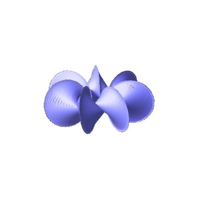
Figure 1. $a=2$ and $b=3$.

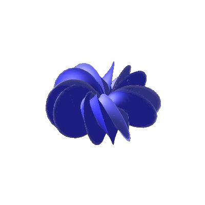
Figure 2. $a=\sqrt{2}$ and $b=3$.

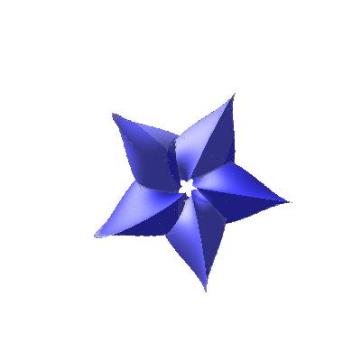
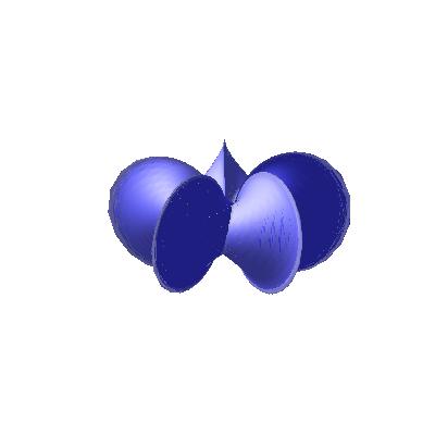
Figure 3. $a=\sqrt{3}$ and $b=\sqrt{2}$.

4. Constant angle surfaces

In this section we will complete our classification of helicoidal flat surfaces in $\mathbb{S}^{3}$, by establishing our second main theorem, that can be seen as a converse of Theorem 1. It is well known that the Hopf map $h:\mathbb{S}^{3}\to\mathbb{S}^{2}$ is a Riemannian submersion and the standard orthogonal basis of $\mathbb{S}^{3}$

$$E_{1}(z,w)=i(z,w),\ \ E_{2}(z,w)=i(-\overline{w},\overline{z}),\ \ E_{3}(z,w)=(-\overline{w},\overline{z})$$

has the property that $E_{1}$ is vertical and $E_{2}$, $E_{3}$ are horizontal. The vector field $E_{1}$, usually called the Hopf vector field, is an unit Killing vector field.

Constant angle surface in $\mathbb{S}^{3}$ are those surfaces whose its unit normal vector field makes a constant angle with the Hopf vector field $E_{1}$. The next result states that flatness of a helicoidal surface in $\mathbb{S}^{3}$ turns out to be equivalent to constant angle surface.

Proposition 3.

A helicoidal surface in $\mathbb{S}^{3}$, locally parametrized by (4) and with the profile curve $\gamma$ parametrized by (6), is a flat surface if and only if it is a constant angle surface.

Proof.

Let us consider the Hopf vector field

$$E_{1}(x_{1},x_{2},x_{3},x_{4})=(-x_{2},x_{1},-x_{4},x_{3}),$$

and let us denote by $\nu$ the angle between $E_{1}$ and the normal vector field $N$ along the surface given in (5). Along the parametrization (4), we can write the vector field $E_{1}$ as

$$E_{1}(X(t,s))=\phi_{\alpha,\beta}(t)(-x_{2},x_{1},0,x_{3}).$$

Then, since $\phi_{\alpha,\beta}(t)\in O(4)$, we have

$$\langle N,E_{1}\rangle(t,s)=\langle N,E_{1}\rangle(s)=(\beta-\alpha)\frac{x_{3}x_{3}^{\prime}}{\sqrt{\beta^{2}x_{3}^{2}+\alpha^{2}(x_{3}^{\prime})^{2}}}.$$

By considering the parametrization (6) for the profile curve $\gamma$, the angle $\nu=\nu(s)$ between $N$ and $E_{1}$ is given by

(19) $$\cos\nu(s)=(\beta-\alpha)\frac{\varphi^{\prime}\sin\varphi\cos\varphi}{\sqrt{\beta^{2}\sin^{2}\varphi+\alpha^{2}(\varphi^{\prime})^{2}\cos^{2}\varphi}}.$$

By taking the derivative in (19), we have

$$\frac{d}{ds}(\cos\nu(s))=\frac{(\beta-\alpha)\big{(}\beta^{2}\varphi^{\prime\prime}\sin^{3}\varphi\cos\varphi-\beta^{2}(\varphi^{\prime})^{2}\sin^{4}\varphi+\alpha^{2}(\varphi^{\prime})^{2}\cos^{4}\varphi\big{)}}{\big{(}\beta^{2}\sin^{2}\varphi+\alpha^{2}(\varphi^{\prime})^{2}\cos^{2}\varphi\big{)}^{\frac{3}{2}}},$$

and the conclusion follows from the Proposition 1. ∎

Given a number $\epsilon>0$, let us recall that the Berger sphere $\mathbb{S}^{3}_{\epsilon}$ is defined as the sphere $\mathbb{S}^{3}$ endowed with the metric

(20) $$\langle X,Y\rangle_{\epsilon}=\langle X,Y\rangle+(\epsilon^{2}-1)\langle X,E_{1}\rangle\langle Y,E_{1}\rangle,$$

where $\langle,\rangle$ denotes de canonical metric of $\mathbb{S}^{3}$. We define constant angle surface in $\mathbb{S}^{3}_{\epsilon}$ in the same way that in the case of $\mathbb{S}^{3}$. Constant angle surfaces in the Berger spheres were characterized by Montaldo and Onnis [17]. More precisely, if $M$ is a constant angle surface in the Berger sphere, with constant angle $\nu$, then there exists a local parametrization $F(u,v)$ given by

(21) $$F(u,v)=A(v)b(u),$$

where

(22) $$b(u)=\big{(}\sqrt{c_{1}}\cos(\alpha_{1}u),\sqrt{c_{1}}\sin(\alpha_{1}u),\sqrt{c_{2}}\cos(\alpha_{2}u),\sqrt{c_{2}}\sin(\alpha_{2}u)\big{)}$$

is a geodesic curve in the torus $\mathbb{S}^{1}(\sqrt{c_{1}})\times\mathbb{S}^{1}(\sqrt{c_{2}})$, with

$$c_{1,2}=\frac{1}{2}\mp\frac{\epsilon\cos\nu}{2\sqrt{B}},\ \alpha_{1}=\frac{2B}{\epsilon}c_{2},\ \alpha_{2}=\frac{2B}{\epsilon}c_{1},\ B=1+(\epsilon^{2}-1)\cos^{2}\nu,$$

and

(23) $$A(v)=A(\xi,\xi_{1},\xi_{2},\xi_{3})(v)$$

is a $1$-parameter family of $4\times 4$ orthogonal matrices given by

$$A(v)=A(\xi)\cdot\tilde{A}(v),$$

where

$$A(\xi)=\left(\begin{array}[]{cccc}1&0&0&0\\ 0&1&0&0\\ 0&0&\sin\xi&\cos\xi\\ 0&0&-\cos\xi&\sin\xi\end{array}\right)$$

and

$$\tilde{A}(v)=\left(\begin{array}[]{rrrr}\cos\xi_{1}\cos\xi_{2}&-\cos\xi_{1}\sin\xi_{2}&\sin\xi_{1}\cos\xi_{2}&-\sin\xi_{1}\sin\xi_{3}\\ \cos\xi_{1}\sin\xi_{2}&-\cos\xi_{1}\cos\xi_{2}&\sin\xi_{1}\sin\xi_{3}&\sin\xi_{1}\cos\xi_{3}\\ -\sin\xi_{1}\cos\xi_{3}&\sin\xi_{1}\sin\xi_{3}&\cos\xi_{1}\cos\xi_{2}&\cos\xi_{1}\sin\xi_{2}\\ \sin\xi_{1}\sin\xi_{3}&-\sin\xi_{1}\cos\xi_{3}&-\cos\xi_{1}\sin\xi_{2}&\cos\xi_{1}\cos\xi_{2}\end{array}\right),$$

$\xi$ is a constant and the functions $\xi_{i}(v)$, $1\leq i\leq 3$, satisfy

(24) $$\cos^{2}(\xi_{1}(v))\xi_{2}^{\prime}(v)-\sin^{2}(\xi_{1}(v))\xi_{3}^{\prime}(v)=0.$$

In the next result we obtain another relation between the function $\xi_{i}$, given in (23), and the angle function $\nu$.

Proposition 4.

The functions $\xi_{i}(v)$, given in (23), satisfy the following relation:

(25) $$(\xi_{1}^{\prime}(v))^{2}+(\xi_{2}^{\prime}(v))^{2}\cos^{2}(\xi_{1}(v))+(\xi_{3}^{\prime}(v))\sin^{2}(\xi_{1}(v))=\sin^{2}\nu,$$

where $\nu$ is the angle function of the surface $M$.

Proof.

With respect to the parametrization $F(u,v)$, given in (21), we have

$$F_{v}=A^{\prime}(v)\cdot b(u)=A(\xi)\cdot\tilde{A}^{\prime}(v)\cdot b(u).$$

We have $\langle F_{v},F_{v}\rangle=\sin^{2}\nu$ (cf. [17]). On the other hand, if we denote by $c_{1}$, $c_{2}$, $c_{3}$, $c_{4}$ the columns of $\tilde{A}$, we have

$$\langle F_{v},F_{v}\rangle|_{u=0}=g_{11}\langle c_{1}^{\prime},c_{1}^{\prime}\rangle+g_{33}\langle c_{3}^{\prime},c_{3}^{\prime}\rangle.$$

As $\langle c_{1}^{\prime},c_{1}^{\prime}\rangle=\langle c_{3}^{\prime},c_{3}^{\prime}\rangle$, $\langle c_{1}^{\prime},c_{3}^{\prime}\rangle=0$ and $g_{11}+g_{33}=1$, a straightforward computation gives

$$\sin^{2}\nu = \langle F_{v},F_{v}\rangle=(g_{11}+g_{33})\langle c_{1}^{\prime},c_{1}^{\prime}\rangle$$

$$= (\xi_{1}^{\prime}(v))^{2}+(\xi_{2}^{\prime}(v))^{2}\cos^{2}(\xi_{1}(v))+(\xi_{3}^{\prime}(v))\sin^{2}(\xi_{1}(v)),$$

and we conclude the proof. ∎

Theorem 2.

Let $M$ be a helicoidal flat surface in $\mathbb{S}^{3}$, locally parametrized by (4), and whose profile curve $\gamma$ is given by (6). Then $M$ admits a new local parametrization such that the fundamental forms are given as in (9) and $\omega$ is a linear function.

Proof.

Consider the unit normal vector field $N$ associated to the local parametrization $X$ of $M$ given in (4). From Proposition 3, the angle between $N$ and the Hopf vector field $E_{1}$ is constant. Hence, it follows from [17] (Theorem 3.1) that $M$ can be locally parametrized as in (21). By taking $\epsilon=1$ in (20), we can reparametrize the curve $b$ given in (22) in such a way that the new curve is a base curve $\gamma_{a}$. In fact, by taking $\epsilon=1$, we obtain $B=1$, and so $\alpha_{1}=2c_{2}$ and $\alpha_{2}=2c_{1}$. This implies that $\|b^{\prime}(u)\|=2\sqrt{c_{1}c_{2}}$, because $c_{1}+c_{2}=1$. Thus, by writing $s=2\sqrt{c_{1}c_{2}}$, the new parametrization of $b$ is given by

$$b(s)=\frac{1}{\sqrt{1+a^{2}}}\left(a\cos\frac{s}{a},a\sin\frac{s}{a},\cos(as),\sin(as)\right),$$

where $a=\sqrt{c_{1}/c_{2}}$. On the other hand, we have

$$A(v)\cdot b(s)=A(\xi)X(v,s),$$

where $X(v,s)$ can be written as

$$X(v,s)=\frac{1}{\sqrt{1+a^{2}}}(x_{1},x_{2},x_{3},x_{4}),$$

with

(30) $$\begin{array}[]{rcl}x_{1}&=&a\cos\xi_{1}\cos\left(\dfrac{s}{a}+\xi_{2}\right)+\sin\xi_{1}\cos(as+\xi_{3}),\\ x_{2}&=&a\cos\xi_{1}\sin\left(\dfrac{s}{a}+\xi_{2}\right)+\sin\xi_{1}\sin(as+\xi_{3}),\\ x_{3}&=&-a\sin\xi_{1}\cos\left(\dfrac{s}{a}-\xi_{3}\right)+\cos\xi_{1}\cos(as-\xi_{2}),\\ x_{4}&=&-a\sin\xi_{1}\sin\left(\dfrac{s}{a}-\xi_{3}\right)+\cos\xi_{1}\sin(as-\xi_{2}).\\ \end{array}$$

On the other hand, the product $\phi_{\alpha,\beta}(t)\cdot X(v,s)$ can be written as

$$\phi_{\alpha,\beta}(t)\cdot X(v,s)=\frac{1}{\sqrt{1+a^{2}}}(z_{1},z_{2},z_{3},z_{4}),$$

where

(35) $$\begin{array}[]{rcl}z_{1}&=&a\cos\xi_{1}\cos\left(\dfrac{s}{a}+\xi_{2}+\alpha t\right)+\sin\xi_{1}\cos\left(as+\xi_{3}+\alpha t\right),\\ z_{2}&=&a\cos\xi_{1}\sin\left(\dfrac{s}{a}+\xi_{2}+\alpha t\right)+\sin\xi_{1}\sin\left(as+\xi_{3}+\alpha t\right),\\ z_{3}&=&-a\sin\xi_{1}\cos\left(\dfrac{s}{a}-\xi_{3}+\beta t\right)+\cos\xi_{1}\cos\left(as-\xi_{2}+\beta t\right),\\ z_{4}&=&-a\sin\xi_{1}\sin\left(\dfrac{s}{a}-\xi_{3}+\beta t\right)+\cos\xi_{1}\sin\left(as-\xi_{2}+\beta t\right).\end{array}$$

As the surface is helicoidal, we have

$$\phi_{\alpha,\beta}(t)\cdot X(v,s)=X(v(t),s(t)),$$

for some smooth functions $v(t)$ and $s(t)$, which satisfy the following equations:

(36) $$\xi_{2}(v(t))+\dfrac{s(t)}{a}=\xi_{2}(v)+\dfrac{s}{a}+\alpha t,$$

(37) $$\xi_{3}(v(t))+as(t)=\xi_{3}(v)+as+\alpha t,$$

(38) $$\dfrac{s(t)}{a}-\xi_{3}(v(t))=\dfrac{s}{a}-\xi_{3}(v)+\beta t,$$

(39) $$as(t)-\xi_{2}(v(t))=as-\xi_{2}(v)+\beta t.$$

It follows directly from (36) and (39) that

(40) $$s(t)=s+\dfrac{a(\alpha+\beta)}{a^{2}+1}t.$$

Note that the same conclusion is obtained by using (37) and (38). By substituting the expression of $s(t)$ given in (40) on the equations (36) – (39), one has

(41) $$\xi_{2}(v(t))=\xi_{2}(v)+\left(\dfrac{a^{2}\alpha-\beta}{a^{2}+1}\right)t,$$

(42) $$\xi_{3}(v(t))=\xi_{3}(v)+\left(\dfrac{\alpha-a^{2}\beta}{a^{2}+1}\right)t.$$

From now on we assume that $v^{\prime}(t)\neq 0$ since, otherwise, we would have

$$\frac{s(t)}{a}=\frac{s}{a}+\alpha t=\frac{s}{a}+\beta t\quad\text{and}\quad as(t)=as+\alpha t=as+\beta t.$$

But the equalities above imply that $a^{2}=1$, which contradicts the definition of base curve in (11). Thus, it follows from (41) and (42) that

(43) $$\xi_{2}^{\prime}=\frac{a^{2}\alpha-\beta}{a^{2}+1}\cdot\frac{1}{v^{\prime}}\quad\text{and}\quad\xi_{3}^{\prime}=\frac{\alpha-a^{2}\beta}{a^{2}+1}\cdot\frac{1}{v^{\prime}}.$$

Therefore, from (24) and (43) we obtain

(44) $$\cos^{2}(\xi_{1}(v))(a^{2}\alpha-\beta)=\sin^{2}(\xi_{1}(v))(\alpha-a^{2}\beta).$$

As $a>1$, one has $a^{2}\alpha-\beta\neq 0$ or $\alpha-a^{2}\beta\neq 0$, and we conclude from (44) that $\xi_{1}(v)$ is constant. In this case, there is a constant $b>1$ such that $\cos^{2}\xi_{1}=\dfrac{b^{2}}{1+b^{2}}$ and $\sin^{2}\xi_{1}=\dfrac{1}{1+b^{2}}$. Therefore, it follows from (24) that

(45) $$\xi_{2}(v)=\dfrac{1}{b^{2}}\xi_{3}(v)+d,$$

for some constant $d$. On the other hand, if $\cos\xi_{1}\neq 0$, it follows from (24) that

(46) $$(\xi_{2}^{\prime}(v))^{2}=\tan^{4}\xi_{1}\cdot(\xi_{3}^{\prime}(v))^{2}.$$

By substituting (46) in (25) we obtain

$$\tan^{2}\xi_{1}\cdot(\xi_{3}^{\prime}(v))^{2}=\sin^{2}\nu,$$

ant this implies that we can choose $\xi_{3}(v)=bv$, and from (42) we obtain

(47) $$v(t)=v+\frac{\alpha-a^{2}\beta}{b(a^{2}+1)}t.$$

Moreover, from (45), the equation $\xi_{2}(v(t))=\dfrac{1}{b^{2}}\xi_{3}(v(t))+d$ implies that

(48) $$\dfrac{1}{b^{2}}=\dfrac{a^{2}\alpha-\beta}{\alpha-a^{2}\beta},$$

and from (48) we obtain the same relation (18) between $\alpha$ and $\beta$. This relation, when substituted in (40) and (47), gives

$$s(t)=s+\frac{a(b^{2}-1)}{a^{2}b^{2}-1}\beta t\quad\text{and}\quad v(t)=v+\frac{b(1-a^{2})}{a^{2}b^{2}-1}\beta t,$$

that coincide with the expressions in (17). Finally, from the relation (45) we obtain $\xi_{2}(v)=\frac{v}{b}-\frac{\pi}{2}$. By taking $\xi=\frac{\pi}{2}$ and $\xi_{1}(v)=\arcsin\left(\frac{1}{\sqrt{1+b^{2}}}\right)$, the new parametrization $F(u,v)$ thus obtained coincides with $Y(u,v)$ given in (16), up to isometries of $\mathbb{S}^{3}$ and linear reparametrization. The conclusion follows from Theorem 1. ∎

5. Conformally flat hypersurfaces

In this section, it will presented an application of the classification result for helicoidal flat surfaces in $\mathbb{S}^{3}$ in a geometric description for conformally flat hypersurfaces in four-dimensional space forms.

The problem of classifying conformally flat hypersurfaces in space forms has been investigated for a long time, with special attention on $4$-dimensional space forms. In fact, any surface in $\mathbb{R}^{3}$ is conformally flat, since it can be parametrized by isothermal coordinates. On the other hand, Cartan [4] gave a complete classification of conformally flat hypersurfaces into a $(n+1)$-dimensional space form, with $n+1\geq 5$. Such hypersurfaces are quasi-umbilic, i.e., one of the principal curvatures has multiplicity at least $n-1$. In the same paper, Cartan showed that the quasi-umbilic surfaces are conformally flat, but the converse does not hold. Since then, there has been an effort to obtain a classification of hypersurfaces with three distinct principal curvatures.

Lafontaine [14] considered hypersurfaces of type $M^{3}=M^{2}\times I\subset\mathbb{R}^{4}$ and obtained the following classes of conformally flat hypersurfaces: (a) $M^{3}$ is a cylinder over a surface, where $M^{2}\subset\mathbb{R}^{3}$ has constant curvature; (b) $M^{3}$ is a cone over a surface in the sphere, where $M^{2}\subset\mathbb{S}^{3}$ has with constant curvature; (c) $M^{3}$ is obtained by rotating a constant curvature surface of the hyperbolic space and $M^{2}\subset\mathbb{H}^{3}\subset\mathbb{R}^{4}$, where $\mathbb{H}^{3}$ is the half space model (see [22] for more details).

Hertrich-Jeromin [11] established a correspondence between conformally flat hypersufaces in space forms, with three distinct principal curvatures, and solutions $(l_{1},l_{2},l_{3}):U\subset\mathbb{R}^{3}\rightarrow\mathbb{R}$ for the Lamé’s system [15]

(49) $$\begin{array}[]{rcl}l_{i,x_{j}x_{k}}-\dfrac{l_{i,x_{j}}l_{j,x_{k}}}{l_{j}}-\dfrac{l_{i,x_{k}}l_{k,x_{j}}}{l_{k}}&=&0,\\ \left(\dfrac{l_{i,x_{j}}}{l_{j}}\right)_{,x_{j}}+\left(\dfrac{l_{j,x_{i}}}{l_{i}}\right)_{,x_{i}}+\dfrac{l_{i,x_{k}}l_{j,x_{k}}}{l_{k}^{2}}&=&0,\end{array}$$

where $i,j,k$ are distinct indices that satisfies the condition

(50) $$l_{1}^{2}-l_{2}^{2}+l_{3}^{2}=0$$

known as Guichard condition. In this case, the correspondent coformally flat hypersurface in $M^{4}_{K}$ is parametrized by curvature lines, with induced metric given by

$$g=e^{2u}\left\{l_{1}^{2}(dx_{1})^{2}+l_{1}^{2}(dx_{1})^{2}+l_{3}^{2}(dx_{3})^{2}\right\}.$$

In [6] the second author and Tenenblat obtained solutions of Lamé’s system (49) that are invariant under symmetry groups. Among the solutions, there are those that are invariant under the action of the 2-dimensional subgroup of translations and dilations and depends only on two variables:

1. $l_{1}=\lambda_{1},\;l_{2}=\lambda_{1}\cosh(b\xi+\xi_{0}),\;l_{3}=\lambda_{1}\sinh(b\xi+\xi_{0})$, where $\xi=\alpha_{2}x_{2}+\alpha_{3}x_{3}$, $\alpha_{2}^{2}+\alpha_{3}^{2}\neq 0$ and $b,\,\xi_{0}\in\mathbb{R}$ ;

2. $l_{2}=\lambda_{2},\;l_{1}=\lambda_{2}\cos\varphi(\xi),\;l_{3}=\lambda_{2}\sin\varphi(\xi)$, where $\xi=\alpha_{1}x_{1}+\alpha_{3}x_{3}$, $\alpha_{1}^{2}+\alpha_{3}^{2}\neq 0$ and $\varphi$ is one of the following functions:

   1. $\varphi(\xi)=b\xi+\xi_{0}$, if $\alpha_{1}^{2}\neq\alpha_{3}^{2}$, where $\xi_{0},\,b\in\mathbb{R}$;

   2. $\varphi$ is any function of $\xi$, if $\alpha_{1}^{2}=\alpha_{3}^{2}$;

3. $l_{3}=\lambda_{3},\;l_{2}=\lambda_{3}\cosh(b\xi+\xi_{0}),\;l_{1}=\lambda_{3}\sinh(b\xi+\xi_{0})$, where $\xi=\alpha_{1}x_{1}+\alpha_{2}x_{2}$, $\alpha_{1}^{2}+\alpha_{2}^{2}\neq 0$ and $b,\,\xi_{0}\in\mathbb{R}$.

It is known (see [22]) that the solutions that do not depend on one of the variables are associated to the products given by Lafontaine. For the solutions given in (b), further geometric solutions can be obtained with the classification result for helicoidal falt surfaces in $\mathbb{S}^{3}$. These solutions are associated to conformally flat hypersurfaces that are conformal to the products $M^{2}\times I\subset\mathbb{R}^{4}$ given by

$$M^{2}\times I=\left\{tp:0<t<\infty,p\in M^{2}\subset\mathbb{S}^{3}\right\},$$

where $M^{2}$ is a flat surface in $S^{3}$, parametrized by lines of curvature, whose first and second fundamental forms are given by

(51) $$\begin{array}[]{rcl}I&=&\sin^{2}(\xi+\xi_{0})dx_{1}^{2}+\cos^{2}(\xi+\xi_{0})dx_{3}^{2},\\ II&=&\sin(\xi+\xi_{0})\cos(\xi+\xi_{0})(dx_{1}^{2}-dx_{3}^{2}),\end{array}$$

which are, up to a linear change of variables, the fundamental forms that are considered in this paper. Therefore, as an application of the characterization of helicoidal flat surfaces in terms of first and second fundamental forms, one has the following theorem:

Theorem 3.

Let $l_{2}=\lambda_{2},\;l_{1}=\lambda_{2}\cos\xi+\xi_{0},\;l_{3}=\lambda_{2}\sin\xi+\xi_{0}$ be solutions of the Lamé’s sytem, where $\xi=\alpha_{1}x_{1}+\alpha_{3}x_{3}$ and $\alpha_{1},\,\alpha_{3},\,\lambda_{2},\,\xi_{0}$ are real constants with $\alpha_{1}\cdot\alpha_{3}\neq 0$. Then the associated conformally flat hypersurfaces are conformal to the product, $M^{2}\times I$, where $M^{2}\subset\mathbb{S}^{3}$ is locally congruent to helicoidal flat surface.

References

• [1] Aledo, J., Gálvez, J., and Mira, P. A d’alembert formula for flat surfaces in the 3-sphere. Journal of Geometric Analysis 19, 2 (2009), 211–232.
• [2] Baikoussis, C., and Koufogiorgos, T. Helicoidal surfaces with prescribed mean or Gaussian curvature. J. Geom. 63, 1-2 (1998), 25–29.
• [3] Bianchi, L. Sulle superficie a curvatura nulla in geometria ellittica. Ann. Mat. Pura Appl. 24 (1896), 93–129.
• [4] Cartan, E. La déformation des hypersurfaces dans l’éspace conforme réel à $n\geq 5$ dimensions. Bull. Soc. Math. France 45 (1917), 57–121. (Euvres Complètes Partie 3, Vol. 1, S. 221, Paris 1955).
• [5] do Carmo, M. P., and Dajczer, M. Helicoidal surfaces with constant mean curvature. Tôhoku Math. J. (2) 34, 3 (1982), 425–435.
• [6] dos Santos, J. P., and Tenenblat, K. The symmetry group of Lamé’s system and the associated Guichard nets for conformally flat hypersurfaces. SIGMA Symmetry Integrability Geom. Methods Appl. 9 (2013), Paper 033, 27.
• [7] Edelen, N. A conservation approach to helicoidal surfaces of constant mean curvature in $\mathbb{R}^{3}$, $\mathbb{S}^{3}$ and $\mathbb{H}^{3}$. arXiv:1110.1068.
• [8] Edelen, N., and Solomon, B. Constant mean curvature, flux conservation, and symmetry. Pacific J. Math. 274, 1 (2015), 53–72.
• [9] Gálvez, J. A. Isometric immersions of $\mathbb{R}^{2}$ into $\mathbb{R}^{4}$ and perturbation of hopf tori. Math. Z. 266, 1, 207–227.
• [10] Gálvez, J. A. Surfaces of constant curvature in 3-dimensional space forms. Mat. Contemp. 37 (2009), 1–42.
• [11] Hertrich-Jeromin, U. On conformally flat hypersurfaces and Guichard’s nets. Beirtrage zur Algebra und Geometrie 35, 2 (1994), 315–331.
• [12] Kitagawa, Y. Periodicity of the asymptotic curves on flat tori in $S^{3}$. J. Math. Soc. Japan 40, 3 (1988), 457–476.
• [13] Kokubu, M., Umehara, M., and Yamada, K. Flat fronts in hyperbolic 3-space. Pacific J. Math. 216, 2 (2004), 149–175.
• [14] Lafontaine, J. Conformal geometry from Riemannian viewpoint. In Conformal geometry, vol. E12 of Aspects of Math., (R.S. Kulkarni and U. Pinkall, eds. ), Max-Plank-Ins. fiir Math. Vieweg, Braunschweig, 1988, pp. 65–92.
• [15] Lamé, G. Leçons sur les coordonnés curvilignes et leurs diverses applications. Mallet-Bachelier, 1859. 73-78.
• [16] Martínez, A., dos Santos, J. P., and Tenenblat, K. Helicoidal flat surfaces in hyperbolic 3-space. Pacific J. Math. 264, 1 (2013), 195–211.
• [17] Montaldo, S., and Onnis, I. Helix surfaces in the Berger sphere. Israel J. Math. 201, 2 (2014), 949–966.
• [18] Palmer, B., and Perdomo, O. M. Rotating drops with helicoidal symmetry. Pacific J. Math. 273, 2 (2015), 413–441.
• [19] Perdomo, O. M. Helicoidal minimal surfaces in $\mathbb{R}^{3}$. Illinois J. Math. 57, 1 (2013), 87–104.
• [20] Ripoll, J. B. Uniqueness of minimal rotational surfaces in $S^{3}$. Amer. J. Math. 111, 4 (1989), 537–547.
• [21] Spivak, M. A comprehensive introduction to differential geometry. Vol. IV, second ed. Publish or Perish, Inc., Wilmington, Del., 1979.
• [22] Suyama, Y. Conformally flat hypersurfaces in Euclidean 4-space II. Osaka Math. J 42 (2005), 573–598.