Fusion of Array Operations at Runtime

Abstract

We address the problem of fusing array operations based on criteria such as shape compatibility, data reusability, and communication. We formulate the problem as a graph partition problem that is general enough to handle loop fusion, combinator fusion, and other types of subroutines.

I Introduction

Array operation fusion is a program transformation that combines, or fuses, multiple array operations into a kernel of operations. When it is applicable, the technique can drastically improve cache utilization through temporal data locality and enables other program transformations such as streaming and array contraction [5]. In scalar programming languages, such as C, array operation fusion typically corresponds to loop fusion where multiple computation loops are combined into a single loop. The effect is a reduction of array traversals (Fig. 1). Similarly, in functional programming languages it typically corresponds to fusing individual combinators. In array programming languages, such as HPF [11] and ZPL [2], fusing array operations are crucial, since a program written in these languages will consist almost exclusively of array operations. Lewis et al. demonstrates a execution time improvement of up to 400% when optimizing for array contraction at the array rather than the loop level [10].

However, not all fusions of operations are allowed. Consider the two loops in Fig. 1b; since the second loop traverses the result from the first loop in reverse, we must compute the complete result of the first loop before continuing to the second loop, preventing fusion. Clever analysis sometimes allows transforming the program into a form that is amenable to fusion, but such analysis is outside the scope of the present work. Throughout the remainder of this paper, we assume that any such optimizations have already been performed.

Deciding which operations to fuse together is the same as finding a partition of the set of operations in which the blocks obey the same execution dependency order as the individual operations, and in which no block contains two operations that may not be fused. Out of all such partitions, we want to find one that enables us to save the most computation or memory. It is not an easy problem, in part because fusibility is not transitive. That is, even when it is legal to fuse subroutines $x,y$ and $y,z$, it may be illegal for all three of $x,y,z$ to be executed together. Thus, one local decision can have global consequences on future possible partitions.

The problem can be stated in a quite general way: “Given a mixed graph, find a legal partition of vertices that cuts all non-directed edges and minimizes the cost of the partition.”. We call this problem the Weighted Subroutine Partition problem, abbreviated WSP.

⬇ #define N 1000 double A[N], B[N], T[N]; for(int i=0; i<N; ++i) T[i] = B[i] * A[i]; for(int i=0; i<N; ++i) A[i] += T[i];

(a)

⬇ #define N 1000 double A[N], B[N], T[N]; int j = N; for(int i=0; i<N; ++i) T[i] = B[i] * A[i]; for(int i=0; i<N; ++i) A[i] += T[–j];

(b)

⬇ for(int i=0; i<N; ++i){ T[i] = B[i] * A[i]; A[i] += T[i]; }

(c)

⬇ for(int i=0; i<N; ++i){ double t = B[i] * A[i]; A[i] += t; }

(d)

Figure 1: Loop fusion and array contraction in C.

The general formulation is applicable to a broad range of optimization objectives. The cost function can penalize any aspect of the partitions, e.g. data accesses, memory use, communication bandwidth, and/or communication latency. The only requirement to the cost function is monotonicity:

• Everything else equal, it must be cost neutral or a cost advantage to place two subroutines within the same partition block.

Similarly, the definition of partition legality is flexible.

• Any aspect of a pair of subroutines can make them illegal to have in the same partition block, such as preventing mixing of sequential and parallel loops, different array shapes, or access patterns.

• Subroutines may have dependencies that impose a partial order. Then a legal partition must observe this order, i.e. must not introduce cycles.

The remainder of the paper is structured as follows: In Section 3, we formally define the Weighted Subroutine Partition problem, which unifies array operation-, loop-, and combinator fusion, and prove that it is NP-hard. Section 4 shows how WSP is used to solve array operation fusion for the Bohrium automatic parallelization framework, and gives a correctness proof. In Section 5, we describe a branch-and-bound algorithm that computes an optimal solution, as well as two approximation algorithms that compute good results rapidly enough to use in JIT-compilation. All the algorithms are implemented in Bohrium, and work for any choice of monotonic cost function, which allows us to compare directly with other fusion schemes from the literature. Section 6 shows measurements performed on 15 benchmark programs, comparing both the optimal to the approximation schemes, and to three other fusion schemes.

II Related Work

The WSP problem presented in this paper generalizes the Weighted Loop Fusion (WLF) problem first described by Kennedy in [6] (by the name Fusion for Reuse). The method aims to maximize data locality through loop fusion (corresponding to the Max Locality cost model in Section VI-A). The WLF problem is described as a graph problem where vertices represent computation loops, directed edges represent data dependencies between loops, and undirected edges represent data sharing between loops. Edges that connect fusible loops have a non-negative weight that represents the cost saving associated with fusion of the two loops. Edges that connect non-fusible loops are marked as fuse-preventing. Now, the objective is to find a partition of the vertices into blocks such that no block has vertices connected with fuse-preventing edges and that minimize the weight sum of edges that connects vertices in different blocks.

Megiddo et al. have shown that it is possible to formulate the WLF problem as integer linear programming (ILP) [13]. Based on the WLF graph, the idea is to transform the edges into linear constraints that implement the dependency and fusibility between the vertices and transform weights into ILP objective variables. The values of the objective variables are either the values of the weights when the associated vertices are in different partitions or zero when in the same partition. The objective of the ILP is then to minimize the value of the objective variables . The problem is NP-hard, but the hope is that with an efficient ILP solver, such as lp-solve [1], and a modest problem size it might be practical as a compile time optimization. Darte et al. [4] proved that the WLF problem is NP-hard through a reduction from multiway cut [3]. Furthermore, since maximizing data locality may not maximize the number of array contractions(Fig. 21), they introduce an ILP formulation with the sole objective of maximizing the number of array contractions (the Max Contract cost model in Section VI-A).

Robinson et al. [14] describe an ILP scheme that combines the objectives of Megiddo and Darte: both maximizing data locality and array contractions while giving priority to data locality (corresponds to our Robinson cost model).

However, optimization using WLF has a significant limitation: it only allows static edge weights. That is, when building the WLF graph the values of edge weights are assigned once and for all. This limitation is the main reason that we needed to develop the Weighted Subroutine Partition formalism, because static edge weights are in fact inappropriate for accurate measurement of data locality.

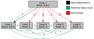
(a)

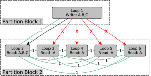
(b)

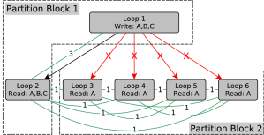
(c)

Figure 2: A WLF example where the objective is to maximize data locality. (a) shows the initial graph. (b) shows a partition where loop 1 is in one block and loops 2-6 are in another block. (c) shows a partition where loops 1-2 are in one block and loops 3-6 are in another block.

Consider the WLF example in Fig. 2, which consist of six loops and three arrays $A,B,C$ of size $1$. The objective is to maximize data locality, represented by weight edges connecting the loops that access the same arrays. Fig. 2b shows the optimal WLF solution to the example, which reduces the total weight from 13 to 3. However, the actual number of array accesses is only reduced from 10 to 7. A better strategy is to fuse loop 1-2 (Fig. 2c), which will reduce the actual number of array accesses from 10 to 4.

The problem with the WLF formulation here is that all the loops that read the same data must be pair-wise connected with a weight, leading to over-estimating potential data reuse. In the Weighted Subroutine Partition formulation, we work with partitions instead of individual merges, and assign a cost to a partition as a whole. The cost-savings of a merge is then the difference in cost between the partitions before and after merging, allowing accurate descriptions of data-reuse through the costs function.

III The Weighted Subroutine Partition Problem

The Weighted Subroutine Partition (WSP) problem is an extension of the The Weighted Loop Fusion Problem [6] where we include the weight function in the problem formulation. In this section, we will formally define the WSP problem and show that it is NP-hard.

Definition 1 (WSP graph).

A WSP graph is a triplet $G=(V,E_{d},E_{f})$ such that $(V,E_{d})$ is a directed acyclic graph describing dependency order, and $(V,E_{f})$ is an undirected graph of forbidden edges.

Definition 2 (WSP order).

A WSP graph, $G=(V,E_{d},E_{f})$, induces a partial order $\mathrel{\vbox{\offinterlineskip\halign{\hfil#\hfil\cr$\scriptscriptstyle d$\cr\kern 0.0pt\cr$<$\cr}}}$ on $V$ as follows: $v\mathrel{\vbox{\offinterlineskip\halign{\hfil#\hfil\cr$\scriptscriptstyle d$\cr\kern 0.0pt\cr$<$\cr}}}v^{\prime}$ iff there exists a path from $v$ to $v^{\prime}$ in $(V,E_{d})$. Since $(V,E_{d})$ is acyclic, this partial order is strict.

Definition 3 (Partitions).

A partition of a set $V$ is a set $P=\{B_{1},B_{2},\ldots,B_{k}\}$ such that $V$ is the disjoint union of the blocks $B_{1},\ldots,B_{k}$. The set $\Pi_{V}$ of all partitions of $V$ is partially ordered as $P\leq P^{\prime}$ iff $\forall B\in P\exists B^{\prime}\in P^{\prime}\colon B\subseteq B^{\prime}$, i.e. if each block in $P$ is a subset of a block in $P^{\prime}$.

The set of partitions $\Pi_{V}$ is a lattice with bottom and top elements $\bot=\{V\}$ and $\top=\{\{V\}\}$. The successors to a partition $P$ in the partition order are those partitions that are identical to $P$ except for merging two of the blocks. Conversely, splitting a block results in a predecessor. We write $P\prec P^{\prime}$ if $P^{\prime}$ is a successor to $P$. This defines a binary merge operator:

Definition 4 (Block merge operator).

Given a partition $P=\{B_{1},B_{2},\ldots\}$, define $P/(B_{1},B_{2})=\{B_{1}\cup B_{2},\ldots\}$ to be the successor to $P$ in which $B_{1}$ and $B_{2}$ are merged and all other blocks are left the same.

Definition 5 (Legal partition).

Given a WSP graph, $G=(V,E_{d},E_{f})$, we say that the partition $P\in\Pi_{V}$ is legal when the following holds for every block $B\in P$:

1. $\nexists v_{1},v_{2}\in B:(v_{1},v_{2})\in E_{f}$, i.e.  no block contains both endpoints of a forbidden edge.

2. If $v_{1}\mathrel{\vbox{\offinterlineskip\halign{\hfil#\hfil\cr$\scriptscriptstyle d$\cr\kern 0.0pt\cr$<$\cr}}}v_{2}\mathrel{\vbox{\offinterlineskip\halign{\hfil#\hfil\cr$\scriptscriptstyle d$\cr\kern 0.0pt\cr$<$\cr}}}v_{3}$ and $v_{1},v_{3}\in B$ then $v_{2}\in B$, i.e.  the directed edges between blocks must not form cycles.

Definition 6 (WSP cost).

Given a partition, $P$, of vertices in a WSP graph, a cost function $\mathsf{cost}(P)$ returns the cost of the partition and respects the following conditions:

1. $\mathsf{cost}(P)\geq 0$

2. $P\leq P^{\prime}\implies\mathsf{cost}(P)\geq\mathsf{cost}(P^{\prime})$

Definition 7 (WSP problem).

Given a WSP graph, $G=(V,E_{d},E_{f})$, and a cost function, $\mathsf{cost}(P)$, the WSP problem is the problem of finding a legal partition, $P^{*}$, of $V$ with minimal cost:

$$P^{*}\in\operatornamewithlimits{argmin}_{P\in\hat{\Pi}_{V}}\mathsf{cost}(P)$$ (1)

where $\hat{\Pi}_{V}$ denotes the set of legal partitions of $V$.

III-A Complexity

In order to prove that the WSP problem is NP-hard, we perform a reduction from the Multiway Cut Problem [3], which Dahlhaus et al. has shown is NP-hard for fixed $k\geq 3$.

Definition 8 (Multiway Cut).

Given a tuple $(V,E,S,w)$ consisting of a graph $(V,E)$, a terminal set $S=\{s_{1},\ldots,s_{k}\}$ of vertices, and a non-negative weight $w(u,v)$ for each edge $(u,v)\in E$, a multiway cut is an edge set $E^{\prime}$ the removal of which leaves each terminal in separate components. The solutions to the MWC problem are the multiway cuts of minimal total weight.

Theorem 1.

The WSP problem is NP-hard for graphs $G=(V,E_{d},E_{f})$ that have a chain of three or more edges in $E_{f}$.

Proof.

We prove NP-hardness through a reduction from multiway cut. Given an MWC-instance, $(V,E,S,w)$, we build a WSP-instance as follows. Let $G=(V,E_{d},E_{f})$, $E_{f}=\{(s_{i},s_{j}):1\leq i<j\leq k\}$, and $E_{d}=\emptyset$. Define the cut of a partition as the set of edges that connect the blocks:

$$\mathsf{cut}(P)=\left\{(u,v)\in E_{f}\middle|\nexists B\in P:(u,v)\in B\right\}$$

The cuts of the legal WSP partitions $\hat{\Pi}_{V}$ are exactly the set of multiway cuts:

• The set of directed edges in $E_{d}$ is empty, which makes Def. 2 and Def. 5(2) trivially satisfied.

• The fuse-preventing edges $E_{f}$ connect each terminal in $S$ and no other vertices. Hence, by Def. 5(1), $\hat{\Pi_{V}}$ are exactly those partitions for which no block contains two terminals.

Let now the cost function be the total weight of the cut:

$$\mathsf{cost}(P)=\sum_{(u,v)\in\mathsf{cut}(P)}w(u,v)$$

This is a valid WSP cost function (by Def. 6): it is non-negative, and if $P\leq P^{\prime}$ in the partition order, then $\mathsf{cut}(P)\supseteq\mathsf{cut}(P^{\prime})$, whereby $\mathsf{cost}(P)\geq\mathsf{cost}(P^{\prime})$. Since $\mathsf{cost}(P)$ is the MWC total weight, Eq. (1) gives the multiway cuts of minimal total weight, concluding the proof. ∎

IV WSP used to optimize array operation fusion in Bohrium

Stating the WSP problem formulation in a general way allows a great deal of flexibility, as long as the cost function is monotonic. In this section, we use WSP to solve a concrete optimization problem, demonstrating its real world use. The concrete problem is an optimization phase within the Bohrium runtime system [9] in which a set of array operations are partitioned into computation kernels – the Fusion of Array Operations (FAO) problem:

Definition 9.

Given a set of array operations, $A$, equipped with a strict partial order imposed by the data dependencies between them, $(A,\mathrel{\vbox{\offinterlineskip\halign{\hfil#\hfil\cr$\scriptscriptstyle d$\cr\kern 0.0pt\cr$<$\cr}}})$, find a partition, $P$, of $A$ for which:

1. All operations within a block in $P$ are fusible (Def. 11)

2. For all blocks, $B\in P$, if $a_{1}\mathrel{\vbox{\offinterlineskip\halign{\hfil#\hfil\cr$\scriptscriptstyle d$\cr\kern 0.0pt\cr$<$\cr}}}a_{2}\mathrel{\vbox{\offinterlineskip\halign{\hfil#\hfil\cr$\scriptscriptstyle d$\cr\kern 0.0pt\cr$<$\cr}}}a_{3}$ and $a_{1},a_{3}\in B$ then $a_{2}\in B$. (I.e. the partition obeys dependency order).

3. The cost of the partition (Def. 13) is minimal.

In the following, we will provide a brief description of Bohrium and show that the WSP problem solves the FAO problem (Theorem 2).

IV-A Fusion of Array Operations in Bohrium

⬇ 1import bohrium as bh 2 3def synthetic(): 4 A = bh.zeros(4) 5 B = bh.zeros(4) 6 D = bh.zeros(5) 7 E = bh.zeros(5) 8 A += D[:-1] 9 A[:] = D[:-1] 10 B += E[:-1] 11 B[:] = E[:-1] 12 T = A * B 13 bh.maximum(T, E[1:], out=D[1:]) 14 bh.minimum(T, D[1:], out=E[1:]) 15 return D 16print synthetic()

(a)

⬇ 1COPY A, 0 2COPY B, 0 3COPY D, 0 4COPY E, 0 5ADD A, A, D[:-1] 6COPY A, D[:-1] 7ADD B, B, E[:-1] 8COPY B, E[:-1] 9MUL T, A, B 10MAX D[1:], T, E[1:] 11MIN E[1:], T, D[1:] 12DEL A 13DEL B 14DEL E 15DEL T 16SYNC D 17DEL D

(b)

Figure 3: A Python application that utilizes the Bohrium runtime system. In order to demonstrate various challenges and trade-offs, the application is synthetic. (a) shows the Python code and (b) shows the corresponding Bohrium array bytecode.

Bohrium is a computation backend for array programming languages and libraries that supports a range of languages, such as Python, C++, and .NET, and a range of computer architectures, such as CPU, GPU, and clusters of these. The idea is to decouple the domain specific frontend implementation from the hardware specific backend implementation in order to provide a high-productivity and high-performance framework.

Similar to NumPy [15], a Bohrium array operation operates on a set of inputs and produces a set of outputs [9]. Both input and output operands are views of arrays. An array view is a structured way to observe the whole or parts of an underlying base array. A base array is always a contiguous one-dimensional array whereas views can have any shape, stride, and dimensionality [9]. In the following, when we refer to an array, we mean an array view; when we refer to identical arrays, we mean identical array views that points to the same base array; and when we refer to overlapping arrays, we mean array views that points to some of the same elements in a common base array.

Fig. 3a shows a Python application that uses Bohrium as a drop-in replacement for NumPy. The application allocates and initiates four arrays (line 4-7), manipulates those arrays through array operations (line 8-14), and prints the content of one of the arrays (line 16).

As Bohrium is language agnostic, it translates the Python array operations into bytecode (Fig. 3b) that the Bohrium backend can execute. In the case of Python, the Python array operations and the Bohrium array bytecode is almost in one-to-one mapping. The first bytecode operand is the output array and the remaining operands are either input arrays or input literals. Since there is no scope in the bytecode, Bohrium uses DEL to destroy arrays and SYNC to move array data into the address space of the frontend language – in this case triggered by the Python print statement (Fig. 3a, line 16). There is no explicit bytecode for constructing arrays; on first encounter, Bohrium constructs them implicitly.

In the next phase, Bohrium partitions the list of array operations into blocks that consists of fusible array operations – the FAO problem. As long as the preceding constraints between the array operations are preserved, Bohrium is free to reorder them as it sees fit, making code optimizations based on data locality, array contraction, and streaming possible.

In the final phase, the hardware specific backend implementation JIT-compiles each block of array operations and executes them.

IV-A1 Fusibility

In order to utilize data-parallelism, Bohrium and most other array programming languages and libraries require data-parallelism of array operations that are to be executed together. The property ensures that the runtime system can calculate each output element independently without any communication between threads or processors. In Bohrium, all array operation must have this property.

We first introduce some operations that keep track of memory allocation, deallocation, reads, and writes:

Definition 10.

Given an array operation $f$, the notation $\mathsf{in}[f]$ denotes the set of arrays that $f$ reads; $\mathsf{out}[f]$ denotes the set of arrays that $f$ writes; $\mathsf{new}[f]$ denotes the set of new arrays that $f$ allocates; and $\mathsf{del}[f]$ denotes the set of arrays that $f$ deletes (or de-allocates).

Furthermore, given a set of array operations, $B$, we define the following:

$$\mathsf{out}[B] \equiv\operatornamewithlimits{\mathbin{\scalebox{1.6}{$\cup$}}}_{f\in B}\mathsf{out}[f]$$

$$\mathsf{in}[B] \equiv\operatornamewithlimits{\mathbin{\scalebox{1.6}{$\cup$}}}_{f\in B}\mathsf{in}[f]$$

$$\mathsf{new}[B] \equiv\operatornamewithlimits{\mathbin{\scalebox{1.6}{$\cup$}}}_{f\in B}\mathsf{new}[f]$$

$$\mathsf{del}[B] \equiv\operatornamewithlimits{\mathbin{\scalebox{1.6}{$\cup$}}}_{f\in B}\mathsf{del}[f]$$

$$\mathsf{ext}[B] \equiv(\mathsf{in}[B]\setminus\mathsf{new}[B])\sqcup(\mathsf{out}[B]\setminus\mathsf{del}[B])$$

Here, $\mathsf{ext}[B]$ gives the set of external data accesses. “$\sqcup$” is disjoint union: arrays that are both read and written are counted twice. DEL and SYNC are counted as having no input or output.

This allows us to formulate the data-parallelism property that determines when array operation fusion is allowed:

Definition 11.

A Bohrium array operation, $f$, is data parallel, i.e., each output element can be calculated independently, when the following holds:

$$\forall{i\in\mathsf{in}[f]},\forall{o,o^{\prime}\in\mathsf{out}[f]}:\\ (i\cap o=\emptyset\lor i=o)\land(o\cap o^{\prime}=\emptyset\lor o=o^{\prime})$$ (2)

In other words, if an input and an output or two output arrays overlaps, they must be identical.

Fusing array operation must preserve data-parallelism:

Definition 12.

In Bohrium, two array operations, $f$ and $f^{\prime}$, are said to be fusible when the following holds:

$$\forall i^{\prime}\in\mathsf{in}[f^{\prime}],\ \ \forall o\in\mathsf{out}[f]\colon i^{\prime}\cap o=\emptyset\lor i^{\prime}=o$$ (1)

$$\forall o^{\prime}\in\mathsf{out}[f^{\prime}],\forall o\in\mathsf{out}[f]\colon o^{\prime}\cap o=\emptyset\lor o^{\prime}=o$$ (2)

$$\forall o^{\prime}\in\mathsf{out}[f^{\prime}],\forall i\in\mathsf{in}[f]\colon o^{\prime}\cap i=\emptyset\lor o^{\prime}=i$$ (3)

It follows from Definition 11 that fusible operations are those that can be executed together without losing independent data-parallelism.

In addition to the data-parallelism property, the current implementation of Bohrium also requires that the length and dimensionality of the fusible array operations are the same.

IV-A2 Cost Model

The motivation of fusing array operations is to reduce the overall execution time. To accomplish this, Bohrium implements two techniques:

Data Locality

When a kernel accesses an array multiple times, Bohrium will only read and/or write to that array once, avoiding access to main memory. Consider the two for-loops in Fig. 1a that each traverse A and T. Fusing the loops avoids one traversal of A and one traversal of T (Fig. 1c). Furthermore, the compiler can reduce the access to the main memory by $2N$ elements since it can keep the last read element of A and T in register.

Array Contraction

When an array is created and destroyed within a single partition block, Bohrium will not allocate the array memory, but calculate the result in-place in one single temporary register variable per parallel computing thread. Consider the program transformation from Fig. 1a to 1d, in which, beside loop fusion, the temporary array $T$ is replaced by the scalar variable $t$. In this case, the transformation reduces the accessed elements with $3N$ and memory requirement by $N$ elements.

In order to utilize these optimization techniques, we introduce a WSP cost function that penalizes memory accesses from different partition blocks. For simplicity, we will not differentiate between reads and writes, and we will not count access to literals or register variables.

Definition 13.

In bohrium, the cost of a partition, $P=\{B_{1},B_{2},...,B_{k}\}$, of array operations is given by:

$$\mathsf{cost}(P)=\sum_{B\in P}\left\|\mathsf{ext}[B]\right\|$$ (3)

where the length $\left\|x\right\|$ is the total number of bytes accessed by the set of arrays in $x$.

The Bohrium cost-savings when merging two partition blocks depends only on the blocks:

Proposition 1 (Merge-savings).

Let $P$ be a partition and $P^{\prime}=P/(B_{1},B_{2})$ be its successor derived by merging $B_{1}$ and $B_{2}$. Using the cost function of Def. 13, the difference in cost between the two partitions is:

$$\mathsf{cost}(P)-\mathsf{cost}(P^{\prime})= \phantom{+}\,\,\left\|\mathsf{ext}[B_{1}]\cap\mathsf{ext}[B_{2}]\right\|$$

$$+\left\|\mathsf{new}[B_{1}]\cap\mathsf{in}[B_{2}]\right\|$$

$$+\left\|\mathsf{out}[B_{1}]\cap\mathsf{del}[B_{2}]\right\|$$ (4)

Since this cost reduction depends only on $B_{1}$ and $B_{2}$, we define a function, $\mathsf{saving}(B_{1},B_{2})$, that counts the savings from merging $B_{1}$ and $B_{2}$, which is independent of the rest of the partitions.

Proof.

If $P=\{B_{1},B_{2},\ldots,\}$ and $P^{\prime}=\{B_{1}\cup B_{2},\ldots\}$, then the reduction in cost is

$$\mathsf{cost}(P)-\mathsf{cost}(P^{\prime})=\left\|\mathsf{ext}(B_{1})\right\|+\left\|\mathsf{ext}(B_{2})\right\|-\left\|\mathsf{ext}(B_{1}\cup B_{2})\right\|$$

since all other blocks are the same. By using the fact that $B_{1}$ must be executed before $B_{2}$, whereby $\mathsf{in}[B_{1}]\cap\mathsf{new}[B_{2}]=\emptyset$ and $\mathsf{del}[B_{1}]\cap\mathsf{out}[B_{2}]=\emptyset$, as well as the $\mathsf{new}$’s and $\mathsf{del}$’s being disjoint, direct calculation yields Eq. 1. ∎

Note that Prop. 1 directly implies that the cost function of Def. 13 is positive and monotonically decreasing, as required by Def. 6. We next show how the problem can be formulated as a WSP instance.

IV-A3 Constructing a WSP-problem from Bohrium bytecode

Given a list $A$ of Bohrium array operations, a WSP problem $G=(V,E_{d},E_{f})$ is constructed as follows.

1. The data dependencies between array operations define a partial order: $a\mathrel{\vbox{\offinterlineskip\halign{\hfil#\hfil\cr$\scriptscriptstyle d$\cr\kern 0.0pt\cr$<$\cr}}}a^{\prime}$ iff $a^{\prime}$ must be executed before $a$.

2. Each array operation $a\in A$ defines a vertex $v(a)\in V$.

3. The dependency graph $E_{d}$ has an edge $(v(a),v(a^{\prime}))$ for each pair $a,a^{\prime}\in A$ with $a\mathrel{\vbox{\offinterlineskip\halign{\hfil#\hfil\cr$\scriptscriptstyle d$\cr\kern 0.0pt\cr$<$\cr}}}a^{\prime}$.

4. The fuse-prevention graph $E_{f}$ has an edge $(v(a),v(a^{\prime}))$ for each non-fusible pair $a,a^{\prime}\in A$.

The cost function is as in Def. 13, but note that it can be calculated incrementally using Prop. 1.

The complexity of this transformation is $O(V^{2})$ since we may have to check all pairs of array operations for dependecies, fusibility, and cost-saving, all of which is $O(1)$. Fig. 4 shows the trivial partition, $\bot$, of the Python example, where every array operation has its own block. The cost is 94.

IV-A4 WSP solves Fusion of Array Operations

Finally, we can show that a solution to the WSP problem also is a solution to the FAO problem.

Theorem 2.

WSP solves Fusion of Array Operations.

Proof.

It is clear from Def. 5 and the construction above that the legal partitions $\hat{\Pi}_{V}$ are exactly all those that fulfill Properties (1) and (2) of Def. 9. Thus, Def. 7 yields a global minimum for all such partitions, fulfilling also Def. 9(3). ∎

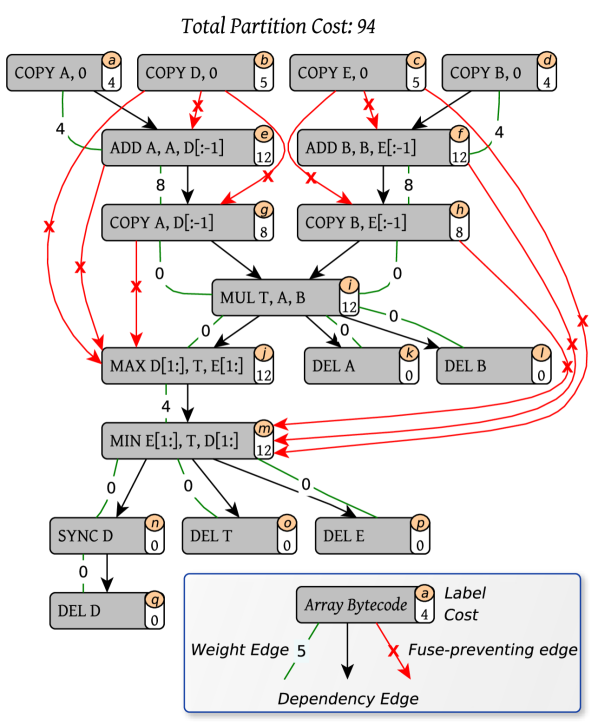
Figure 4: A partition graph of the Python application in Fig. 3. For illustrative proposes, the graph does not include ignored weight edges (cf. Fig. 5).

V Algorithms

In this section, we present an exact algorithm for finding an optimal solution to WSP (with exponential worst-case execution time), and two fast algorithms that find approximate solutions. We use the Python application shown in Fig. 3 to demonstrate the results of each partition algorithm.

V-A Partition graphs and chains of block merges

All three algorithms work on data structures called partition graphs, defined as follows:

Definition 14 (Partition graph).

Given a graph $G=(V,E)$ and a partition $P$ of $V$, the corresponding partition graph is the graph $\hat{G}(P)=(P,\hat{E}(P))$ that has an edge $(B,B^{\prime})$ if there is an edge $(u,v)\in E$ with $u\in B$ and $v\in B^{\prime}$. That is, the vertices are the blocks, connected by the edges that cross block boundaries.

From this we build the state needed in WSP computations:

Definition 15 (WSP state).

Given a WSP-instance $G=(V,E_{d},E_{f},\mathsf{cost})$ and a partition $P$, the WSP state is the partition graph $\hat{G}(P)=(P,\hat{E_{d}}(P),\hat{E_{f}}(P))$ together with a complete weighted graph $\hat{E_{w}}(P)$ with weights $w(B_{1},B_{2})=\mathsf{cost}(P)-\mathsf{cost}(P/(B_{1},B_{2}))$.

Notice that $w(B_{1},B_{2})=\mathsf{saving}(B_{1},B_{2})$ for the Bohrium cost function, as shown in Prop. 1, and does not require a full cost calculation.

Definition 16 (Merge operator on partition graphs).

We extend the merge operator of Def. 4 to partition graphs as $\hat{G}(P)/(B_{1},B_{2})=\hat{G}(P/(B_{1},B_{2}))$. This acts exactly as a vertex contraction on the partition graph.

The merge operator is commutative in the sense that the order in a sequence of successive vertex contractions doesn’t affect the result [16]. An auxiliary function, Merge, is used in each algorithm to update the state.

Definition 17.

Let $S=(\hat{G},\hat{E}_{w})$ be a WSP state. We define

$$\textsc{Merge}((S,u,v))=(\hat{G}/(u,v),\hat{E_{w}}^{\prime})$$

where $\hat{E_{w}}^{\prime}$ is the updated weight graph on the edges incident to the new vertex $z=u\cup v$.

The complexity of Merge is dominated by the weight update, which requires a $\mathsf{saving}{}$ computations per edge incident to the merged vertex, and is bounded by $\mathcal{O}\left(V^{2}\right)$. We next need a local condition for when a merge is allowed:

Lemma 1 (Legal merge).

Let $P_{1,2}=P/(B_{1},B_{2})$ be the successor to a legal partition $P\in\hat{\Pi}_{V}$, derived by merging blocks $B_{1}$ and $B_{2}$. Then $P_{1,2}\in\hat{\Pi}_{V}$ if and only if

1. $(B_{1},B_{2})\notin\hat{E_{f}}(P)$, and

2. there is no path of length $\geq 2$ from $B_{1}$ to $B_{2}$ in the partition graph $\hat{E_{d}}(P)$.

Proof.

Recall that $\hat{\Pi}_{V}$ is the subset of partitions in $\Pi_{V}$ that satisfy Def. 5. Because $P$ is legal, no block contains an edge in $E_{f}$. Hence $P_{1,2}$ obeys Def. 5(1) if and only if no two vertices $u\in B_{1}$ and $v\in B_{2}$ are connected in $E_{f}$, or equivalently, $(B_{1},B_{2})\notin\hat{E_{f}}(P)$.

Similarly, by assumption, there are no cycles in $\hat{E_{d}}(P)$. Thus, $P_{1,2}$ violates Def. 5(2) if and only if $\hat{E_{d}}(P)$ contains a path $B_{1}\to B^{\prime}\to\cdots\to B_{2}$, forming the cycle $B_{1,2}\to B^{\prime}\to\cdots\to B_{1,2}$ in $\hat{E_{d}}(P_{1,2})$ (where $B_{1,2}=B_{1}\cup B_{2}$). ∎

Proposition 2 (Reachability through legal merges).

Given two legal partitions $P<P^{\prime}$, there exists a successor chain $P\prec P_{1}\prec P_{2}\prec\cdots\prec P^{\prime}$ entirely contained in $\hat{\Pi}_{V}$, i.e. corresponding only to legal block merges.

Proof.

A successor chain $P\prec P_{1}\prec\cdots\prec P_{n-1}\prec P^{\prime}$ always exists in the total set of partitions $\Pi_{V}$, and all such chains are of the same length $n$. Any such chain contains no partition that violates Def. 5(1): each step is a merge, so once a fuse-preventing edge is placed inside a block, it would be included also in a block from $P^{\prime}$. Hence we only need to worry about Def. 5(2).

We now show by induction that a successor chain consisting of only legal partitions exists. First, if $P\prec P^{\prime}$, it is trivially so. Assume now that the statement is true for all $n\leq N$, and consider $P<P^{\prime}$ of distance $N+1$.

Pick any successor chain from $P$ to $P^{\prime}$. If any step violates Def. 5(2), then let $P_{i+1}=P_{i}/(B_{1},B_{2})$ be the first partition in the chain that does so. Then there is a path $B_{1}\to B\to\cdots\to B_{2}$ in the transitive reduction of $\hat{E_{d}}(P_{i})$. Because $P^{\prime}$ satisfies Def. 5(2), $B_{1}\cup B\cup B_{2}$ is contained in a block from $P^{\prime}$, whereby $P_{i+1}^{\prime}\equiv P_{i}/(B_{1},B)<P^{\prime}$. This merge introduces no cycles, because the path is in the transitive reduction. Now let $P_{i+1}^{\prime}\prec P_{i+2}^{\prime}\prec\cdots\prec P^{\prime}$ be a legal successor chain of length $N-i$, known to exist by hypothesis. Then $P\prec P_{1}\prec\cdots\prec P_{i}\prec P_{i+1}^{\prime}\prec\cdots\prec P^{\prime}$ is a length-$N+1$ successor chain consisting of only legal partitions, concluding the proof by induction. ∎

In particular, the optimal solutions can be reached in this way from the bottom partition $\bot=\{\{v_{1}\},\{v_{2}\},\ldots,\{v_{n}\}\}$, which we will use in the design of the algorithms.

Figure 5: A help function thet determines whether the weight edge, $e\in E_{w}[G]$

V-B Unintrusive Partition Algorithm

In order to reduce the size of the partition graph to be analyzed, we apply an unintrusive strategy where we merge vertices that are guaranteed to be part of an optimal solution. Consider the two vertices, $a,e$, in Fig. 4. The only beneficial merge possibility $a$ has is with $e$, so if $a$ is merged in the optimal solution, it is with $e$. Now, since fusing $a,e$ will not impose any restriction to future possible vertex merges in the graph, the two vertices are said to be unintrusively fusible. We formalize this property using the non-fusible sets:

Definition 18 ($\theta$, non-fusible set).

The non-fusible set, $\theta[b]$ for a block $b$ is the set of blocks connected with $b$ in $\hat{E_{d}}$ through a path containing a non-fusible edge.

Theorem 3.

Given a partition graph $\hat{G}$, let $z=u\cup v$ be the merged vertex in $\hat{G}/(u,v)$. The vertices $u$ and $v$ are unintrusively fusible whenever:

1. $\theta[u]=\theta[v]=\theta[z]$, i.e. the non-fusibles are unchanged.

2. Either $u$ or $v$ is a pendant vertex in $\hat{E_{d}}$, i.e. the degree of either $u$ or $v$ must be $1$.

Proof.

If Condition 1 is satisfied, any merge that is disallowed at a further stage due to Def. 5(1) would be disallowed also without the merge. Similarly, merging a pendant vertex with its parent does not affect the possiblity of introducing cycles through future merges (Def. 5(1)). Finally, since the cost function is monotonic, the merge cannot adversely affect a future cost. ∎

Fig. 6 shows the unintrusive partitioning algorithm. It uses a helper function, FindCandidate, to find two vertices that are unintrusively fusible. The complexity of FindCandidate is $\mathcal{O}\left(E(E+V)\right)$, which dominates the while-loop in Unintrusive, whereby the overall complexity of the unintrusive merge algorithm is $\mathcal{O}\left(E^{2}(E+V)\right)$. Note that there is little need to further optimize Unintrusive since we will only use it as a preconditioner for the optimal solution, which will dominate the computation time.

Figure 6: The unintrusive merge algorithm that only merge unintrusively fusible vertices.

Fig. 9 shows an unintrusive partition of the Python example with a partition cost of 70. However, the significant improvement is the reduction of the number of weight edges in the graph. As we shall see next, in order to find an optimal graph partition in practical time, the number of weight edges in the graph must be modest.

V-C Greedy Partition Algorithm

Fig. 7 shows a greedy merge algorithm. It uses the function Find-Heaviest to find the edge in $E_{w}$ with the greatest weight and either remove it or merge over it. Note that Find-Heaviest must search through $E_{w}$ in each iteration since Merge might change the weights.

The number of iterations in the while loop (line 2) is $\mathcal{O}\left(E\right)$ since at least one weight edge is removed in each iteration either explicitly (line 7) or implicitly by Merge (line 5). The complexity of finding the heaviest (line 3) is $\mathcal{O}\left(E\right)$, calling Legal is $\mathcal{O}\left(E+V\right)$, and calling Merge is $\mathcal{O}\left(V^{2}\right)$ thus the overall complexity is $\mathcal{O}\left(V^{2}E\right)$.

Fig. 8 shows a greedy partition of the Python example. The partition cost is 58, which is a significant improvement over no merge. However, it is not the optimal partitioning, as we shall see later.

Figure 7: The greedy merge algorithm that greedily merges the vertices connected with the heaviest weight edge in $G$.

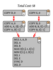
Figure 8: A partition graph of the greedy merge of the graph in Fig. 4.

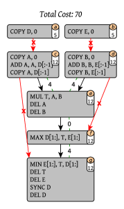
Figure 9: A partition graph of the unintrusive merge of the graph in Fig. 4.

V-D Optimal Partition Algorithm

Because the WSP problem is NP-hard, we cannot in general hope to solve it exactly in polynomial time. However, we may be able to solve the problems within reasonable time in common cases given a carefully chosen search strategy through the $2^{E}$ possible partitions. For this purpose, we have implemented a branch-and-bound algorithm, exploiting the monotonicity of the partition cost (Def. 6(2)). It is shown in Fig. 11, and proceeds as follows:

Before starting, the largest unintrusive partition is found. This is the largest partition that we can ensure is included in an optimal partition. The blocks of the unintrusive partition will be the vertices in our initial partition graph. Second, a good suboptimal solution is computed. We use the greedy algorithm for this purpose, but any scheme will do. We now start a search rooted in the $\top$-partition where everything is one block. This has the lowest cost, but will in general be illegal. Each recursion step cuts a weight edge that has not been considered before, if it yields a cost that is strictly lower than the currently best partition $G_{\min}$ (if the cost is higher than for $G_{\min}$, no further splitting will yield a better partition, and its search subtree can be ignored). If we reach a legal partition, this will be the new best candidate, and no further splitting will yield a better one. When the work queue is empty, $G_{\min}$ holds an optimal solution to WSP.

Fig. 11 shows the implementation, Fig. 10 shows an example of a branch-and-bound search tree, and Fig. 12 shows an optimal partition of the Python example with a partition cost of 38.

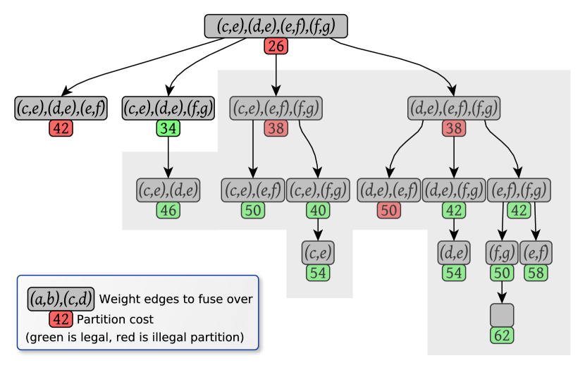
Figure 10: A branch-and-bound search tree of the unintrusively merged partition graph (Fig. 9). Each vertex lists a sequences of vertex merges that build a specific graph partition. The grayed out area indicates the part of the search tree that a depth-first-search can skip because of the cost bound.

Figure 11: The optimal merge algorithm that optimally merges the vertices in $G$. The function, $cost(G)$, returns the partition cost of the partition graph $G$.

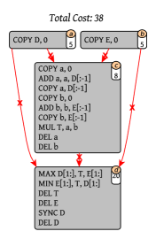
Figure 12: A partition graph of the optimal merge of the graph in Fig. 4.

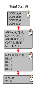
Figure 13: A partition graph of a Linear partition of the Python example (Fig. 3).

V-E Linear Merge

For completeness, we also implement a partition algorithm that does not use a graph representation. In this naïve approach, we simply go through the array operation list and add each array operation to the current partition block unless the array operations makes the current block illegal, in which case we add the array operation to a new partition block, which then becomes the current one. The asymptotic complexity of this algorithm is $\mathcal{O}\left(n^{2}\right)$ where $n$ is the number of array operations.

Fig. 13 show that result of partitioning the Python example with a cost of 58.

V-F Merge Cache

In order to amortize the execution time of applying the merge algorithms, Bohrium implements a merge cache of previously found partitions of array operation lists. It is often the case that scientific applications use large calculation loops such that an iteration in the loop corresponds to a list of array operations. Since the loop contains many iterations, the cache can amortize the overall execution time time.

VI Evaluation

In this section, we will evaluate the different partition algorithm both theoretically and practically. We execute a range of scientific Python benchmarks, which are part of an open source benchmark tool and suite named Benchpress.

Table I shows the specific benchmarks that we uses and Table II specifies the host machine. When reporting execution times, we use the results of the mean of 10 identical executions as well as error bars that shows two standard deviations from the mean.

We would like to point out that even though we are using benchmarks implemented in pure Python/NumPy, the performance is comparable to traditional high-performance languages such as C and Fortran. This is because Bohrium overloads NumPy array operations [7] in order to JIT compile and execute them in parallel seamlessly [12].

Benchmark	Input size (in 64bit floats)	Iterations
Black Scholes	$1.5{\mkern-2.0mu\times\mkern-2.0mu}10^{6}$	$20$
Game of Life	$10^{8}$	$20$
Heat Equation	$1.44{\mkern-2.0mu\times\mkern-2.0mu}10^{8}$	$20$
Leibnitz PI	$10^{8}$	$20$
Gauss Elimination	$2800$	$2799$
LU Factorization	$2800$	$2799$
Monte Carlo PI	$10^{8}$	$20$
27 Point Stencil	$4.2875{\mkern-2.0mu\times\mkern-2.0mu}10^{7}$	$20$
Shallow Water	$1.024{\mkern-2.0mu\times\mkern-2.0mu}10^{7}$	$20$
Rosenbrock	$2{\mkern-2.0mu\times\mkern-2.0mu}10^{8}$	$20$
Successive over-relaxation	$1.44{\mkern-2.0mu\times\mkern-2.0mu}10^{8}$	$20$
NBody	$6000$	$20$
NBody Nice	$40$ plantes, $2{\mkern-2.0mu\times\mkern-2.0mu}10^{6}$asteroids	$20$
Lattice Boltzmann D3Q19	$3.375{\mkern-2.0mu\times\mkern-2.0mu}10^{6}$	$20$
Water-Ice Simulation	$6.4{\mkern-2.0mu\times\mkern-2.0mu}10^{5}$	$20$

TABLE I: Benchmark applications

Processor:	Intel Core i7-3770
Clock:	3.4 GHz
#Cores:	4
Peak performance:	108.8 GFLOPS
L3 Cache:	16MB
Memory:	128GB DDR3
Operating system:	Ubuntu Linux 14.04.2 LTS
Software:	GCC v4.8.4, Python v2.7.6, NumPy 1.8.2

TABLE II: System specifications

Theoretical Partition Cost

Fig. 14 shows that theoretical partition cost (Def. 13) of the four different partition algorithms previously presented. Please note that the last five benchmarks do not show an optimal solution. This is because the associated search trees are too large for our branch-and-bound algorithm to solve. For example, the search tree of the Lattice Boltzmann is $2^{664}$, which is simply too large even if the bound can cut $99.999\%$ of the search tree away.

As expected, we observe that the three algorithms that do fusion, Linear, Greedy, and Optimal, have a significant smaller cost than the non-fusing algorithm Singleton. The difference between Linear and Greedy is significant in some of the benchmarks but the difference between greedy and optimal does almost not exist.

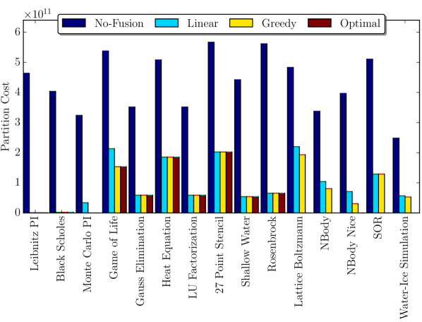
Figure 14: Theoretical cost of the different partition algorithms. NB: the last five benchmarks, Lattice Boltzmann, NBody, NBody Nice, SOR, Water-Ice Simulation, do not show an optimal solution.

Practical Execution Time

In order to evaluate the full picture, we do three execution time measurements: one with a warm fuse cache, one with a cold fuse cache, and one with no fuse cache. Fig. 15 shows the execution time when using a warm fuse cache thus we can compare the theoretical partition cost with the practical execution time without the overhead of running the partition algorithm. Looking at Fig. 14 and Fig. 15, it is evident that our cost model, which is a measurement of unique array accesses (Def. 13), compares well to the practical execution time result in this specific benchmark setup. However, there are some outliers – the Monte Carlo Pi benchmark has a theoretical partition cost of $1$ when using the Greedy and Optimal algorithm but has a significantly greater practical execution time. This is because the execution becomes computation bound rather than memory bound thus a further reduction in memory accesses does not improve performance. Similarly, in the 27 Point Stencil benchmark the theoretical partition cost is identical for Linear, Greedy, and Optimal, but in practice Optimal is marginally better. This is an artifact of our cost model, which define the cost of reads and writes identically.

With the cold fuse cache, the partition algorithm runs once in the first iteration of the computation. The results show that $20$ iterations, which most of the benchmarks uses, is enough to amortize the partition overhead (Fig. 16). Whereas, if we run with no fuse cache, i.e. we execute the partition algorithm in each iteration (Fig. 17), the Linear partition algorithm outperforms both the Greedy and Optimal algorithm because of its smaller time complexity.

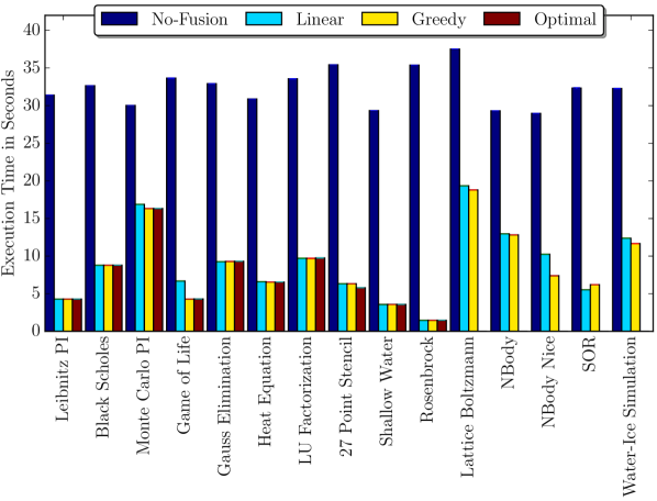
Figure 15: Execution time of the different partition algorithms using a warm cache.

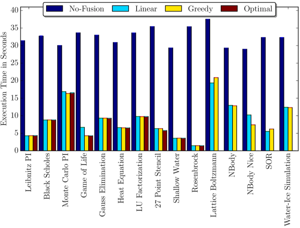
Figure 16: Execution time of the different partition algorithms using a cold cache.

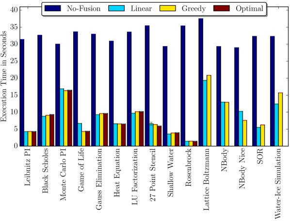
Figure 17: Execution time of the different partition algorithms using no cache.

VI-A Alternative Cost Model

With the theoretical and practical framework we are presenting in this paper, it is straightforward to explore the impact of alternative cost models. In this section, we will do exactly that – replace our cost model with alternative cost models and evaluate the effect on the execution time of the generated code.

Let us define and evaluate three alternative cost models, Max Contract, Max Locality, and Robinson, which are used in related literature [4, 13, 14]:

Definition 19.

The cost model Max Contract defines the cost of a partition, $P$, of array operations, $A$, as follows:

$$MaxContract(A,P)=|new[A]|-\sum_{B\in P}\mathbin{\scalebox{1.2}{$|$}}new[B]\cap del[B]\mathbin{\scalebox{1.2}{$|$}}$$ (5)

where $|new[A]|$ is the total number of allocated arrays. Thus, in this cost model, all arrays that are not contracted add $1$ to the cost.

Definition 20.

The cost model Max Locality defines the cost of a partition, $P$, of array operations, $A$, as follows:

$$MaxLocality(A,P)=\sum_{B\in P}\sum_{f\in B}\sum_{f^{\prime}\in(A\setminus B)}\mathbin{\scalebox{1.2}{$|$}}ext[f]\cap io[f^{\prime}]\mathbin{\scalebox{1.2}{$|$}}$$ (6)

In other words, this cost model penalizes each pair of array accesses not fused with a cost of $1$. NB: the cost is a pair-wise sum of all identical array accesses. Thus, fusing four identical array accesses achieves a cost saving of $6$ rather than $4$.

Definition 21.

The cost model Robinson defines the cost of a partition, $P$, of array operations, $A$, as follows:

$$Robinson(A,P) =\mathbin{\scalebox{1.2}{$|$}}P\mathbin{\scalebox{1.2}{$|$}}$$

$$+N\cdot MaxContract(A,P)$$

$$+N^{2}\cdot MaxLocality(A,P)$$ (7)

where $N$ is the total number of accessed arrays. In other words, this cost model combines Max Locality, Max Contract, and penalizes the number of partition blocks (in that priority). Furthermore, the size of $N$ guaranties that Max Locality always attach more importance than Max Contract which in turn always attach more importance than the number of partition blocks.

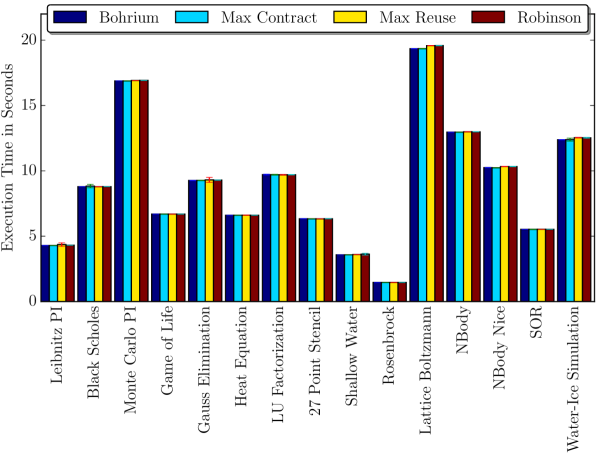
Figure 18: Execution time of the different cost models using the Linear partition algorithm and a warm cache.

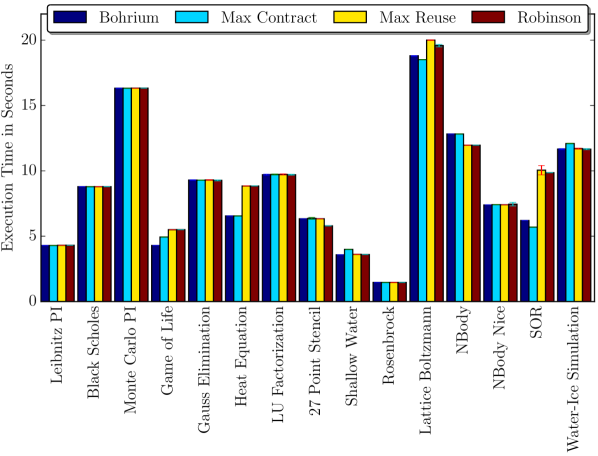
Figure 19: Execution time of the different cost models using the Greedy partition algorithm and a warm cache.

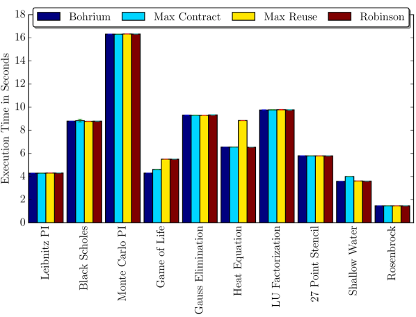
Figure 20: Execution time of the different cost models using the Optimal partition algorithm and a warm cache.

Fig. 18, 19, and 20 compares the execution time of the cost models using the Linear, Greedy, and Optimal partition algorithms respectively. The execution time of the Linear algorithm is more or less identical for all cost models.

The execution time of the Greedy algorithm shows some outliers – in the Heat Equation and the SOR benchmark, the performance of Max Locality and Robinson is significantly worse than the other two.

Finally, the execution time of the Optimal algorithm shows a case, Game of Life, where the Bohrium cost model performs better than the others. Additionally, in the Heat Equation benchmark the performance of Max Locality is significantly worse than the other three.

Overall, the practical performance of the four cost models is similar for the benchmarks presented. However, there are some important differences between them:

Since the objective of Max Contract is to maximize the number of array contractions exclusively, there exist programs where Max Contract is the only cost model that achieve this objective. With enough potential data locality in a program, the other three cost models will utilize this data locality at the expense of potential array contractions. This was a strong motivation for Darte and Huard [4] when they introduced an optimal solution to Max Contract. Fig. 21 shows a program fragment from [4] where Max Locality fails to maximize the number of array contractions. However, in this specific program fragment, both Bohrium and Robinson obtain the same solution as Max Contract because their objective includes the maximization of the number of array contractions.

⬇ A(1:N)=E(0:N-1) B = A*2 + 3 C = B + 99 D(1:N)=A(N:1:-1) + A(1:N) E = B + C*D F = E*4 + 2 G = E*8 - 3 H(1:N)=F(1:N)+G(1:N)*E(2:N+1)

(a)

⬇ DO I=1,N A(I) = E(I-1) ENDDO DO I=1,N b = A(I)*2 + 3 c = b + 99 d = A(N-I+1) + A(I) E(I) = b + c*d F(I) = E(I)*4 + 2 G(I) = E(I)*8 - 3 ENDDO DO I=1,N H(I) = F(I) + G(I)*E(I+1) ENDDO

(b)

⬇ DO I=1,N A(I) = E(I-1) ENDDO DO I=1,N b = A(I)*2 + 3 c = b + 99 d = A(N-I+1) + A(I) E(I) = b + c*d ENDDO DO I=1,N f = E(I)*4 + 2 g = E(I)*8 - 3 H(I) = f + g*E(I+1) ENDDO

(c)

Figure 21: A Fortran program fragment from [4], which is based on [13, 5]. (a) is an array operation version, (b) is the loop version that Max Locality will generate, and (c) is the loop version that Bohrium, Max Contract, and Robinson will generate.

VII Future Work

The cost models we present in this paper are abstract – they do not take the memory architecture of the execution hardware into account. Since the WSP formulation makes it easy to change the cost model, our future work is to develop cost models that, in detail, model architectures such as NUMA CPU, GPU, Intel Xeon Phi, and distributed shared-memory machines.

Furthermore, the only requirement to the cost model in the WSP formulation is that fusing two operations must be cost neutral or an advantage. Thus, it is perfectly legal to have cost models that reward fusion of specific operation types e.g. rewarding fusion of multiply and addition instructions to utilize the FMA instruction set available on recent Intel and AMD microprocessors.

VIII Conclusion

In this paper, we introduce the Weighted Subroutine Partition Problem (WSP), which unifies program transformations for fusion of loops, array operations, and combinators. Contrary to previous formulations of this problem, WSP incorporates the cost function into the formulation, which makes WSP able to handle a wide range of optimization objects. Furthermore, we show that the cost function must be part of the formulation to enable optimization objects that minimize data locality correctly.

We prove that WSP is NP-hard and implement a branch-and-bound algorithm that finds an optimal solution. Out of 15 application benchmarks, this branch-and-bound algorithm finds a solution for ten benchmarks within reasonable execution time.

We implement a greedy algorithm that finds a good solution to the WSP problem, works with any cost function, and is fast enough for Just-In-Time compilation (20 iterations is typically enough to amortize overhead).

To evaluate various WSP algorithms, we have incorporated the algorithms into Bohrium. The optimization objective is then to minimize data accesses through array contractions and data reuses within Just-In-Time compiled computation kernels.

As expected, our evaluation shows that minimizing data accesses have a significant performance impact. The 15 application benchmarks we evaluate in this paper experience a speedup ranging between 2 and 30, compared to no optimization.

However, our evaluation also shows that the various approaches to approximate or solve the WSP have only a marginal impact on the overall execution time of the benchmarks. Out of 15, only one benchmark performs significantly better using the optimal algorithm – approximately a speedup of 1.3 compared to the greedy algorithm. Similarly, the impact of various optimization objects is also minimal. This tells us that approximation algorithms will give us most of the savings, so more is won by making them faster than closer to optimal.

References

- [1] Michel Berkelaar, Kjell Eikland, and Peter Notebaert. lpsolve : Open source (Mixed-Integer) Linear Programming system.
- [2] B.L. Chamberlain, Sung-Eun Choi, C. Lewis, C. Lin, L. Snyder, and W.D. Weathersby. Zpl: a machine independent programming language for parallel computers. Software Engineering, IEEE Transactions on, 26(3):197–211, Mar 2000.
- [3] Elias Dahlhaus, David S Johnson, Christos H Papadimitriou, Paul D Seymour, and Mihalis Yannakakis. The complexity of multiway cuts. In Proceedings of the twenty-fourth annual ACM symposium on Theory of computing, pages 241–251. ACM, 1992.
- [4] Alain Darte and Guillaume Huard. New results on array contraction [memory optimization]. In Application-Specific Systems, Architectures and Processors, 2002. Proceedings. The IEEE International Conference on, pages 359–370. IEEE, 2002.
- [5] G. Gao, R. Olsen, V. Sarkar, and R. Thekkath. Collective loop fusion for array contraction. In Utpal Banerjee, David Gelernter, Alex Nicolau, and David Padua, editors, Languages and Compilers for Parallel Computing, volume 757 of Lecture Notes in Computer Science, pages 281–295. Springer Berlin Heidelberg, 1993.
- [6] Ken Kennedy and KathrynS. McKinley. Maximizing loop parallelism and improving data locality via loop fusion and distribution. In Languages and Compilers for Parallel Computing, volume 768 of Lecture Notes in Computer Science, pages 301–320. Springer Berlin Heidelberg, 1993.
- [7] Mads R. B. Kristensen, Simon A. F. Lund, Troels Blum, and Kenneth Skovhede. Separating NumPy API from Implementation. In 5th Workshop on Python for High Performance and Scientific Computing (PyHPC’14), 2014.
- [8] Mads R. B. Kristensen, Simon A. F. Lund, Troels Blum, Kenneth Skovhede, and Brian Vinter. Bohrium: Unmodified NumPy Code on CPU, GPU, and Cluster. In 4th Workshop on Python for High Performance and Scientific Computing (PyHPC’13), 2013.
- [9] Mads R. B. Kristensen, Simon A. F. Lund, Troels Blum, Kenneth Skovhede, and Brian Vinter. Bohrium: a Virtual Machine Approach to Portable Parallelism. In Parallel & Distributed Processing Symposium Workshops (IPDPSW), 2014 IEEE International, pages 312–321. IEEE, 2014.
- [10] E. Christopher Lewis, Calvin Lin, and Lawrence Snyder. The implementation and evaluation of fusion and contraction in array languages. In Proceedings of the ACM SIGPLAN 1998 Conference on Programming Language Design and Implementation, PLDI ’98, pages 50–59, New York, NY, USA, 1998. ACM.
- [11] D.B. Loveman. High performance fortran. Parallel & Distributed Technology: Systems & Applications, IEEE, 1(1):25–42, 1993.
- [12] Simon A. F. Lund and Brian Vinter. Automatic mapping of array operations to specific architectures. In submission to Elsevier journal on Parallel Computing, 2015. Ref. PARCO-D-15-00170.
- [13] Nimrod Megiddo and Vivek Sarkar. Optimal weighted loop fusion for parallel programs. In Proceedings of the ninth annual ACM symposium on Parallel algorithms and architectures, pages 282–291. ACM, 1997.
- [14] Amos Robinson, Ben Lippmeier, and Gabriele Keller. Fusing filters with integer linear programming. In Functional High Performance Computing 2014.
- [15] S. Van Der Walt, S.C. Colbert, and G. Varoquaux. The numpy array: a structure for efficient numerical computation. Computing in Science & Engineering, 13(2):22–30, 2011.
- [16] Thomas Wolle, Hans L Bodlaender, et al. A note on edge contraction. Technical report, Technical Report UU-CS-2004, 2004.