Perfect Sampling of Generalized Jackson Networks

Abstract.

We provide the first perfect sampling algorithm for a Generalized Jackson Network of FIFO queues under arbitrary topology and non-Markovian assumptions on the input of the network. We assume (in addition to stability) that the interarrival and service times of customers have finite moment generating function in a neighborhood of the origin, and the interarrival times have unbounded support.

1. Introduction

We present the first perfect sampling algorithm (i.e. unbiased sampling also known as exact simulation) for the steady-state of so-called Generalized Jackson Networks (GJNs).

A precise description of a GJN consists of $d$ single server queueing stations, with infinite capacity waiting rooms and each operating under a standard FIFO protocol. The $i$-th station receives arrivals from outside the network (i.e. external arrivals) according to a renewal process with arrival rate $\lambda_{i}\in[0,\infty)$ (note that $\lambda_{i}=0$ is possible, meaning that the $i$-th station does not receive external arrivals, but we assume that $\lambda_{i}>0$ for some $i\in\{1,...,d\}$). All the renewal arrival processes are independent. We use $\lambda=\left(\lambda_{1},...,\lambda_{d}\right)^{T}$ to denote the vector of arrival rates. (Throughout this paper all vectors are column vectors unless otherwise stated, and we use ^T to denote transposition.)

All the service requirements are independent. Inter-arrival times and service requirements are all independent. The mean service time at station $i$ is $1/\mu_{i}\in\left(0,\infty\right)$. We use $\mu=\left(\mu_{1},...,\mu_{d}\right)^{T}$ to denote the vector of service rates. The service requirements at station $i$ are i.i.d. (independent and identically distributed).

Immediately after a customer is served at the $i$-th station, he will go to station $j$ with probability $Q_{i,j}\in[0,1]$ for $j\in\{1,...,d\}$ and he will leave the network with probability $Q_{i,0}=1-\sum_{j=1}^{d}Q_{i,j}$. We write $Q=(Q_{i,j}:1\leq i,j\leq d)$ for the associated $d\times d$ substochastic routing matrix. The network is assumed to be open in the sense that $Q^{n}\rightarrow 0$ as $n\rightarrow\infty$. We assume, without the loss of generality, that $Q_{i,i}=0$. Otherwise we can redefine the service requirements via a geometric convolution with success probability equal to $1-Q_{i.i}$ and thus represent the network in terms of a model in which $Q_{i,i}=0$.

The so-called flow equations are given by

(1) $$\phi_{i}=\lambda_{i}+\sum_{j=1}^{d}Q_{j,i}\phi_{j},$$

which implies that $\phi=\left(\phi_{1},...,\phi_{d}\right)^{T}$ satisfies $\phi=\left(I-Q^{T}\right)^{-1}\lambda$. (Note that $\left(I-Q\right)^{-1}=I+Q+Q^{2}+....$ is well defined because the network is open.)

Under the previous setup, the GJN is stable (in the sense of possessing a steady-state distribution for the workload and queue length processes at each station) if and only if

(2) $$\phi<\mu,$$

where the inequality is understood componentwise.

Under mild assumptions (including for example the case of Poisson arrivals or phase-type inter-arrival and service times) we provide the first exact simulation algorithm for a Generalized Jackson Network. (The precise assumptions, listed as Assumptions 1-4, are given in Section 2.2.) All previous algorithms operate under more-restrictive assumptions relative to what is required in our algorithm. The more restrictive assumptions include: a) The networks are Markovian (i.e. inter-arrivals and service times are assumed to be exponential), or b) The networks are bounded (i.e. the stations are assumed to have rooms with finite buffer sizes); see, for example, [4] and [10].

The work of [1] is closest in spirit to our algorithm here. The authors in [1] consider a so-called stochastic fluid network (SFN), which is much simpler than a GJN because there is much less randomness in the system. Customers that arrive at station $i$ in a SFN bring service requirements which are i.i.d., this part is common to the GJN model. However, the workload is processed and transmitted to the stations in the network in the form of a fluid; so $Q_{i,j}$ represents the exact proportion of flow from station $i$ to $j$. Therefore, in particular, in a SFN there is no concept of queue-length. In addition, the SFNs treated in [1] has Poisson or Markov modulated arrivals and so even the arrival processes that we consider here are more general. We extend the algorithm in [1] in order to deal with arbitrary renewal processes (as opposed to only Poisson arrivals), the condition on Assumption 2 is needed to apply the technique of [1] based on a suitable exponential tilting (see also [6] and [2]), this connection to exponential changes of measure explains the need for Assumption 3.

The algorithm in [1] allows to obtain a sample from the maximum from time 0 to infinity, of a multidimensional random walk with negative drift. Here we extend the algorithm to sample from the running maximum (componentwise), that is, the maximum from time $n$ to infinity, for all $n\geq 0$. Our extension is given in Algorithm 4.

The real difficulty in doing perfect sampling of GJNs, however, arises from the fact that each customer might bring an arbitrarily long sequence of service requirements, because the description of the routing topology admits the possibility of visiting a given station multiple times. In addition, contrary to SFN’s, GJN’s are not monotone in their initial condition. This lack of monotonicity introduces challenges when applying standard perfect simulation techniques.

Our strategy is to apply Dominated Coupling From The Past (DCFTP), which requires the use of a suitable dominating process simulated backwards in time and in stationarity. We are able to use sample path comparison results developed by [5], which allow us to bound the total number of customers in the GJN by a set of suitably defined autonomous queues which are correlated. In addition, we provide additional sample path comparison results which are of independent interest (see Theorem 1).

We need to simulate, backwards in time, stationary and correlated autonomous queues. These processes can be represented, componentwise, in terms of an infinite horizon maximum of the difference of superposition of renewal processes (the difference having negative drift so the infinite horizon maximum is well defined). The fact that the queues are correlated comes from the fact that each jump in the renewal processes may correspond to a departure from one station, and at the same time, an arrival to another station due to the internal routing. We are able to extend the technique in [1] in order to deal with multidimensional and correlated renewal processes and thus complete the application of the DCFTP protocol.

The rest of the paper is organized as follows. In Section 2, we briefly discussing how DCFTP operates and describe the GJN. In Section 3, we construct a class of dominating processes which will be useful for our development. We provide a general overview of our algorithm and the main result of the paper in Section 4. Then we proceed by describing how to implement the subroutines of our algorithm in Section 5 and finish the paper with a numerical experiment in Section 6.

2. An introduction to DCFP and GJN

2.1. Elements of Dominated Coupling From The Past

Let us first provide a general description of DCFTP. Consider a stationary process $\left(Y\left(t\right):t\in\left(-\infty,\infty\right)\right)$, we are interested in sampling from $Y\left(0\right)$. Suppose that the following is available to the simulator:

• A pair of stochastic processes $\left(Y^{-}\left(t\right):t\in\left(-\infty,\infty\right)\right)$ and $\left(Y^{+}\left(t\right):t\in\left(-\infty,\infty\right)\right)$ coupled in such a way that $Y^{-}\left(t\right)\preccurlyeq Y\left(t\right)\preccurlyeq Y^{+}\left(t\right)$ for all $t$, where “$\preccurlyeq$” is any partial order.

• It is possible to simulate $\bar{\omega}:=\left(Y^{-}\left(t\right),Y^{+}\left(t\right):t\in[-T,0]\right)$ for a (finite almost surely) time $-T$ in the past such that: a)$\ Y^{+}\left(-T\right)=Y^{-}\left(-T\right)$, and b) $Y\left(0\right)$ can be obtained from the information used to generate $\bar{\omega}$.

A time $-T$ satisfying the conditions in DCFTP 2 is known as a coalescence time.

Generally, at least in the setting of Markov processes, the condition that $Y^{+}\left(-T\right)=Y^{-}\left(-T\right)$ combined with DCFTP 1 above indicates that the value of $Y\left(-T\right)$ is known and therefore at least the marginal evolution of $Y\left(\cdot\right)$ is completely determined, and so is the value of $Y(0)$. However, it is important to keep in mind that the processes $Y^{+},Y^{-}$ and $Y$ must remain coupled.

The validity of DCFTP is proved in [9]; the method is an extension of CFTP, which was proposed in the seminal paper of [11]. Intuitively, the idea is that if one could simulate the path $\left(Y^{-}\left(t\right),Y\left(t\right),Y^{+}\left(t\right):t\leq 0\right)$, from the infinite past, then one could obtain $Y\left(0\right)$ in stationality. However, since we can simulate $\bar{\omega}$ in finite time and use this information to reconstruct $Y\left(0\right)$, we do not need to simulate the process from the infinite past.

Obtaining the elements described in bullets DCFTP 1-2 above often requires several auxiliary constructions. In our particular application $Y\left(\cdot\right)$ corresponds to the number in system in each station (so $Y\left(\cdot\right)$ is a $d$-dimensional process) and we shall set $Y^{-}\left(t\right)=0$. The partial order relationship “$\preccurlyeq$” is based on the sum of the coordinates (i.e $x\preccurlyeq y$ if and only if $\sum x_{i}\leq\sum y_{i}$).

The process $Y^{+}\left(\cdot\right)$ is the one that will require auxiliary constructions, we shall first construct an auxiliary process $Y^{0}$ which dominates $Y$ based on artificially increasing (just slightly) the service requirement of all stations in the GJN. Then we will construct $Y^{+}$ which is a process similar to a GJN, except that the servers will enjoy vacation periods whenever there is no customer waiting in queue to be served. Finally, we will need an additional process, $Y^{\prime}$, which is corresponding to the autonomous queues and will allow us to identify the coalescence time $-T$.

2.2. Description of the GJN

In this section, we give detailed description and assumptions of the generalized Jackson network (GJN) we are going to simulate.

We consider a GJN consisting of $d$ service stations and each station has a single server. In the rest of our paper, we shall denote the GJN by $\mathcal{N}$. The basic assumptions of the GJN $\mathcal{N}$ is as follows: .

• Arrival times: Customers arrive (from the external world) at station $i$ according to some renewal process with i.i.d. interarrival times $U_{i}(n)$. In particular, $U_{i}(n)=A_{i}(n)-A_{i}(n-1)$ where $A_{i}\left(n\right)$ is the arrival time of the $n$-th customer of station $i$. The arrival rate $\lambda_{i}$ is defined as $E[U_{i}\left(k\right)]=1/\lambda_{i}\in(0,\infty]$. If $\lambda_{i}=0$ then $A_{i}\left(n\right)=\infty$. (By convention we let $\lambda_{i}U_{i}\left(1\right)=0$ if $\lambda_{i}=0$.)

• Service times: $\sigma_{i}(k)$ is the service time of the $k$-th customer that is served in station $i$. $\{\sigma_{i}(k)\}$ is a i.i.d. sequence and independent of the arrival times, routing indicators and service times of the other stations. The service rate $\mu_{i}$ is defined as $E[\sigma_{i}(k)]=1/\mu_{i}$.

• Routing mechanism: After finishing service, the $k$-th customer in station $i$ is assigned with a routing indicator $r_{i}\left(k\right)\in\{0,1,2,...,d\}$ and it will leave the network immediately if $r_{i}(k)=0$, or join the queue of station $r_{i}(k)$ otherwise. $\{r_{i}(k)\}$ is a i.i.d. sequence and independent of the arrival times, service times and routing indicators of the other stations. The routing probability $Q_{ij}$ is defined as $Q_{ij}=P(r_{i}(k)=j)$.

Clearly the sequences $\{A_{i}\left(n\right):n\geq 1\}$ together with $\{\left(r_{i}\left(k\right),\sigma_{i}\left(k\right)\right):k\geq 1\}$ for $i\in\{1,...,d\}$ are enough to fully describe the evolution of the queueing network, assuming that the initial state of the network is given. So, let us assume that the network is initially empty and let us write $Y_{i}\left(t\right)$ to denote the number of customers in the $i$-th service station at time $t$, including both in the queue and in service, for $i\in\{1,...,d\}$. As noted in the Introduction, the flow equations are given in equation (1), the vector $\phi_{i}$’s in $\phi=\left(\phi_{1},...,\phi_{d}\right)^{T}$ are called the net-input rates of the GJN.

In addition to the stability condition given in (2), throughout this paper we shall impose the following assumptions:

Assumptions:

1. The inter-arrival times have unbounded support. That is, if $\lambda_{i}>0$ then $P\left(U_{i}\left(1\right)>m\right)>0$ for all $m\in\left(0,\infty\right)$.

2. There exists $\delta>0$ such that for all $i$

   (3) $$\sup_{t\geq 0}E[\exp\left(\delta\lambda_{i}\left(U_{i}\left(1\right)-t\right)\right)|U_{i}\left(1\right) >t]<\infty,$$

   $$\sup_{t\geq 0}E[\exp\left(\delta\left(\sigma_{i}\left(1\right)-t\right)\right)|\sigma_{i}\left(1\right) >t]<\infty.$$

   In particular, $\lambda_{i}U_{i}\left(1\right)$ and $\sigma_{i}\left(1\right)$ have a finite moment generating function for all $i$.

3. The inter-arrival times and service times can be individually simulated exactly, and moreover, we can simulate from exponentially tiltings (i.e. the natural exponential family) associated to these distributions – see equation (10).

4. The inter-arrival times and service times have a continuous distribution.

Assumptions 1 to 4 are relatively mild and encompass a large class of models of interest including Poisson arrivals and phase-type service time distributions (and mixtures thereof). We shall also discuss immediate extensions to the case of Markov modulated GJNs. Assumption 1 ensure that the network will empty infinitely often with probability one. We require the existence of a finite moment generating function because we will apply an extension of a technique developed in [1], which is based on exponential tiltings and importance sampling, therefore the need for Assumption 3. We need the uniformity on exponential moments for conditional excess distributions in Assumption 2 because we apply a Lyapunov bound similar to that developed by [7]. However, we believe that this uniformity requirement is a technical condition and that our main result holds assuming only that (3) is satisfied for $t=0$. Finally, Assumption 4 is introduced for simplicity to avoid dealing with simultaneous events.

Under Assumptions 1 to 4 we provide an algorithm for sampling from the steady-state queue-length and workload processes at each station in the network. The number of random variables required to terminate our proposed procedure has a finite moment generating function in a neighborhood of the origin (in particular the expected termination time of the algorithm is finite).

3. Construction of the Auxiliary and Dominating Processes

In this section, we shall construct two dominating processes for $Y(t)$, related to vacation queues and autonomous queues.

3.1. An Auxiliary GJN

Before constructing the two bounding systems, we need to construct an auxiliary upper bound GJN, which we shall denote by $\mathcal{N}^{0}$. The auxiliary GJN $\mathcal{N}^{0}$, is obtained from the original GJN, $\mathcal{N}$, by slightly decreasing the service rates at each station while keeping the network stable. In particular, we shall select constants $a_{i}\geq 1$ for $i\in\{1,...,d\}$ momentarily. We define $\sigma_{i}^{0}\left(k\right)=\sigma_{i}\left(k\right)a_{i}$, and correspondingly set $\mu_{i}^{0}=\mu_{i}/a_{i}$ for $a_{i}\geq 1$ so that $\mu^{0}=\left(\mu_{1}^{0},...,\mu_{d}^{0}\right)^{T}$, satisfies,

(4) $$\lambda<\left(I-Q^{T}\right)\mu^{0},$$

componentwise. It is always possible to pick $a_{i}\geq 1$ satisfying (4). In order to see this, reason as follows. First, define $\mu^{0}=\left(I-Q^{T}\right)^{-1}\left(\lambda+\delta e\right)$ (where $e$ is the vector of ones and $\delta>0$ is to be chosen). Since $\phi=\left(I-Q^{T}\right)^{-1}\lambda<\mu$ and the matrix $\left(I-Q^{T}\right)^{-1}$ has non-negative elements, we can choose $\delta>0$ small enough so that $\mu_{i}>\mu_{i}^{0}$ and therefore $a_{i}=\mu_{i}/\mu_{i}^{0}>1$. Moreover, by definition

$$\left(I-Q^{T}\right)\mu^{0}=\lambda+\delta e>\lambda.$$

The evolution of $\mathcal{N}^{0}$, initially empty, is also fully described by the sequences $\{A_{i}\left(n\right):n\geq 1\}$ and $\{\left(r_{i}\left(k\right),\sigma_{i}^{0}\left(k\right)\right):k\geq 1\}$, $i\in\{1,...,d\}$, where $\sigma_{i}^{0}(k)=a_{i}\sigma_{i}(k)$. Let $Y_{i}^{0}\left(t\right)$ be the number of customers in the $i$-th service station at time $t$ (including both in queue and in service), for $i\in\{1,...,d\}$. As we shall review in Theorem 1, given the same initial condition at time 0, $\sum_{i}Y_{i}^{0}(t)\geq\sum_{i}Y_{i}(t)$, for all $t$ ; this is intuitive since every customer in $\mathcal{N}^{0}$ needs more service time at every station than in $\mathcal{N}$.

3.2. The Vacation System

We now describe the bonding system consisting of vacation queues, which we shall denote by $\mathcal{N}^{+}$. The system $\mathcal{N}^{+}$ evolves following almost the same rules as $\mathcal{N}^{0}$ except that, whenever the $i$-th server completes a service and no customer is waiting in queue to be served, the server enters a vacation period following the same distribution of $\sigma^{0}_{i}(k)$. The vacation periods are all independent, and also independent of the arrival times, service times and routing indicators. If at least one customer is waiting in queue, the server will work on the service requirement of the first customer waiting in queue.

In more detail, the vacation periods are not interrupted when a new customer arrives, instead the customer waits until the server finishes its current activity (current vacation or service). Moreover, if after completing a vacation the server still finds the queue empty, a new vacation period starts, and the server keeps taking vacation periods until, upon return of a vacation, the server finds at least one customer present in the queue, waiting to be served.

The evolution of the vacation system $\mathcal{N}^{+}$, coupled with $\mathcal{N}^{0}$, is fully described by the sequences $\{A_{i}\left(n\right):n\geq 1\}$ $\{\left(r_{i}\left(k\right),\sigma_{i}^{0}\left(k\right)\right):k\geq 1\}$, $i\in\{1,...,d\}$, along with the vacation period sequence $\left\{v_{i}^{0}\left(k\right):k\geq 1\right\}$. For each $i$, the sequence $\left\{\upsilon_{i}^{0}\left(k\right):k\geq 1\right\}$ is an i.i.d. copy of the sequence $\left\{\sigma_{i}^{0}\left(k\right):k\geq 1\right\}$. The random variable $\upsilon_{i}^{0}\left(k\right)$ denotes the $k$-th vacation period taken by the $i$-th server.

Let us write $Y_{i}^{+}\left(t\right)$ to denote the number of customers in the $i$-th station at time $t$ (including both in queue and in service). As stated in Theorem 1 below, we have that, given the same initial condition at time 0, $\sum_{i}Y_{i}^{+}(t)\geq\sum_{i}Y_{i}^{0}(t)$ for all $t$; this is intuitive since every customer in $\mathcal{N}^{+}$ keeps the same service time and routing (relative to $\mathcal{N}^{0}$), but the departure times must occur later due to the vacation periods.

3.3. The Autonomous System

The final bounding system is a set of the so-called autonomous queues which we shall denote by $\mathcal{N}^{\prime}$. In this subsection, we shall describe the evolution of this system and provide an expression for its number of customers in queue. In the next subsection, we shall explain how $\mathcal{N}^{\prime}$ is coupled with $\mathcal{N}^{+}$.

Define $\left(N_{i}\left(t\right):t\geq 0\right)$ to be the non-delayed renewal process corresponding to the sequence $\{A_{i}\left(n\right):n\geq 1\}$; that is, defining $A_{i}\left(0\right)=0$, by convention we have

$$N_{i}\left(t\right)=\max\{n\geq 0:A_{i}\left(n\right)\leq t\}.$$

Of course, $N_{i}\left(t\right)\equiv 0$ if $\lambda_{i}=0$.

We let $\left(V_{i}^{0}\left(k\right):k\geq 1\right)$ be a sequence of i.i.d. random variables with the same distribution $\sigma_{i}^{0}\left(k\right)$ (and therefore as $\upsilon_{i}^{0}\left(k\right)$). We write $B_{i}\left(0\right)=0$ and set $B_{i}\left(n\right)=V_{i}^{0}\left(1\right)+...+V_{i}^{0}\left(n\right)$. Then, define a renewal process

$$D_{i}\left(t\right)=\max\{n\geq 0:B_{i}\left(n\right)\leq t\}.$$

Moreover, for each $i\in\{1,...,d\}$ we define a sequence of i.i.d. random variables $(r_{i}^{\prime}\left(k\right):k\geq 1)$ such that

$$P\left(r_{i}^{\prime}\left(k\right)=j\right)=Q_{i,j},$$

for all $j\in\{0,1,...,d\}$. We then define

$$D_{i,j}\left(t\right)=\sum_{k=1}^{D_{i}\left(t\right)}I\left(r_{i}^{\prime}\left(k\right)=j\right)(\text{so that }D_{i}=\sum_{j=0}^{d}D_{i,j}).$$

The random variables $V_{i}^{0}\left(k\right)$’s and $r_{i}^{\prime}\left(k\right)$’s are all mutually independent and independent of the $A_{i}\left(k\right)$’s for all $i\in\{1,...,d\}$ and $k\geq 1$.

Let $Y_{i}^{\prime}\left(t\right)$ be the number of customers in the queue at the $i$-th station of $\mathcal{N}^{\prime}$. By the definition of autonomous queues, $Y_{i}^{\prime}\left(\cdot\right)$ evolves according to the following Stochastic Differential Equation

(5) $$\text{d}Y_{i}^{\prime}\left(t\right) =\text{d}N_{i}\left(t\right)+\sum_{j:j\neq i,1\leq j\leq d}\text{d}D_{j,i}\left(t\right)-I\left(Y_{i}^{\prime}\left(t_{-}\right)>0\right)\text{d}D_{i}\left(t\right),$$

$$Y_{i}^{\prime}\left(0\right) =0.$$

In simple words, the number of customers in queue at the $i$-th station increases when there is an external arrival (d$N_{i}\left(t\right)=1$) or an arrival (either virtual or true, see the explanation in Section 3.4) from any other station ($\sum_{j=0}^{d}$d$D_{j,i}\left(t\right)=1$), and it decreases at time $t$ after the completion of an activity (service or vacation, see the explanation is Section 3.4) only if the queue is not empty (i.e. $I\left(Y_{i}^{\prime}\left(t_{-}\right)>0\right)$ and d$D_{i}\left(t\right)=1$).

One nice property of $\mathcal{N}^{\prime}$ is that we have a convenient expression for $Y^{\prime}_{i}(t)$, which is essential for our CFTP algorithm to work. Let’s define

$$X_{i}\left(t\right)=N_{i}\left(t\right)+\sum_{j:j\neq i,1\leq j\leq d}D_{j,i}\left(t\right)-D_{i}\left(t\right),$$

recall that $Q_{i,i}=0$ so we have that $D_{i,i}\left(t\right)=0$, and thus we also can write $\sum_{j=1}^{d}D_{j,i}\left(t\right)$ in the previous display. Then, one can verify that the (unique) solution to equation (5) is given by (see for instance, [8])

$$Y_{i}^{\prime}\left(t\right)=X_{i}\left(t\right)-\min_{0\leq s\leq t}X_{i}\left(s\right)=\max_{0\leq s\leq t}\left(X_{i}\left(t\right)-X_{i}\left(s\right)\right).$$

3.4. Coupling between $\mathcal{N}^{\prime}$ and $\mathcal{N}^{+}$

In order to describe the coupling between $\mathcal{N}^{\prime}$ and $\mathcal{N}^{+}$, let us provide an interpretation of the SDE (5) describing $\mathcal{N}^{\prime}$. The evolution of the $i$-th queue in $\mathcal{N}^{\prime}$ can be seen as a single server queue with vacation periods. Customers arrive according to the superposition of the processes $N_{i}$ and $(D_{j,i}:1\leq j\leq d)$, the server takes a vacation whenever the queue is empty with a distribution which is identical to that of a generic service time. Arriving customers who find the queue empty must wait to be served only until the current vacation epoch finishes.

The difference between $\mathcal{N}^{\prime}$ and $\mathcal{N}^{+}$ is that in $\mathcal{N}^{+}$ no customers are “transferred” from station $i$ to $j$ at the end of a vacation epoch of server $i$. Note that these types of transfers actually might occur in $\mathcal{N}^{\prime}$ because it could be the case, for instance, that $Y_{i}^{\prime}\left(t-\right)=0$, $dD_{i}(t)=1$ and the corresponding $r_{i}^{\prime}(k)=j$ so that $dD_{i,j}(t)=1$ and a new customer joins the queue at station $j$. Consequently, in $\mathcal{N}^{\prime}$ there are two types of customers: a) true customers, as those in $\mathcal{N}^{+}$, which are the ones that correspond to external arrivals (i.e. arrivals from the processes $N_{i}$ for $i\in\{1,...,d\}$), and their corresponding routes through the network, and b) virtual customers, which does not exist in $\mathcal{N}^{+}$, are the ones generated by empty stations that transfer customers to other stations by the mechanism just described above. Therefore, to couple $\mathcal{N}^{\prime}$ and $\mathcal{N}^{+}$, we essentially need to distinguish between the true and virtual customers in $\mathcal{N}^{\prime}$.

Recall that the evolution of $\mathcal{N}^{\prime}$ is fully described by the process $N_{i}(\cdot)$, $D_{i}(\cdot)$ and $D_{ij}(\cdot)$, and $\mathcal{N}^{+}$ by the sequences $\{A_{i}(n)\}$, $\{r_{i}(k),\sigma_{i}^{0}(k)\}$ and $\{v_{i}(k)\}$. To describe the coupling of $\mathcal{N}^{\prime}$ and $\mathcal{N}^{+}$, we shall explain how to couple the pair of sequences. Roughly speaking, the two systems will share the same external arrivals, and each $V_{i}^{0}(k)$ (recall that $\{V_{i}^{0}(k)\}$ are the inter-renewal times of $D_{i}(\cdot)$) corresponds to a service time $\sigma_{i}(k^{\prime})$ when a customer is in service and to a vacation period $v_{i}(k^{\prime})$ otherwise. We provide the details next.

In our algorithm, we shall first simulate $\mathcal{N}^{\prime}$ on some finite time interval $[T_{1},T_{2}]$, the corresponding processes $N_{i}(t)$, $D_{i}(t)$ and $D_{ij}(t)$ on it, and sequences $\{A_{i}(n)\}$ and $\{(V_{i}(k),r_{i}^{\prime}(k)\}$. Then, the number of customers $Y_{i}^{+}(t)$ of the coupled vacation system $\mathcal{N}^{+}$ evolves according to the following SDE:

$$\text{d}\widehat{Y}_{i}^{+}\left(t\right) =\text{d}N_{0,i}\left(t\right)+\sum_{j:j\neq i,1\leq j\leq d}I(S_{j}^{+}\left(t_{-}\right)>0)\text{d}D_{j,i}\left(t\right)-I(\widehat{Y}_{i}^{+}\left(t_{-}\right)>0)\text{d}D_{i}\left(t\right),,$$

(6) $$\text{d}\widehat{S}_{i}^{+}\left(t\right) =(I(\widehat{Y}_{i}^{+}\left(t_{-}\right)>0)-I(S_{i}^{+}\left(t_{-}\right)>0))\text{d}D_{i}\left(t\right),$$

$$Y_{i}^{+}(t) =\widehat{Y}_{i}^{+}(t)+S_{i}^{+}(t).$$

Here $S_{i}^{+}(t)\in\{0,1\}$ is the number of customer in service at station $i$ at time $t$. In particular, we shall choose a special initial condition for $\mathcal{N^{+}}$ according to the comparison results that we shall explain in Section 3.5:

(7) $$\widehat{Y}_{i}^{+}\left(T_{1}\right)=Y_{i}^{\prime}(T_{1}),\text{ }S_{i}^{+}\left(T_{1}\right)=1.$$

The remaining service time of the customer at station $i$ is the residual jump time of $D_{i}(\cdot)$, i.e., $=B_{i}(D_{i}(T_{1})+1)-T_{1}$. Then, the sequences of $(\sigma_{i}^{0}\left(n\right)$, $r_{i}\left(n\right)$)_n≥1 can be extracted as follows.

Procedure 0: Coupling of $\mathcal{N}^{\prime}$ and $\mathcal{N}^{+}$:

1. Input $N_{i}(t)$, $D_{i}(t)$ and $D_{i,j}(t)$ for $1\leq i,j\leq d$ and $t\in[T_{1},T_{2}]$. Set $t_{i}=T_{1}$, $k^{s}_{i}=0$, $k^{v}_{i}=0$, and $n_{i}=1$.

2. Compute $Y^{+}(t)$ and $S^{+}(t)$ according to (3.4) and the initial condition (7).

3. For each $i$, while $t_{i}<T_{2}$, repeat the following:

   • $t_{i}\leftarrow t_{i}+V^{0}_{i}(n)$;

   • If $S_{i}^{+}(t_{i}-)=1$, update $k^{s}_{i}\leftarrow k^{s}_{i}+1$ and set $\sigma_{i}^{0}(k^{s}_{i})=V^{0}_{i}(n_{i})$ and $r_{i}(k^{s}_{i})=r_{i}^{\prime}(n_{i})$. Otherwise, update $k^{v}_{i}\leftarrow k^{v}_{i}+1$ and set $v_{i}(k^{v}_{i})=V^{0}_{i}(n_{i})$.

   • $n_{i}\leftarrow n_{i}+1$.

Lemma 1.

The extracted $(\sigma_{i}^{0}(k),r_{i}(k))$ form an i.i.d. sequence and independent of the sequence $\{A_{i}(n)\}$.

Proof.

This follows from the strong Markov property of the forward recurrence time processes of the renewal processes $N_{i}(\cdot)$, $D_{i}(\cdot)$ and $D_{ij}(\cdot)$. ∎

3.5. Comparison Results and Domination

Now we have a full description of the three systems $\mathcal{N}^{0}$, $\mathcal{N}^{+}$ and $\mathcal{N}^{\prime}$ that are coupled with the original GJN $\mathcal{N}$, and their corresponding queue length processes. The following theorem gives the comparison results among the four systems, which are essential in our DCFTP algorithm. Its proof is given in the Appendix.

Theorem 1.

Suppose that the networks $\mathcal{N}$, $\mathcal{N}^{0}$, $\mathcal{N}^{+}$, and $\mathcal{N}^{\prime}$ are all initially empty and are coupled as described through Section 4.1 to 4.4, then the following holds:

i) For any $t>0$,

$$\sum_{i=1}^{d}Y_{i}(t)\leq\sum_{i=1}^{d}Y_{i}^{0}(t)\leq\sum_{i=1}^{d}Y_{i}^{+}(t).$$

ii) Moreover, for any $t>0$, when $Y_{i}^{\prime}(t)=y_{i}$, then the service station $i$ in system $\mathcal{N}^{+}$ must satisfy $Y_{i}^{+}(t)\leq y_{i}+1$ and $S_{i}^{+}(t)\in\{0,1\}$.

iii) The network $\mathcal{N}^{+}$, driven by the SDE (3.4), is monotone in the initial condition. In other words, $y_{i}\in\{0,1,...\}$ and if $Y^{++},$ $Y^{+},$ $Y^{+-}$ satisfy the SDEs (3.4) with initial conditions $\widehat{Y}_{i}^{++}\left(0\right)=y_{i}+1$, $\widehat{S}_{i}^{++}\left(0\right)=1$; $\widehat{Y}_{i}^{+}\left(0\right)\leq y_{i}$, $\widehat{S}_{i}^{+}\left(0\right)\in\{0,1\}$, and $\widehat{Y}_{i}^{+}\left(0\right)=0=\widehat{S}_{i}^{+}\left(0\right)$, then $Y_{i}^{++}(t)\geq Y_{i}^{+}(t)\geq Y_{i}^{+-}(t)$ for all $t\geq 0$.

In the next section we explain how to use the previous result order to sample from the stationary distribution of $\mathcal{N}$, i.e. the joint distribution of customer numbers at each station, the remaining service requirement of the customers in service, and the remaining times to the next external arrivals to each station in steady state.

4. Our Algorithm and Main Result

Given the comparison results Theorem 1, we are now ready to given the main procedure of our DCFTP algorithm. In the rest of the paper, for any ergodic stochastic process $X(\cdot)$, we shall denote by $\bar{X}(\cdot)$ its two-sided stationary version.

Main Procedure:

1. Choose a constant $C_{T}>0$. Initialize $T\longleftarrow 0$.

2. Simulate the system $\mathcal{N}^{\prime}$ in steady state and backwards in time from $-T$ until $-T-C_{T}$. Obtain the corresponding processes $\bar{N}_{i}(\cdot)$, $\bar{D}_{i}(\cdot)$, $\bar{D}_{ij}(\cdot)$ and $\bar{Y}^{\prime}(\cdot)$ from $-T$ to $-T-C_{T}$. Update $T\longleftarrow T+C_{T}$.

3. Initialize a vacation system $\mathcal{N}^{++}$ at time $-T$ with $Y_{i}^{++}(-T)=\bar{Y}_{i}^{\prime}(-T)+1$, all servers occupied ($S_{i}^{+}(-T)=1$) , and the corresponding remaining service time equals to the time from $-T$ to the next jump time of process $\bar{D}_{i}(\cdot)$.

4. Compute $(Y_{i}^{++}(0):0\leq s\leq T)$, forward in time according to (3.4) in Section 3.4 and compute the corresponding sequences $\{A_{i}(n)\}$, $\{r_{i}(k),\sigma^{0}_{i}(k)\}$ and $\{v^{0}_{i}(k)\}$ according to Procedure 0.

5. If there exists $\tau\in[0,T]$ such that $Y_{i}^{++}(\tau)=0$ for all $i$, then we simulate a GJN $\mathcal{N}$ forward starting from $\tau<0$ to time $0$ with $Y_{i}(\tau)=0$ for all $i$ and driven by the sequence $\{A_{i}(n)\}$ and $\{r_{i}(k),\sigma_{i}(k)\}$ where each $\sigma_{i}(k)=\sigma^{0}_{i}(k)/a_{i}$. Output $Y_{i}(0)$ and terminate.

6. Otherwise, (if $Y^{+}(t)\neq 0$ for $t\in[0,T]$), go back to Step 2.

The above procedure can be validated by the following heuristic. Suppose $\bar{N}^{+}$ is the stationary vacation system coupled with $\bar{N}^{\prime}$. Then, according to Part ii) and iii) of Theorem 1, its queue length process $\bar{Y}_{i}^{+}(t)\leq Y_{i}^{++}(t)$ for all $i$ and $t\in[-T,0]$. Therefore, we can conclude that $\bar{Y}_{i}(\tau)=0$ for all $i$ and hence the coupled stationary GJN $\mathcal{N}$ must be empty at time $\tau$ by Part i) of Theorem 1. Then, we can recover the value of the stationary process $\bar{Y}_{i}(t)$ for $t\in[\tau,0]$ and the output $\bar{Y}_{i}(0)$ follows the steady-state distribution.

Theorem 2.

The state of the network given by the Main Procedure, including $Y\left(0\right)$ and the remaining service times at each station, follow the stationary distribution of the target GJN. Moreover, let $N$ be the total number of random variables to terminate the Main Procedure, then there is $\delta>0$ such that $E\exp\left(\delta N\right)<\infty$.

Step 3 through Step 5 in the Main Procedure can be done according to the coupling mechanism described in Section 3.1, 3.2, 3.4, and in particular, Procedure 0. The most difficult part is the execution of Step 2 and we shall explain this in Section 5. The proof, which is given at the end of Algorithm 4, in Section 7.2, mainly constitutes a recapitulation of our development.

5. Execution of Step 2 in Main Procedure: Stationary Construction and Backward Simulation of $\mathcal{\bar{N}}^{\prime}$

This section is devoted to explain how to execute Step 2 in Main Procedure, that is, to simulate a stationary version of $Y^{\prime}$ backwards in time. We shall explain this simulation procedure in three steps. In Section 5.1, we show a stationary version of $Y^{\prime}$ can be expressed by a multi-dimensional point process and its maximum. Then, we show the to simulate the point process and its maximum can be reduced to simulating several random walks jointly with their maximum. In the end, in Section 5.3, we explain how to simulate the random walks and their maximum, following the ideas in [1].

5.1. Express $Y^{\prime}$ by Point Processes

For each $i$, we define $\bar{N}_{0,i}\left(\cdot\right)$ as a two-sided, time stationary, renewal point process with inter-arrival time distribution being i.i.d. copies of $A_{i}\left(n+1\right)-A_{i}\left(n\right)$. We write $\{\bar{A}_{i}\left(n\right):n\in\mathbb{N}_{0}\mathbb{\cup(-N)\}}$ for the arrival times associated to $\bar{N}_{0,i}\left(\cdot\right)$, so that $\bar{A}\left(-1\right)<0<\bar{A}\left(0\right)<\bar{A}\left(1\right)$ and define

$$\bar{N}_{0,i}\left([a,b]\right)=\sum_{n}I\left(\bar{A}\left(n\right)\in[a,b]\right),$$

for any $a,b\in\left(-\infty,\infty\right)$.

Similarly, we let $\bar{D}_{i}\left(\cdot\right)$ to be a two-sided, time-stationary version of $D_{i}\left(\cdot\right)$ and write $\{\bar{B}_{i}\left(n\right):n\in\mathbb{N}_{0}\mathbb{\cup(-N)\}}$ for the arrival times associated to $\bar{D}_{i}\left(\cdot\right)$ also in increasing order and so that $\bar{D}_{i}\left(-1\right)<0<\bar{D}_{i}\left(0\right)<\bar{D}_{i}\left(1\right)$. As before,

$$\bar{D}_{i}\left([a,b]\right)=\sum_{n}I\left(\bar{B}_{i}\left(n\right)\in[a,b]\right).$$

Each $\bar{B}_{i}\left(n\right)$ is attached to a mark $\bar{r}_{i}^{\prime}\left(n\right)$ which are i.i.d. copies of the $r_{i}^{\prime}\left(n\right)$’s. All the $\bar{A}_{i}\left(n\right)$’s, the $\bar{D}_{i}\left(n\right)$’s, and the $r_{i}^{\prime}\left(n\right)$’s are mutually independent. Finally, for any $a,b\in(-\infty,\infty)$, define

$$\bar{D}_{i,j}\left([a,b]\right)=\sum_{n}I\left(\bar{B}_{i}\left(n\right)\in[a,b],\bar{r}_{i}^{\prime}\left(n\right)=j\right).$$

Intuitively, $N_{0,i}(\cdot)$ describes the external arrivals to station $i$, $D_{i,0}(\cdot)$ describes the potential departures from station $i$, and $D_{ij}(\cdot)$ describes the potential internal routings from station $i$ to $j$. For all $t\geq 0$, we define

(8) $$\bar{N}_{0,i}\left(t\right) =\bar{N}_{0,i}\left([0,t]\right),\text{ }\bar{N}_{0,i}\left(-t\right)=-\bar{N}_{0,i}\left([-t,0)\right),$$

$$\bar{D}_{i}\left(t\right) =\bar{D}_{i}\left([0,t]\right),\text{ }\bar{D}_{i}\left(-t\right)=-\bar{D}_{i}\left([-t,0)\right),$$

$$\bar{D}_{i,j}\left(t\right) =\bar{D}_{i,j}\left([0,t]\right),\text{ }\bar{D}_{i,j}\left(-t\right)=-\bar{D}_{i,j}\left([-t,0)\right).$$

and

$$\bar{X}_{i}\left(t\right)=\bar{N}_{0,i}\left(t\right)+\sum_{j:j\neq i,1\leq j\leq d}\bar{D}_{j,i}\left(t\right)-\bar{D}_{i}\left(t\right).$$

Then, $\bar{X}_{i}\left(t\right)$ is a two-sided stationary process. Finally put for $t\leq 0$,

(9) $$\bar{Y}^{\prime}(-t)=-\bar{X}(t)+\sup_{s\geq t}\bar{X}(s).$$

Observe that the for any deterministic time $T<0$, the process process $\{\bar{Y}_{i}^{\prime}\left(T+t\right)-\bar{Y}_{i}^{\prime}\left(T\right):0\leq t\leq\left|T\right|\}$ satisfies the SDE (5) only replacing the renewal processes with their respective stationary versions. We just need to show that $Y^{\prime}$ has a unique stationary distribution which is the same as the distribution of $\bar{Y}^{\prime}\left(0\right)$ and thus we have that $\bar{Y}^{\prime}$ is the time-reversed, stationary version of $Y^{\prime}$.

Lemma 2.

The autonomous queue $Y^{\prime}(\cdot)$ has a unique stationary distribution and therefore $\{\bar{Y}^{\prime}(-t):t\geq 0\}$ given by (9) is the time-reversed, stationary version of $Y^{\prime}$.

Proof of Lemma 2: We proceed with a construction procedure similar to the Loynes method. For $t\in[0,T]$ and any $y\in\mathbb{R}^{d}$ define

$$\text{d}Y_{i}^{\prime}\left(t\right) =\text{d}N_{0,i}\left(t\right)+\sum_{j:j\neq i,1\leq j\leq d}\text{d}D_{j,i}\left(t\right)-I\left(Y_{i}^{\prime}\left(t_{-}\right)>0\right)\text{d}D_{i}\left(t\right),$$

$$Y_{i}^{\prime}\left(0\right) =y.$$

We then have that

$$Y_{i}^{\prime}(t)=(y_{i}+X_{i}(t))-\inf_{0\leq s\leq t}\min(y_{i}+X_{i}(s),0)$$

and therefore

$$Y_{i}^{\prime}(T) =X_{i}(T)-\inf_{0\leq s\leq T}\min(X_{i}(s),-y_{i})$$

$$=-\inf_{0\leq s\leq T}\{\min(X_{i}(s),-y_{i})-X_{i}\left(T\right)\}$$

$$=\sup_{0\leq s\leq T}\{\max(X_{i}\left(T\right)-X_{i}\left(s\right),y_{i}+X_{i}\left(T\right))\}$$

$$=\sup_{0\leq u\leq T}\{\max(X_{i}\left(T\right)-X_{i}\left(T-u\right),y_{i}+X_{i}\left(T\right))\}.$$

As $T\rightarrow\infty$ we have that $X_{i}\left(T\right)\rightarrow-\infty$ and $X_{i}\left(T\right)-X_{i}\left(T-u\right)\Rightarrow$ $\bar{X}_{i}\left(u\right)$ as $T\rightarrow\infty$ (weakly) and therefore $Y_{i}^{\prime}(T)\Rightarrow\bar{Y}_{i}^{\prime}\left(0\right)$ regardless of the initial condition. $\Box$

Given the time-reversed, stationary version of $Y^{\prime}$, it suffices to simulate

$$\bar{X}_{i}^{\ast}\left(t\right)=\sup_{r\geq t}\bar{X}_{i}\left(r\right),$$

jointly with $\bar{X}_{i}\left(t\right)$ for all $i\in\{1,...,d\}$.

5.2. Connection between $\bar{X}_{i}^{\ast}\left(t\right)$ and Associated Random Walks

We note that $E[\bar{X}_{i}(1)]<1$ due to (4), therefore, $\bar{X}_{i}\left(t\right)\rightarrow-\infty$ as $t\rightarrow\infty$. Note that

$$X_{i}^{\ast}\left(t\right)=\max(\sup\{X_{i}\left(r\right):t\leq r\leq u\},X_{i}^{\ast}\left(u\right)).$$

To construct a bound for $\bar{X}^{*}_{i}(\cdot)$, we will construct a non-increasing process $Z_{i}\left(\cdot\right)$, such that $Z_{i}\left(u\right)\geq$ $X_{i}^{\ast}\left(u\right)$ and $Z_{i}\left(u\right)\rightarrow-\infty$ with probability one. Since $\sup\{X_{i}\left(r\right):t\leq r\leq u\}$ is clearly non-decreasing in $u$, our ability to simulate $Z_{i}\left(u\right)$ will allow us to sample $X^{\ast}\left(t\right)$ in finite time.

5.2.1. Construction of the Upper Bound $Z_{i}\left(\cdot\right)$

We now give the definition of $Z_{i}\left(\cdot\right)$. Following (4), we can pick $\bar{\delta}>0$ small enough so that

$$\lambda_{i}+\sum_{j=1}^{d}Q_{j,i}\mu_{j}^{0}+\bar{\delta}\left(1+\sum_{j=1}^{d}Q_{j,i}\right)<\mu_{i}^{0}.$$

Next we define $\gamma_{i}=\lambda_{i}+\bar{\delta}$, $\varphi_{j,i}=Q_{j,i}(\mu_{j}+\bar{\delta})$ and $\beta_{i}=\gamma_{i}+\sum_{j=1}^{d}\varphi_{j,i}$, and split

$$\bar{X}_{i}\left(t\right)=\left(\bar{N}_{0,i}\left(t\right)-\gamma_{i}t\right)+\sum_{j=1}^{d}\left(\bar{D}_{j,i}\left(t\right)-\varphi_{j,i}t\right)+(\beta_{i}t-\bar{D}_{i}\left(t\right))$$

so that

$$\bar{X}_{i}^{\ast}\left(t\right)\leq\sup_{r\geq t}\left(\bar{N}_{0,i}\left(t\right)-\gamma_{i}t\right)+\sum_{j=1}^{d}\sup_{r\geq t}\left(\bar{D}_{j,i}\left(t\right)-\varphi_{j,i}t\right)+\sup_{r\geq t}(\beta_{i}t-\bar{D}_{i}\left(t\right)).$$

Finally, we define three non-increasing processes as

$$\bar{N}_{0,i}^{\ast}\left(t\right) =\sup_{r\geq t}\left(\bar{N}_{0,i}\left(r\right)-\gamma_{i}r\right),$$

$$\bar{D}_{j,i}^{\ast}\left(t\right) =\sup_{r\geq t}\left(\bar{D}_{j,i}\left(r\right)-\varphi_{j,i}r\right),$$

$$\bar{D}_{i}^{\ast}\left(t\right) =\sup_{r\geq t}(\beta_{i}r-\bar{D}_{i}\left(r\right)),$$

for all $t\geq 0$. Observe that by the selection of $\beta_{i}$, $\varphi_{j,i}$, and $\gamma_{i}$, all the three processes just defined are non-increasing and go to minus infinity with probability 1. As a result,

$$Z_{i}\left(t\right):=\bar{N}_{0,i}^{\ast}\left(t\right)+\sum_{j=1}^{d}\bar{D}_{j,i}^{\ast}\left(t\right)+\bar{D}_{i}^{\ast}\left(t\right)\text{ is non-increasing and goes to }-\infty\text{ as }t\to\infty.$$

Now we explain how to simulate jointly

$$(\bar{N}_{0,i}^{\ast}\left(t\right),\bar{N}_{0,i}\left(t\right),\bar{D}_{j,i}^{\ast}\left(t\right),\bar{D}_{j,i}\left(t\right),\bar{D}_{i}^{\ast}\left(t\right),\bar{D}_{i}\left(t\right):i,j\in\{1,...,d\}).$$

5.2.2. Transforming the Simulation of $(Z\left(t\right):t\geq 0)$ into that of the Maximum of a Multidimensional Random Walk

Note that $\bar{N}_{0i}(\cdot)$ is piecewise linear with jumps, therefore it reaches its maximum only at (or right before) the times $\{\bar{A}_{i}(n)\}$ when it jumps. So are $D_{i}(\cdot)$ and $D_{ij}(\cdot)$. These results are formalized by the following lemma:

Lemma 3.

For $t\geq 0$ and assuming that $Q_{i,j}>0$ in the case of $\bar{D}_{j,i}^{\ast}\left(t\right)$, we have that

$$\bar{N}_{0,i}^{\ast}\left(t\right) =\max\left(\bar{N}_{0,i}(t)-\gamma_{i}t,\sup_{n>\bar{N}_{0,i}\left(t\right)}\left(n-\gamma_{i}\bar{A}_{i}\left(n\right)\right)+1\right),$$

$$\bar{D}_{i}^{\ast}\left(t\right) =\sup_{n>\bar{D}_{i}(t)}\Big{(}\beta_{i}\bar{B}_{i}\left(n\right)-n\Big{)},$$

$$\bar{D}_{j,i}^{\ast}\left(t\right) =\max\left(\bar{D}_{j,i}\left(t\right)-\varphi_{j,i}t,\sup_{n>\bar{D}_{j}(t)}\left(\sum_{k=1}^{n}I(r_{j}^{\prime}\left(k\right)=i)-\varphi_{j,i}\bar{B}_{j}\left(n\right)\right)+1\right).$$

Proof of Lemma 3: By definition, for any $r\geq 0$ such that $\bar{A}_{i}(k)\leq r<\bar{A}_{i}(k+1)$, $\bar{N}_{0,i}(r)=k+1$. As a result,

$$\max_{\bar{A}_{i}(k)\leq r<\bar{A}_{i}(k+1)}\left(\bar{N}_{0,i}(r)-\gamma_{i}r\right)=k+1-\bar{A}_{i}(k),$$

and the maximum is reached at $r=\bar{A}_{i}(k)$. As $\bar{A}_{i}(\bar{N}_{0,i}(t))\leq t<\bar{A}_{i}(\bar{N}_{0,i}(t)+1)$,

$$\bar{N}_{0,i}^{\ast}(t)=\sup_{r\geq t}(\bar{N}_{0,i}(r)-\gamma_{i}r)=\sup_{t\leq r<\bar{A}_{i}(\bar{N}_{0,i}(t)+1)}(\bar{N}_{0,i}(r)-\gamma_{i}r)\vee~{}\sup_{n>\bar{N}_{0,i}(t)}(n+1-\gamma_{i}\bar{A}_{i}(n)).$$

As

$$\sup_{t\leq r<\bar{A}_{i}(\bar{N}_{0,i}(t)+1)}(\bar{N}_{0,i}(r)-\gamma_{i}r)=\bar{N}_{0,i}(t)-\gamma_{i}t,$$

and

$$\sup_{n>\bar{N}_{0,i}(t)}(n+1-\gamma_{i}\bar{A}_{i}(n))=\sup_{n>\bar{N}_{0,i}\left(t\right)}\left(n-\gamma_{i}\bar{A}_{i}\left(n\right)\right)+1,$$

we have reach the expression for $\bar{N}_{0,i}^{\ast}(t)$. The same argument applies to $\bar{D}_{j,i}^{\ast}(\cdot)$. As to $\bar{D}_{i}^{\ast}(\cdot)$, note that

$$\sup_{\bar{B}_{i}(k)\leq r<\bar{B}_{i}(k+1)}(\beta_{i}r-\bar{D}_{i}(r))=\beta_{i}B_{i}(k+1)-(k+1)=\lim_{r\rightarrow\bar{B}_{i}(k+1)-}\beta_{i}r-\bar{D}_{i}(r),$$

and $\bar{B}_{i}(\bar{D}_{i}(t))\leq t<\bar{B}_{i}(\bar{D}_{i}(t)+1)$, therefore $\bar{D}_{i}^{\ast}(t)=\sup_{n>\bar{D}_{i}(t)}(\beta_{i}\bar{B}_{i}(n)-n)$. $\Box$

Therefore, to simulate the processes $\bar{N}^{*}_{0,i}(\cdot),\bar{D}^{*}_{i}(\cdot)$ and $\bar{D}^{*}_{ij}(\cdot)$, we only need to observe the processes $\bar{N}_{0,i}(\cdot),\bar{D}_{i}(\cdot)$ and $\bar{D}_{ij}(\cdot)$ at the discrete times when they jump, which can be expressed as random walks. The random walks have increments $(\bar{U}_{0,i}(n),\bar{V}_{i}^{0},\bar{V}^{0}_{ji}(0))$ defined as

$$\bar{U}_{0,i}\left(n\right) =1-\gamma_{i}(\bar{A}_{i}\left(n\right)-\bar{A}_{i}\left(n-1\right)),\text{ \ }\bar{V}_{i}^{0}\left(n\right)=\beta_{i}(\bar{B}_{i}\left(n\right)-\bar{B}_{i}\left(n-1\right))-1,$$

$$\bar{V}_{j,i}^{0}\left(n\right) =I(r_{j}^{\prime}\left(n\right)=i)-\varphi_{j,i}(\bar{B}_{j}\left(n\right)-\bar{B}_{j}\left(n-1\right)),\text{ for }n\geq 1$$

and for $n=0$,

$$\bar{U}_{i}\left(0\right)=-\gamma_{i}\bar{A}_{i}\left(0\right),\text{ \ \ }\bar{V}_{i}^{0}\left(0\right)=\beta_{i}\bar{B}_{i}\left(0\right),\text{ \ \ }\bar{V}_{j,i}^{0}\left(0\right)=-\varphi_{j,i}\bar{B}_{i}\left(0\right).$$

For the pair of $(i,j)$ with $\varphi_{j,i}=0$, we have that $\bar{V}_{j,i}^{0}\left(n\right)\equiv 0$ and we can ignore these coordinates. But in order to keep the notation succinct, let us denote by

$$\bar{W}_{i}\left(n\right)=(\bar{U}_{i}\left(n\right),\bar{V}_{i}^{0}\left(n\right),\bar{V}_{1,i}^{0}\left(n\right),...,\bar{V}_{d,i}^{0}\left(n\right))^{T}$$

for $n\geq 0$, and let

$$W\left(n\right)=(\bar{W}_{1}\left(n\right),\bar{W}_{2}\left(n\right),...,\bar{W}_{d}\left(n\right))^{T}.$$

Observe that $W\left(n\right)$ is a vector of dimension $d\times\left(d+2\right)$. To make the notation homogeneous we write $W_{j}\left(n\right)$ for the $j$-th coordinate of $W\left(n\right)$ where $1\leq j\leq d\times(d+2)$. Now we can define a $d\times\left(d+2\right)$-dimensional random walk $S\left(k\right)=S\left(k-1\right)+W\left(k\right)$, for $k\geq 1$, with $S\left(0\right)=W\left(0\right)$. Define its maximum process as

$$M_{j}\left(n\right)=\sup_{k\geq n}S_{j}\left(k\right)\text{ for }1\leq j\leq d\times(d+2).$$

Following Lemma 3, to simulate

$$(\bar{N}_{0,i}^{\ast}\left(t\right),\bar{N}_{0,i}\left(t\right),\bar{D}_{j,i}^{\ast}\left(t\right),\bar{D}_{j,i}\left(t\right),\bar{D}_{i}^{\ast}\left(t\right),\bar{D}_{i}\left(t\right):i,j\in\{1,...,d\})$$

is equivalent to simulate $\left(M\left(n\right),S\left(n\right):n\geq 0\right)$ jointly. Fortunately, there is an algorithm that allows us to carry out this simulation problem for $(M\left(n\right),S\left(n\right))$, adapted from work of [1] and [3], we provide details here for completeness.

Remark: In the following sections we shall simulate $(M\left(n\right)-W\left(0\right),S\left(n\right)-W\left(0\right))$, which is equivalent to simulating the sequence $\left(M\left(n\right),S\left(n\right):n\geq 0\right)$ assuming that $S\left(0\right)=0$. In the end, the random variable $W\left(0\right)$ can be simulated independently from everything else.

5.3. Sampling the Infinite Horizon Maximum of a Multidimensional Random Walk with Negative Drift

Let $S_{l^{\prime}}\left(n\right)$ be the coordinate of the random walk corresponding to $\bar{V}_{j,i}^{0}\left(n\right)$. We have that either $S_{l^{\prime}}\left(n\right)\equiv 0$ when $Q_{i,j}=0$, or $E[S_{l^{\prime}}\left(n\right)]<0$. For those coordinates for which $S_{l^{\prime}}\left(n\right)\equiv 0$ we have that $M_{l^{\prime}}\left(n\right)=0$ and there is nothing to do. So, let us assume for simplicity and without loss of generality that $E[S_{i}\left(n\right)]<0$ for all $1\leq i\leq l=d\left(d+2\right)$.

Define for each $\theta\in\mathbb{R}$

$$\psi_{i}\left(\theta\right)=\log E[\exp\left(\theta_{i}W_{i}\left(k\right)\right)],$$

and set

(10) $$P_{\theta_{i}}\left(W_{1}\left(k\right)\in dy_{1},...,W_{l}\left(k\right)\in dy_{l}\right)$$

$$=~{} \frac{\exp\left(\theta_{i}y_{i}-\psi_{i}\left(\theta\right)\right)}{E[\exp\left(\theta_{i}W_{i}\left(k\right)\right)]}P\left(W_{1}\left(k\right)\in dy_{1},...,W_{d}\left(k\right)\in dy_{d}\right),$$

where $\theta_{i}\in\mathbb{R}$ and $E\exp\left(\theta_{i}W_{i}\left(k\right)\right)<\infty$. Moreover, we impose the following assumption for simplicity.

Assumption 2b): For each $i$ there exists $\theta_{i}^{\ast}$ such that

$$\psi_{i}\left(\theta_{i}^{\ast}\right)=0.$$

Remark: Assumption 2b) is a strengthening of Assumption 2. We can carry out our ideas under Assumption 2 following [1] as we explain next. First, instead of ($M\left(n\right):n\geq 0)$, given a vector $a^{\prime}=\left(a_{1}^{\prime},a_{2}^{\prime},...,a_{d}^{\prime}\right)^{T}$ with non-negative components that we will explain how to choose momentarily, consider the process $S_{a^{\prime}}(\cdot)$ and $M_{a^{\prime}}\left(\cdot\right)$ defined by

$$S_{a^{\prime}}\left(n\right):=S\left(n\right)+a^{\prime}n,~{}M_{a^{\prime}}\left(n\right)=\max_{k\geq n}\left(S_{a}\left(k\right)\right).$$

Note that we can simulate $\left(S\left(n\right),M\left(n\right):n\geq 0\right)$ if we are able to simulate $\left(S_{a^{\prime}}\left(n\right),M_{a^{\prime}}\left(n\right):n\geq 0\right)$. Now, note that $\psi_{i}\left(\cdot\right)$ is strictly convex and that $d\psi_{i}\left(0\right)/d\theta<0$ so there exists $a_{i}^{\prime}>0$ large enough to force the existence of $\theta_{i}^{\ast}>0$ such that $E[\exp\left(\theta_{i}^{\ast}W_{i}\left(1\right)+a_{i}^{\prime}\theta_{i}^{\ast}\right)]=1$, but at the same time small enough to keep $E[\left(W_{i}\left(1\right)+a_{i}^{\prime}\right)]<0$; again, this follows by strict convexity of $\psi_{i}\left(\cdot\right)$ at the origin. So, if Assumption A3b) does not hold, but Assumption A3) holds, one can then execute Algorithm 2 based on the process $S_{a^{\prime}}(\cdot)$.

5.3.1. Construction of $\left(S\left(n\right),M\left(n\right):\,n\geq 0\right)$ via “milestone events”

We will describe the construction of a pair of sequences of stopping times (with respect to the filtration generated by $(S\left(n\right):n\geq 0)$), denoted by $(\Lambda_{n}:n\geq 0)$ and $(\Gamma_{n}:n\geq 1)$, which track certain downward and upward milestones in the evolution of $\left(S\left(n\right):\,n\geq 0\right)$. We follow similar steps as described in [2] and [3]. These “milestone events” will be used in the design of our proposed algorithm. The elements of the two stopping times sequences interlace with each other (when finite) and their precise description follows next.

We start by fixing any $m>0$. Eventually, we shall choose $m$ suitably large as we shall discuss in in equation (18), but our conceptual discussion here is applicable to any $m>0$. Now set $\Lambda_{0}=0$. We observe the evolution of the process $(S\left(n\right):\,n\geq 0)$ and detect the time $\Lambda_{1}$ (the first downward milestone),

$$\Lambda_{1}=\inf\left\{n\geq\Lambda_{0}:\,S(n)<-m\mathbf{e}\right\},$$

where the inequality is componentwise. That is, $S_{i}(n)<-m$ for all $1\leq i\leq l$.

Once $\Lambda_{1}$ is detected we check whether or not $\left\{S\left(n\right):\,n\geq\Lambda_{1}\right\}$ ever goes above the height $S\left(\Lambda_{1}\right)+m$ (the first upward milestone); namely we define

$$\Gamma_{1}=\inf\left\{n\geq\Lambda_{1}:\,S_{i}(n)>m+S_{i}\left(\Lambda_{1}\right)\text{ for some }1\leq i\leq l\right\}.$$

For now let us assume that we can check if $\Gamma_{1}=\infty$ or $\Gamma_{1}<\infty$ (how exactly to do so will be explained in Section 5.3.2). To continue simulating the rest of the path, namely $\left\{S\left(n\right):\,n>\Lambda_{1}\right\}$, we potentially need to keep track of the conditional upper bound implied by the fact that $\Gamma_{1}=\infty$. To this end, we introduce the conditional upper bound variable $C_{UB}$ (initially $C_{UB}=\infty$). If at time $\Lambda_{1}$ we detect that $\Gamma_{1}=\infty$, then we set $C_{UB}=S\left(\Lambda_{1}\right)+m$ and continue sampling the path of the random walk conditional on never crossing the upper bound $S\left(\Lambda_{1}\right)+m$ in any of the coordinates. That is, conditional on $\left\{S\left(n\right)<C_{UB}:\,n>\Lambda_{1}\right\}$. Otherwise, if $\Gamma_{1}<\infty$, we simulate the path conditional on $\Gamma_{1}<\infty$, until we detect the time $\Gamma_{1}$. We continue on, sequentially checking whenever a downward or an upward milestone is crossed as follows: for $j\geq 2$, define

(11) $$\begin{array}[c]{l}\Lambda_{j}=\inf\left\{n\geq\Gamma_{j-1}I\left(\Gamma_{j-1}<\infty\right)\vee\Lambda_{j-1}:\,S\left(n\right)<S\left(\Lambda_{j-1}\right)-m\mathbf{e}\right\}\\ \Gamma_{j}=\inf\left\{n\geq\Lambda_{j}:\,S_{i}\left(n\right)-S_{i}\left(\Lambda_{j}\right)>m\text{ for some }1\leq i\leq l\right\},\end{array}$$

with the convention that if $\Gamma_{j-1}=\infty$, then $\Gamma_{j-1}I\left(\Gamma_{j-1}<\infty\right)=0$. Therefore, we have that $\Gamma_{j-1}I\left(\Gamma_{j-1}<\infty\right)>\Lambda_{j-1}$ if and only if $\Gamma_{j-1}<\infty$.

Let us define

(12) $$\Delta=\inf\{\Lambda_{n}:\Gamma_{n}=\infty,n\geq 1\}.$$

So, for example, if $\Gamma_{1}=\infty$ we have that $\Delta=\Lambda_{1}$ and the drifted random walk will never reach level $S\left(\Lambda_{1}\right)+m<S(0)$ again. This allows us to evaluate $M\left(0\right)$ by computing

(13) $$M\left(0\right)=\max\left\{S\left(n\right):\,0\leq n\leq\Delta\right\},$$

the maximum is taken over $n$ for each coordinate.

Similarly, the event $\Gamma_{j}=\infty$, for some $j\geq 1$, implies that the level $S_{i}\left(\Lambda_{j}\right)+m$ is never crossed for any $i$ (that is $S_{i}\left(n\right)\leq S_{i}\left(\Lambda_{j}\right)+m$) for all $n\geq\Lambda_{j}$, and we let $C_{UB}=S\left(\Lambda_{j}\right)+m$. The value of the vector $C_{UB}$ keeps updating as the random walk evolves, at times where $\Gamma_{j}=\infty$.

The advantage of considering these stopping times is the following: once we observed that some $\Gamma_{j}=\infty$, the values of $\left\{M_{i}\left(n\right):\,n\leq\Gamma_{j-1}1(\Gamma_{j-1<\infty})\vee\Lambda_{j-1}\right\}$ for each $1\leq i\leq l$ are known without a need of further simulation. Proposition 1 ensures that it suffices to sequentially simulate $(\Lambda_{n}:n\geq 0)$ and $(\Gamma_{n}:n\geq 1)$ jointly with the underlying random walk in order to sample from the sequence $\left(S\left(n\right),\,M\left(n\right):\,n\geq 0\right)$. The proof of Proposition 1 is easily adapted from the one dimensional case discussed in [3] and thus it is omitted.

Proposition 1.

Set $\Lambda_{0}=0$ and let $(\Lambda_{n}:\,n\geq 1)$ and $(\Gamma_{n}:\,n\geq 1)$ be as (11). We have that

(14) $$\begin{array}[c]{cccc}P_{0}\left(\lim_{n\rightarrow\infty}\Lambda_{n}=\infty\right)=1&\text{ and }&P_{0}\left(\Lambda_{n}<\infty\right)=1,&\forall n\geq 1.\end{array}$$

Furthermore,

(15) $$P_{0}\left(\Gamma_{n}=\infty,\,\text{i.o.}\,\right)=1.$$

In the setting of Proposition 1, for each $k\geq 0$ we can define $N_{0}\left(k\right)=\inf\left\{n\geq 1:\,\Lambda_{n}\geq k\right\}$ and $\mathcal{T}\left(k\right)=\inf\left\{j\geq N_{0}\left(k\right)+1:\,\Gamma_{j}=\infty\right\}$. Both of them are finite random variables such that

(16) $$M\left(k\right)=\max\left\{S\left(n\right):\,k\leq n\leq\Lambda_{\mathcal{T}\left(k\right)}\right\}$$

In other words, $\Lambda_{\mathcal{T}\left(k\right)}$ is the time, not earlier than $k$, at which we detect a second unsuccessful attempt at building an upward patch directly. The fact that the relation in (16) holds, follows easily by construction of the stopping times in (11). Note that it is important, however, to define $\mathcal{T}\left(k\right)\geq N_{0}\left(k\right)+1$ so that $\Lambda_{N_{0}\left(k\right)+1}$ is computed first. In that way, we can make sure that the maximum of the sequence $\left(S\left(n\right):\,n\geq k\right)$ is achieved between $k$ and $\Lambda_{\mathcal{T}\left(k\right)}$.

These observation gives rise to our suggested high-level scheme. The procedure sequentially constructs the random walk in the intervals $\left[\Lambda_{n-1},\Lambda_{n}\right)$ for $n\geq 1$. Here is the high-level procedure to construct $\left(S\left(n\right),\,M\left(n\right):n\geq 0\right)$:

Algorithm 1.

At the $k$-th iteration, for $k\geq 1$:
Step 1: “downward patch”. Conditional on the path not crossing $C_{UB}$ we simulate the path until we detect $\Lambda_{k}\,$, which is the first time when the random walk visits the set $(-\infty,S_{1}(\Lambda_{k-1})-m]\times...\times(-\infty,S_{l}(\Lambda_{k-1})-m]$ .
Step 2: “upward patch”. Check whether or not the level $S_{i}(\Lambda_{k})+m$ is ever crossed by any of the coordinates $i$. That is, whether $\Gamma_{k}<\infty$ or not. If the answer is “Yes” then, conditional on the path crossing $S_{i}(\Lambda_{k})+m$ for some $i$, but not crossing the level $\left(C_{UB}\right)_{i}$, we simulate the path until we detect $\Gamma_{k}$, the first time the level $S_{i}(\Lambda_{k})+m$ for at least one of the coordinates $i$ . Otherwise $\left(\Gamma_{j}=\infty\right)$, and we can update $C_{UB}$: $C_{UB}\leftarrow S(\Lambda_{j})+m\mathbf{e}$

The implementation of the steps in Algorithm 1 will be discussed in detail in the next sections, culminating with the precise description given in Algorithm 4 at the end of Section 5.3.3.

5.3.2. Sampling $M\left(0\right)$ jointly with $\left(S\left(1\right),...,S\left(\Delta\right)\right)$

The goal of this section is to sample exactly from $M\left(0\right)$. To this end we need to simulate the sample path up to the first $\Gamma_{j}$ such that $\Gamma_{j}=\infty$ (recall that $\Delta$ was defined to be the corresponding $\Lambda_{j}$). This sample path will be used in the construction of further steps in Algorithm 1. This construction is directly taken from [1].

For any positive vectors $a,b>0$. Let

(17) $$\begin{array}[c]{lc}\tau_{b}=\inf\left\{n\geq 0:\,S_{i}\left(n\right)>b_{i}\text{ for some }i\right\},&\\ \tau_{-b}=\inf\left\{n\geq 0:\,S_{i}\left(n\right)<-b_{i}\text{ for all }i\right\},&\\ P_{a}\left(\cdot\right)=P\left(\cdot\,\mid S\left(0\right)=a\right).&\end{array}$$

Since we concentrate on $M\left(0\right)$, we have that $C_{UB}=\infty$. We first need to explain a procedure to generate a Bernoulli random variable with success parameter $P_{0}\left(\tau_{m\mathbf{e}}<\infty\right)$, for suitably chosen $m>0$. Also, this procedure, as we shall see, will allow us to simultaneously simulate $\left(S\left(1\right),...,S\left(\tau_{m\mathbf{e}}\right)\right)$ given that $\tau_{m\mathbf{e}}<\infty$.

We think of the probability measure $P_{0}\left(\cdot\right)$ as defined on the canonical space $\Omega=\{0\}\times\mathbb{R}^{l}\times\mathbb{R}^{l}\times...$ endowed with $\sigma$-field generated by the Borel $\sigma$-field of finite dimensional projections (i.e. the Kolmogorov $\sigma$-field). Our goal is to simulate from the conditional law of $(S\left(n\right):0\leq n\leq\tau_{m\mathbf{e}})$ given that $\tau_{m\mathbf{e}}<\infty$ and $S(0)=0$, which we shall denote by $P_{0}^{\ast}$ in the rest of this part.

First, we select $m>0$ such that

(18) $$\sum_{k=1}^{l}\exp\left(-\theta_{i}^{\ast}m\right)<1.$$

Now let us introduce our proposal distribution $P_{0}^{\prime}\left(\cdot\right)$, defined on the space $\Omega^{\prime}=\Omega\times\{1,2,...,l\}$. We endow the probability space with the associated Kolmogorov $\sigma$-field. So, a typical element $\omega^{\prime}$ sampled under $P_{0}^{\prime}\left(\cdot\right)$ is of the form $\omega^{\prime}$=(($S\left(n\right):n\geq 0$),$Index)$, where $Index\in\{1,2,...,l\}$. The distribution of $\omega^{\prime}$ induced by $P_{0}^{\prime}\left(\cdot\right)$ is described as follows, first,

(19) $$P_{0}^{\prime}\left(Index=i\right)=w_{i}:=\frac{\exp\left(-\theta_{i}^{\ast}m\right)}{\sum_{j=1}^{l}\exp\left(-\theta_{j}^{\ast}m\right)}.$$

Now, given $Index=i$, for every set $A\in\sigma$($S\left(k\right):0\leq k\leq n)$,

$$P_{0}^{\prime}\left(A|Index=i\right)=E_{0}[\exp\left(\theta_{i}^{\ast}Z_{i}\left(t\right)\right)I_{A}].$$

In particular, the Radon-Nikodym derivative (i.e. the likelihood ratio) between the distribution of $\omega=(S\left(k\right):0\leq k\leq n)$ under $P_{0}^{\prime}\left(\cdot\right)$ and $P_{0}\left(\cdot\right)$ is given by

$$\frac{dP_{0}^{\prime}}{dP_{0}}\left(\omega\right)=\sum_{i=1}^{l}w_{i}\exp\left(\theta_{i}^{\ast}S_{i}\left(n\right)\right).$$

The distribution of $(S\left(k\right):k\geq 0)$ under $P_{0}^{\prime}\left(\cdot\right)$ is precisely the proposal distribution that we shall use to apply acceptance / rejection. It is straightforward to simulate under $P_{0}^{\prime}\left(\cdot\right)$. First, sample $Index$ according to the distribution (19). Then, conditional on $Index=i$, the process $S\left(\cdot\right)$ is also a multidimensional random walk. Indeed, given $Index=i$, under $P_{0}^{\prime}\left(\cdot\right)$ it follows that $S\left(n\right)$ can be represented as

(20) $$S\left(n\right)=W^{\prime}\left(1\right)+...+W^{\prime}\left(n\right),$$

where $W^{\prime}\left(k\right)$’s are i.i.d. with distribution obtained by exponential titling, such that for all $A\in\sigma(W^{\prime}\left(k\right))$,

(21) $$P_{0}^{\prime}(W^{\prime}\left(k\right)\in A)=E[\exp(\theta_{i}^{\ast}W_{i})I_{A}].$$

Now, note that we can write

$$E_{0}^{\prime}\left(S_{Index}\left(n\right)\right) =\sum_{i=1}^{l}E_{0}(S_{i}(n)\exp\left(\theta_{i}^{\ast}S_{i}\left(n\right)\right))P_{0}^{\prime}\left(Index=i\right)$$

$$=\sum_{i=1}^{l}\frac{d\psi_{i}\left(\theta_{i}^{\ast}\right)}{d\theta}w_{i}>0,$$

where the last inequality follows by convexity of $\psi_{k}\left(\cdot\right)$ and by definition of $\theta_{k}^{\ast}$. So, we have that $S_{Index}\left(n\right)\nearrow\infty$ as $n\nearrow\infty$ with probability one under $P_{0}^{\prime}\left(\cdot\right)$, by the Law of Large Numbers. Consequently $\tau_{m\mathbf{e}}<\infty$ a.s. under $P_{0}^{\prime}\left(\cdot\right)$.

Recall that $P_{0}^{\ast}\left(\cdot\right)$ is the conditional law of $\left(S\left(n\right):0\leq n\leq\tau_{m\mathbf{e}}\right)$ given that $\tau_{m\mathbf{e}}<\infty$ and $S\left(0\right)=0$. In order to assure that we can indeed apply acceptance / rejection theory to simulate from $P_{0}^{\ast}(\cdot)$, we need to show that the likelihood ratio $dP_{0}/dP_{0}^{\prime}$ is bounded. Indeed,

$$\frac{dP_{0}^{\ast}}{dP_{0}^{\prime}}\left(S\left(n\right):0\leq t\leq\tau_{m\mathbf{e}}\right) =\frac{1}{P_{0}\left(\tau_{m\mathbf{e}}<\infty\right)}\times\frac{dP_{0}}{dP_{0}^{\prime}}\left(S\left(n\right):0\leq t\leq\tau_{m\mathbf{e}}\right)$$

(22) $$=\frac{1}{P_{0}\left(\tau_{m\mathbf{e}}<\infty\right)}\times\frac{1}{\sum_{i=1}^{l}w_{i}\exp\left(\theta_{i}^{\ast}S_{i}\left(\tau_{m\mathbf{e}}\right)\right)}.$$

Upon $\tau_{m\mathbf{e}}$, there is an index $I^{\prime}$ ($I^{\prime}$ may be different from $Index$) such that $\exp\left(\theta_{I^{\prime}}^{\ast}S_{I^{\prime}}\left(\tau_{m\mathbf{e}}\right)\right)\geq\exp\left(\theta_{I^{\prime}}^{\ast}m\right)$, therefore

(23) $$\frac{1}{\sum_{i=1}^{l}w_{i}\exp\left(\theta_{i}^{\ast}S_{i}\left(\tau_{m\mathbf{e}}\right)\right)}\leq\frac{1}{w_{I^{\prime}}\exp\left(\theta_{I^{\prime}}^{\ast}m\right)}=\sum_{i=1}^{l}\exp\left(-\theta_{i}^{\ast}m\right)<1,$$

where the last inequality follows by (18). Consequently, plugging (23) into (22) we obtain that

(24) $$\frac{dP_{0}^{\ast}}{dP_{0}^{\prime}}\left(S\left(n\right):0\leq n\leq\tau_{m\mathbf{e}}\right)\leq\frac{1}{P_{0}\left(\tau_{m\mathbf{e}}<\infty\right)}.$$

Now we are ready to fully discuss our algorithm to sample $J$ and $\omega=\left(S\left(1\right),...S\left(\tau_{m\mathbf{e}}\right)\right)$ given $\tau_{m\mathbf{e}}<\infty$. Upon termination we will output the pair $\left(J,\omega\right)$. If $J=1$, then we set $\omega=(S\left(1\right),...,S(\tau_{m\mathbf{e}}))$. Otherwise ($J=0$), we set $\omega=\left[\,\right]$, the empty vector.

Algorithm 2.

INPUT: ${\theta_{i}^{\ast}}$ and $m$ satisfying (18).

OUTPUT: $J\sim Ber\left(P_{0}\left(\tau_{m\mathbf{e}}<\infty\right)\right)$ and $\omega$. If $J=1$, then $\omega=\left(S\left(1\right),\ldots,S\left(\tau_{m\mathbf{e}}\right)\right)$ . Otherwise ($J=0$), $\omega=\left[\,\right]$

Step 1: Sample $\left(S\left(n\right):0\leq t\leq\tau_{m\mathbf{e}}\right)$ according to $P_{0}^{\prime}\left(\cdot\right)$ as indicated via equations (20) and (21).

Step 2:Given $\left(S\left(n\right):0\leq t\leq\tau_{m\mathbf{e}}\right)$, simulate a Bernoulli $J$ with probability

$$\frac{1}{\sum_{i=1}^{l}w_{i}\exp\left(\theta_{i}^{\ast}S_{i}\left(\tau_{m\mathbf{e}}\right)\right)}.$$

Step 3: If $J=1$, output $\left(J,\omega\right)$, where $\omega=\left(S\left(j\right):\,1\leq j\leq\tau_{m\mathbf{e}}\right)$. ELSE, if $J=0$, output $\left(J,\omega\right)$, where $\omega=\left[\,\right]$.

The authors in [1] show that the output of the previous procedure indeed follows the distribution of $\left(S\left(n\right):0\leq n\leq\tau_{m\mathbf{e}}\right)$ given that $\tau_{m\mathbf{e}}<\infty$ and $S\left(0\right)=0$. Moreover, the Bernoulli random variable $J$ has probability $P_{0}\left(\tau_{m\mathbf{e}}<\infty\right)$ of success.

Now we are ready to give the algorithm sampling $M(0)$ jointly with $(S(1),...,S(\Delta))$. Before we move on to the algorithm let us define the following. Given a vector $\mathbf{s}$, of dimension $d\geq 1$, we let $\mathbf{L}(\mathbf{s})=\mathbf{s}\left(d\right)$ (i.e. the $d$-th component of the vector $\mathbf{s}$).

Algorithm 3.

INPUT Same as Algorithm 2

OUTPUT The path $\left(S\left(1\right),....,S\left(\Delta\right)\right)$
Initialization $\mathbf{s}\leftarrow[]$, $F\leftarrow 0$, and $\mathbf{L}=0$.

(Initially $\mathbf{s}$ is the empty array, the variable $\mathbf{L}$ represents the last position of the drifted random walk.

WHILE $F=0$

Sample $\left(S\left(1\right),\ldots,S\left(\tau_{-2m\mathbf{e}}\right)\right)$ given $S\left(0\right)=0,$
$\qquad\mathbf{s}=\left[\mathbf{s},\mathbf{L}+S\left(1\right),\ldots,\mathbf{L}+S\left(\tau_{-2m\mathbf{e}}\right)\right],$
  ${\mathbf{L}}=\mathbf{L}+S\left(\tau_{-2m\mathbf{e}}\right).$

Call Algorithm 2 and obtain $\left(J,\omega\right)$,

IF $J=1$ Set $\mathbf{s=[s,}\mathbf{L}+\omega]$,

ELSE $F\leftarrow 1\,\,\left(J=0\right)$

END WHILE

OUTPUT $\mathbf{s}$.

Proposition 2.

The output of Algorithm 3 has the correct distribution according to (12) and (13). Moreover, if $\bar{N}$ is the number of random variables needed to terminate Algorithm 3, there is $\delta>0$ such that $E[\exp\left(\delta\bar{N}\right)]<\infty$.

Proof of Proposition 2: As noted earlier, this follows directly from the analysis in [1]. $\Box$

5.3.3. From $M\left(0\right)$ to $\left(S\left(k\right),M\left(k\right)\,:0\leq k\leq n\right)$

In this section we will explain in detail the complete procedure to sample $M(k)$ jointly with $S(k)$ for $1\leq k\leq n$, where $n$ is a finite number given by the user. The algorithm is similar as that for sampling $(M(0)$ and $S(1),..,S(\Delta)$ and is also based on simulating the downward and upward patches. The main difference is that $C_{UB}<\infty$ for $M(k)$ with $k>0$ and hence we need to simulate the random walk $S(k)$ conditional on that it never crosses the level $C_{UB}$. In particular, we shall use the algorithm for sampling $M(0)$ developed in Section 5.3.2 to help us simulate the conditional probability.

In Step 1 we need to sample the maximum of the drifted random walk $\left(S\left(n\right):\,n\geq 0\right)$. Suppose that our current position is $S\left(\Lambda_{j}\right)$ and we know that the random walk will never reach position $C_{UB}$. In other words, there exist some $n\leq j-1$ such that $\Gamma_{n}=\infty$. Let $i=\max\{1\leq n\leq j-1:\Gamma_{i}=\infty\}$, then $C_{UB}=S(\Lambda_{i})+m$. We now explain how to simulate the path up to the first time $\Lambda_{\bar{n}}$, for $\bar{n}>j$, such that $\Gamma_{\bar{n}}=\infty$.

First, we call Algorithm 3 and obtain the output $\omega=\left(s_{1},...,s_{\Delta}\right)$. We compute $M\left(0\right)$ according to (13) and keep calling Algorithm 3 until we obtain $M\left(0\right)\leq C_{UB}-S(\Lambda_{j})$, at which point we set

(25) $$\left(S\left(\Lambda_{j}\right),S\left(\Lambda_{j}+1\right),\ldots,S\left(\Lambda_{\bar{n}}\right)\right)=(S\left(\Lambda_{j}\right),S\left(\Lambda_{j}\right)+s_{1},...,S\left(\Lambda_{j}\right)+s_{\Delta}).$$

It is clear from the construction of the path that indeed $\omega=\left(s_{1},...,s_{\Delta}\right)$ has the correct distribution of $\left(S\left(1\right),...,S\left(\Delta\right)\right)$ given $\tau_{C_{UB}-S(\Lambda_{j})}=\infty$ and $S\left(0\right)=0$. Then, we simply update $C_{UB}\leftarrow S\left(\Lambda_{j}\right)+s_{\Delta}+m\mathbf{e}$.

We close this section by giving the explicit implementation of our general method outlined in Subsections 5.3.1. In order to describe the procedure, let us recall some definitions. Given an array $\mathbf{s}$ of dimensions $l\times n\geq 1$, let $\mathbf{L}\left(\mathbf{s}\right)=\mathbf{s}\left(n\right)$ (the last column vector of dimension $l$ in the array). Given an array $\mathbf{z}$ of size $l^{\prime}\times n$, set $\mathbf{d}\left(\mathbf{z}\right)=n$ (the number of columns in the array). We shall evaluate $\mathbf{d}\left(\mathbf{\cdot}\right)$ on arrays that might have different numbers of rows.

Algorithm 4.

INPUT Same as Algorithm 2

OUTPUT $\left(S\left(k\right),M\left(k\right)\,:0\leq k\leq n\right)$

Initialization $\mathbf{s}\longleftarrow[0]$, $C_{UB}\longleftarrow\infty$, $\mathbf{N}\longleftarrow[]$, $F\longleftarrow 0$. (Initialize the sample path with the array containing only one vector of ${l}$-dimensions.)

Comments: The vector $N$, which is initially empty records the times $\Lambda_{j}$ such that $\Gamma_{j}=\infty$. $F$ is a Boolean variable which detects when we have enough information to compute $M\left(n\right)$

WHILE $F=0\newline \qquad F_{1}\longleftarrow 0$
  WHILE $F_{1}=0$
    Call Algorithm 3. Obtain as output $\omega=(s_{1},...,s_{\Delta})$, and get $M\left(0\right).$
    IF $M\left(0\right)\leq C_{UB}-\mathbf{L}(\mathbf{s})$, update $C_{UB}=\mathbf{L}(\mathbf{s})+s_{\Delta}+M(0)\mathbf{e}$, $\mathbf{s=[s,}\mathbf{L}(\mathbf{s})+\omega]$, $\mathbf{N}=[\mathbf{N},\mathbf{d}\left(\mathbf{s}\right)]$ and $F_{1}=1$.
  END WHILE

IF $\mathbf{N}\left(\mathbf{d(N)}-1\right)\geq n$, set $F\leftarrow 1$.
END WHILEFOR $k=0,...,n$
  $M\left(k\right)=\max(\mathbf{s}\left(k+1\right),\mathbf{s}\left(k+2\right),....,\mathbf{s}\left(\mathbf{d(s)}\right))$,
  $S\left(k\right)=\mathbf{s(}k+1).$
END FOR
OUTPUT: $\left(S\left(k\right),M\left(k\right)\,:1\leq k\leq n\right)$.

6. Numerical Results

To test the numerical performance and correctness of our algorithm, we implement our algorithm in Matlab. In particular, we consider a 2-station Jackson network with Poisson arrivals and exponential service times, so that the true value of the steady-state distribution is known in closed form. In the numerical test, we shall fix the routing matrix $Q=[0,0.11;0.1,0]$ and run the simulation algorithm for different arrival and service rates $\lambda$ and $\mu$. For each pair of $(\lambda,\mu)$, we generate 10000 i.i.d. samples of the number of customers $(Y_{1}(\infty),Y_{2}(\infty))$.

We estimate the steady-state expectation $E[Y_{i}(\infty)]$ and the correlation coefficient of $Y_{1}(\infty)$ and $Y_{2}(\infty)$ based on the 10000 i.i.d. samples. Since the 2-station system is a Jackson network, the theoretic steady-state distribution of $Y_{i}(\infty)$ is known and the true value of $E[Y_{i}(\infty)]=\phi/(\mu-\phi)$. Moreover, the true value of the correlation coefficient is 0 as the joint distribution of $(Y_{1}(\infty),Y_{2}(\infty))$ is of product form. In Table 1, for different $\mu$ and $\lambda$, we report the simulation estimations and compare them with and the true values. In detail, we report the 95% confidence interval of $E[Y_{i}(\infty)]$ estimated from the simulated samples. For the correlation, we report the sample correlation coefficient and the $p$-value of the hypothesis test that the two population are not correlated.

Table 1. Simulation Estimation of $E[Y_{1}(\infty)]$, $E[Y_{2}(\infty)]$ and $\text{Corr}(Y_{1}(\infty),Y_{2}(\infty))$ for different $\lambda$ and $\mu$. ($p$-value $>5$% means no significant correlation)

Parameters
$\lambda$	(0.2250, 0.7170)	(0.2200, 0.7670)	(0.2180, 0.7870)	(0.2160, 0.8070)	(0.2140, 0.8270)
$\mu$	(1.0000, 1.0000)	(1.0000, 1.0000)	(1.0000, 1.0000)	(1.0000, 1.0000)	(1.0000, 1.0000)
$E[Y_{1}(\infty)]$
TrueValue	0.4286	0.4286	0.4286	0.4286	0.4286
Simulation	0.4265$\pm$0.0152	0.4204$\pm$0.0150	0.4247$\pm$0.0150	0.4376$\pm$0.0153	0.4228$\pm$0.0155
$E[Y_{2}(\infty)]$
TrueValue	3.0000	4.0000	4.5556	5.2500	6.1429
Simulation	2.9355$\pm$0.0676	4.0468$\pm$0.0877	4.5844$\pm$0.0984	5.3057$\pm$0.1156	6.1620$\pm$0.1291
$\text{Corr}(Y_{1}(\infty),Y_{2}(\infty))$
Simulation	-0.0058	-0.0128	0.0151	0.0011	0.0116
$p$-value	55.96%	19.90%	13.13%	91.13%	24.80%

Figure 1 and 2 compares the histogram of the 10000 simulation samples with the true steady state distribution for two different values of $\lambda$ and $\mu$. In both two cases, we can see that the empirical distribution of the i.i.d. simulated samples is very close to the true distribution.

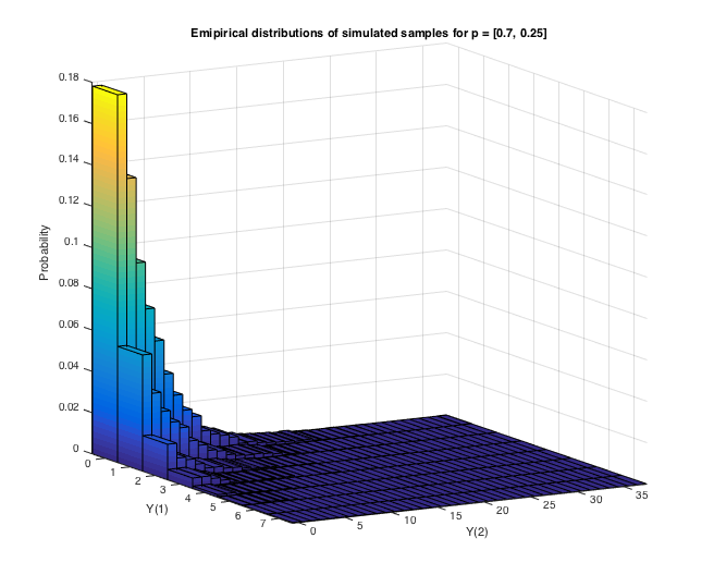
(a)

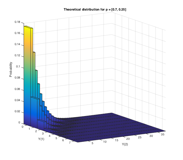
(b)

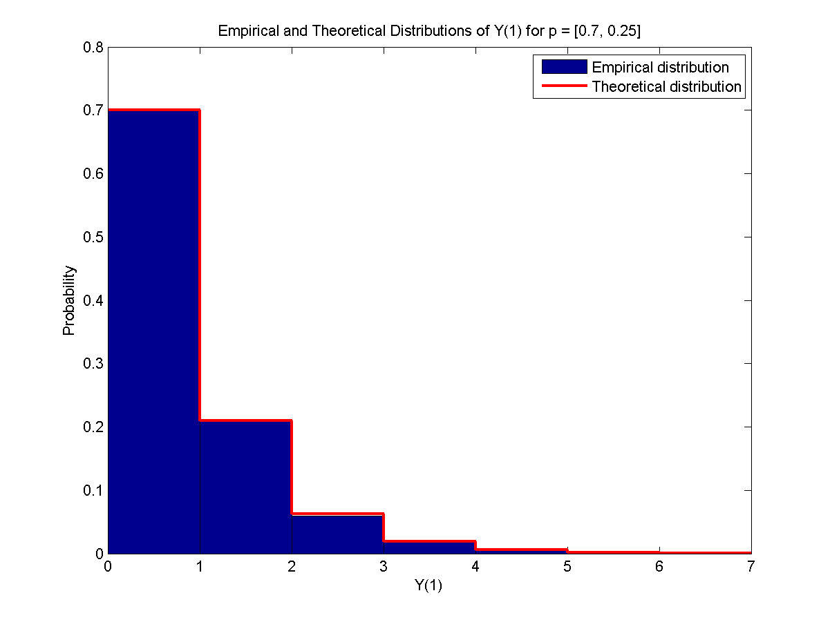
(c)

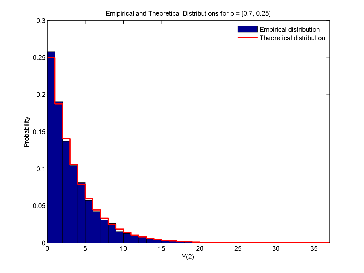
(d)

Figure 1. $\lambda=(0.225,0.717)$, $\mu=(1,1)$. (A) Histogram of the 10000 simulated samples of $(Y_{1}(\infty),Y_{2}(\infty))$. (B) Theoretic steady-state distribution of $(Y_{1}(\infty),Y_{2}(\infty))$. (C) Marginal distribution of $Y_{1}(\infty)$. (D) Marginal distribution of $Y_{2}(\infty)$.

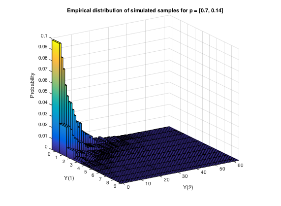
(a)

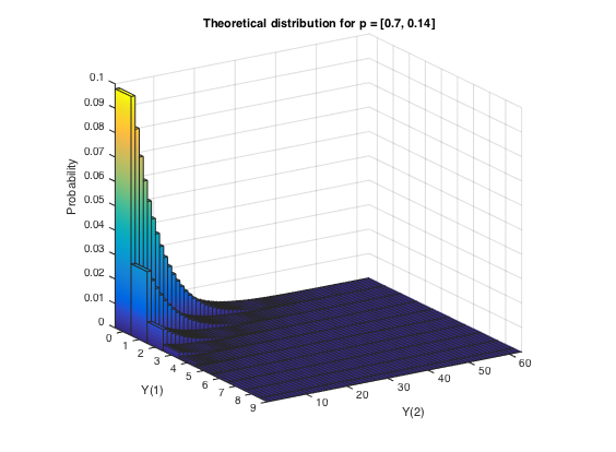
(b)

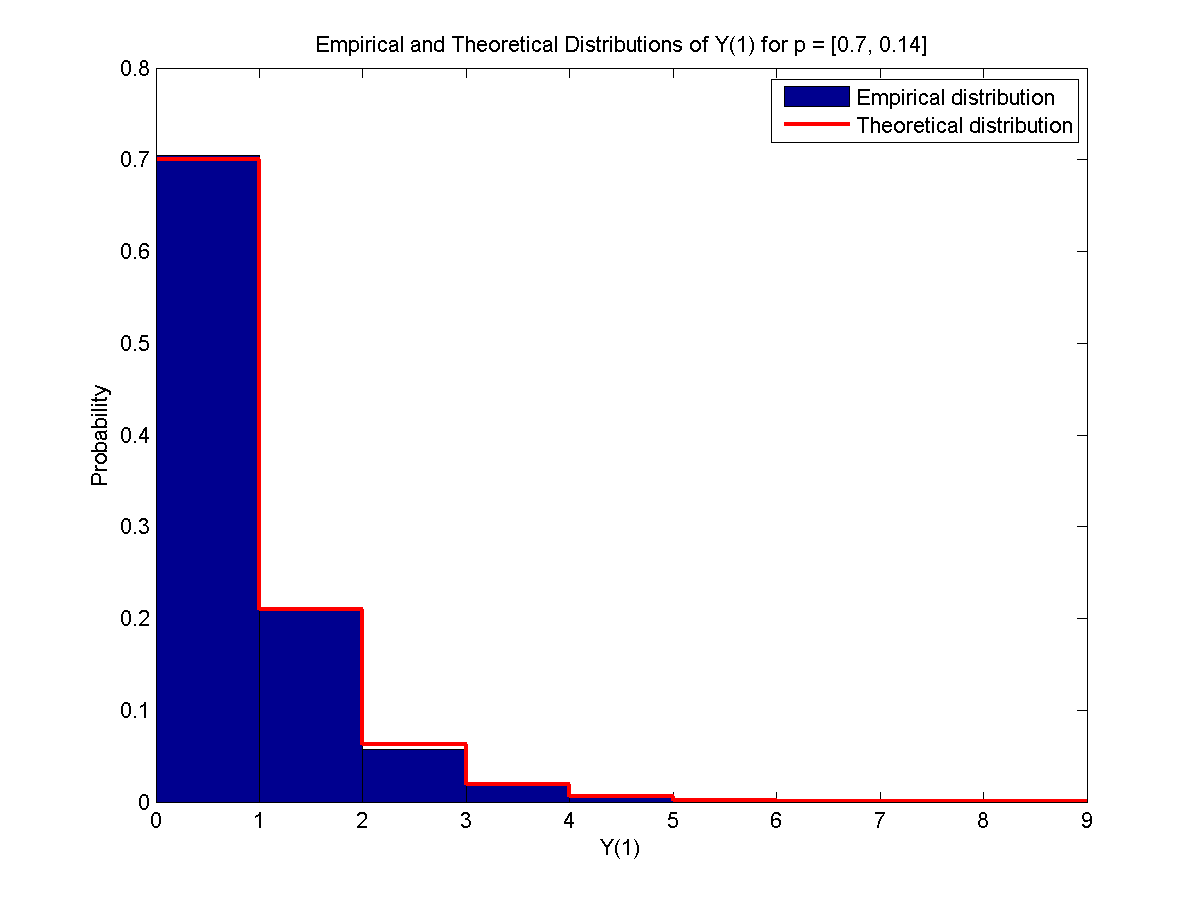
(c)

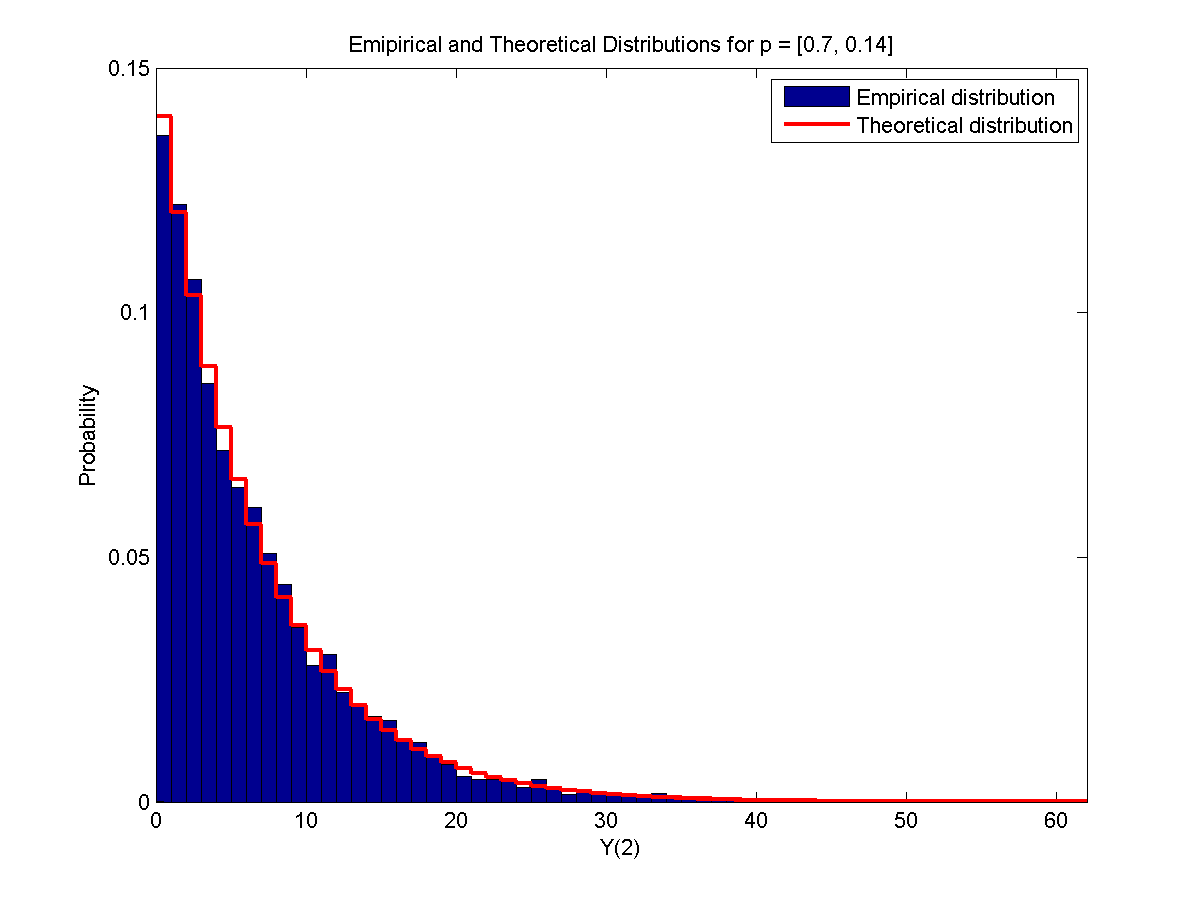
(d)

Figure 2. $\lambda=(0.214,0.827)$, $\mu=(1,1)$. (A) Histogram of the 10000 simulated samples of $(Y_{1}(\infty),Y_{2}(\infty))$. (B) Theoretic steady-state distribution of $(Y_{1}(\infty),Y_{2}(\infty))$. (C) Marginal distribution of $Y_{1}(\infty)$. (D) Marginal distribution of $Y_{2}(\infty)$.

7. Appendix: Technical Proofs

7.1. Technical Lemmas and the Proof of Theorem 1 .

Part i) of Theorem 1 is a restatement of Lemma 4.2 in [5]. Then, part ii) follows from the next lemma.

Lemma 4.

Suppose we start the coupled systems $\mathcal{N}^{+}$ and $\mathcal{N}^{\prime}$ empty from time $0$. Then for any $t>0$, when $Y_{i}^{\prime}(t)=y_{i}$, then the service station $i$ in system $\mathcal{N}^{+}$ must be one of the three following cases:

1. $Y^{+}_{i}(t)=y_{i}+1$ and the server is in service

2. $Y^{+}_{i}(t)=y\in\{1,2,...,y_{i}\}$ and the server is either in service or vacation

3. $Y_{i}^{+}(t)=0$ and the server is in vacation.

Proof of Lemma 4: The result follows directly by comparing the evolution of $Y_{i}^{\prime}(\cdot)$ given by (5), against the evolution of the number of customers waiting in the $i$-th queue of $\mathcal{N}^{+}$, namely $\widehat{Y}_{i}^{+}\left(\cdot\right)$, which satisfies (3.4). The equations are monotone with respect to the input process, which is strictly smaller for the network $\mathcal{N}^{+}$ compared to $\mathcal{N}^{\prime}$ because

$$\sum_{j:j\neq i,1\leq j\leq d}I(\widehat{S}_{j}^{+}\left(t_{-}\right)>0)\text{d}D_{j,i}\left(t\right)\leq\sum_{j:j\neq i,1\leq j\leq d}\text{d}D_{j,i}\left(t\right).$$

So, we conclude that $\widehat{Y}_{i}^{+}\left(t\right)\leq Y_{i}^{\prime}(t)$. Therefore, if $Y_{i}^{\prime}(t)=y_{i}$, we have $\widehat{Y}_{i}^{+}\left(t\right)\leq y_{i}$. As $\widehat{Y}_{i}^{+}\left(t\right)$ is the number of customers who are waiting for entering service, we can conclude that either $Y_{i}^{+}(t)=\widehat{Y}_{i}^{+}\left(t\right)+1$ if the server is in service and $Y_{i}^{+}(t)=\widehat{Y}_{i}^{+}\left(t\right)$ if the server is on vacation, and hence we are done. $\Box$

In order to prove part iii) of Theorem 1 we introduce some notation.

Let $y=(y_{1},...,y_{d})$ be a fixed vector in $\mathbb{N}_{0}^{d}=\{0,1,...\}^{d}$. Consider three vacation networks $\mathcal{N}^{+}$, $\mathcal{N}^{++}$, $\mathcal{N}^{+-}$ that have the same network topology and are driven by the same arrival and activity sequences, namely, $(A_{i}\left(n\right):n\geq 0)$ and $(\upsilon_{i}^{0}\left(n\right),r_{i}\left(n\right):n\geq 1)$, except for their initial state at time $0$. In particular, we set $Y_{i}^{++}(0)=y_{i}+1$ with all servers in service for all $i$, and $Y_{i}^{+-}(0)=0$ with all servers in vacation. The state of each service station in $\mathcal{N}^{+}$ at time $0$ is of any one of three cases as described in Lemma 4. More precisely, we have the following system of SDEs for $\widehat{Y}_{i}^{++}$, $\widehat{S}_{i}^{++}$, and $Y_{i}^{++}$ with $i\in\{1,...,d\}$,

$$\text{d}\widehat{Y}_{i}^{++}\left(t\right) =\text{d}N_{0,i}\left(t\right)+\sum_{j:j\neq i,1\leq j\leq d}I(\widehat{S}_{j}^{++}\left(t_{-}\right)>0)\text{d}D_{j,i}\left(t\right)-I(\widehat{Y}_{i}^{++}\left(t_{-}\right)>0)\text{d}D_{i}\left(t\right),$$

$$\text{d}\widehat{S}_{i}^{++}\left(t\right) =(I(\widehat{Y}_{i}^{++}\left(t_{-}\right)>0)-I(\widehat{S}_{i}^{++}\left(t_{-}\right)>0))\text{d}D_{i}\left(t\right),$$

$$\widehat{Y}_{i}^{++}\left(0\right) =y_{i}+1,\text{ }\widehat{S}_{i}^{++}\left(0\right)=1,$$

$$Y_{i}^{++}\left(t\right) =\widehat{Y}_{i}^{++}\left(t\right)+\widehat{S}_{i}^{++}\left(t\right).$$

The SDEs for $\widehat{Y}_{i}^{+},\widehat{S}_{i}^{+}$, $Y_{i}^{+}$, and $\widehat{Y}_{i}^{+-},\widehat{S}_{i}^{+-}$, $Y_{i}^{+-}$are exactly the same, except for the boundary conditions. In particular, $\widehat{Y}_{i}^{+}\left(0\right)=y_{i},$ $\widehat{S}_{i}^{++}\left(0\right)\in\{0,1\}$, and $\widehat{Y}_{i}^{+-}\left(0\right)=0,$ $\widehat{S}_{i}^{+-}\left(0\right)=0$. Then we have the following comparison result which implies part iii) of Theorem 1:

Lemma 5.

In order to distinguish servers whenever there might be ambiguity we shall call the server of the $i$-th service station in $\mathcal{N}^{++}$ the server $i^{+}$, the server of the $i$-th station in $\mathcal{N}^{+}$ is called server $i$, and the $i$-th server in $\mathcal{N}^{+-}$ is called $i^{-}$. We claim that the following three statements hold for all servers $i$, $i^{+}$, and $i^{-}$ $(i=1,2,...,d)$ and at any $t\geq 0$ (analogous statements to 2. and 3. hold replacing $i^{+}$ by $i$ and $i$ by $i^{-}$)

1. $Y_{i}^{++}(t)\geq Y_{i}^{+}(t)\geq Y_{i}^{+-}(t)$.

2. If $Y_{i}^{++}(t)=Y_{i}^{+}(t)$, server $i^{+}$ and server $i$ are both in service or both in vacation. Similarly, $Y_{i}^{+}(t)=Y_{i}^{+-}(t)$, server $i$ and server $i^{-}$ are both in service or both in vacation

3. If server $i^{+}$ is in vacation, server $i$ is also in vacation. Similarly, if $i$ is in vacation, server $i^{-}$ is also in vacation.

Proof of Lemma 5: Let’s first prove $Y_{i}^{++}(t)\geq Y_{i}^{+}(t)$.

First let’s check if the claim is true for $t=0$. Note that $Y_{i}^{++}(0)=y_{i}+1$ and $Y_{i}^{+}\in\{0,1,...,y_{i}+1\}$ and hence Statement (1) holds. As server $i^{+}$ is in service at time 0, Statement (2) also hold. Finally, if $Y_{i}^{+}(0)=Y_{i}^{++}(0)=y_{i}+1$, service station $i$ is of the first case in Lemma 4 which means both server $i$ and $i^{+}$ are at service. In summary, the claim is true for $t=0$.

Let $E(t)=\sum_{i=1}^{d}N_{0,i}(t)+\sum_{i=1}^{d}D_{i}(t)$ be the counting process of events that occur in the network. Define $t(n)=\inf\{t\geq 0:E(t)=n\}$ to be the time at which the $n$-th event occurs for $n\geq 1$ and set $t\left(0\right)=0$. We shall prove the statements 1-3 only for $i$ and $i^{+}$ first by induction on $n\geq 0$ at times $t\left(n\right)$, since there are no changes inside the network population between two event epochs. We have verified that statements 1-3 are valid at $t\left(0\right)$. Assume by induction hypothesis, that statements 1-3 hold for $t(n-1)$, we need to consider several cases at time $t(n)$.

Case 1: $t(n)$ corresponds to an arrival from $N_{0,i}(\cdot)$.
In this case, $Y_{i}^{++}(t(n))=Y_{i}^{++}(t(n-1))+1$ and $Y_{i}^{+}(t(n))=Y_{i}^{+}(t(n-1))+1$. According to the dynamics of vacation system, a new arrival from $N_{0,i}(\cdot)$ does not change the type of activity that is going on in servers $i^{+}$ and $i$. So statements 1-3 hold for server $i$ and $i^{+}$ at $t(n)$. As to all the other servers, there are no changes between $t(n-1)$ and $t(n)$. In summary, Statement 1-3 hold for all servers at $t(n)$.

Case 2: $t(n)$ corresponds to an arrival from $D_{i}(\cdot)$ and $Y_{i}^{++}(t(n-1))=Y_{i}^{+}(t(n-1))$.
By induction hypothesis, server $i$ and $i^{+}$ are in the same type of activity at time $t\left(n-1\right)$. Suppose that both servers $i$ and $i^{+}$ are at vacation at $t(n-1)$, it is clear from the dynamics that $Y_{i}^{++}(t(n))=Y_{i}^{+}(t(n))$. If $Y_{i}^{++}(t(n))>0$, it means that there was someone waiting and therefore at time $t\left(n\right)$, coming from vacation, now both $i^{+}$ and $i$ are now in service at time $t(n)$; otherwise, from the same logic, $Y_{i}^{++}(t(n))=0$, implies that both $i^{+}$ and $i$ are on vacation at $t(n)$. Besides, there are no changes on other servers between $t(n-1)$ and $t(n)$, because at $t(n-1)$ the servers where on vacation. Therefore, Statement 1-3 hold for all servers at $t(n)$.

If both server $i$ and $i^{+}$ are in service at $t(n-1)$ and $Y_{i}^{++}(t(n-1))=Y_{i}^{+}(t(n-1))=1$, then $Y_{i}^{++}(t(n))=Y_{i}^{+}(t(n))=0$ and both server $i^{+}$ and $i$ are in vacation at $t(n)$. Let $j=r_{i}(B_{i}(t(n)))$. If $j=0$, there are no changes on other servers between $t(n-1)$ and $t(n)$, so Statement 1-3 hold for all servers at $t(n)$. If $j>1$, then we can apply the argument of Case 1 to server $j$, $j^{+}$, and there are no changes on the rest servers other than $i^{+},i,$ $j^{+}$ and $j$. So statements 1-3 hold for all servers at $t=t(n)$.

If both server $i$ and $i^{+}$ are in service at $t(n-1)$ and $Y_{i}^{++}(t(n-1))=Y_{i}^{+}(t(n-1))>1$, the argument is similar to when $Y_{i}^{++}(t(n-1))=Y_{i}^{+}(t(n-1))=1$ except that now both server $i^{+}$ and $i$ are in service at $t(n)$.

Case 3: $t(n)$ corresponds to an arrival from $D_{i}(\cdot)$ and $Y_{i}^{++}(t(n-1))>Y_{i}^{+}(t(n-1))$

If server $i^{+}$ is in vacation at $t(n-1)$, by induction hypothesis, server $i$ is also in vacation at $t(n-1)$. Then, there are no changes on all other servers. Besides, $Y_{i}^{++}(t(n))=Y_{i}^{++}(t(n-1))$ and $Y_{i}^{+}(t(n))=Y_{i}^{+}(t(n-1))$ and hence $Y_{i}^{++}(t(n))>Y_{i}^{++}(t(n))$. As $Y_{i}^{++}(t(n))>0$, server $i^{+}$ is in service at $t(n)$ and hence we do not contradict statement 3 for servers $i^{+}$ and $i$ at time $t(n)$. In summary, we conclude that Statements 1-3 hold for all servers at time $t(n)$.

If server $i^{+}$ is in service and $Y_{i}^{++}(t(n-1))=1$ (and so $Y_{i}^{+}(t(n-1))=0$), $Y_{i}^{++}(t(n))=Y_{i}^{+}(t(n))=0$ and server $i^{+}$ and $i$ are both in vacation at time $t(n)$. Let $j=r_{i}(D_{i}(t(n)))$. If $j=0$, there are no changes on all other servers and hence statements 1-3 hold for all servers at $t(n)$. Otherwise, we have $Y_{j}^{++}(t(n))=Y_{j}^{++}(t(n-1))+1$ and $Y_{j}^{+}(t(n))=Y_{j}^{+}(t(n-1))$, as $Y_{j}^{++}(t(n-1))\geq Y_{j}^{+}(t(n-1))$ by induction hypothesis, $Y_{j}^{++}(t(n))>Y_{j}^{+}(t(n))$. So statement 1-2 hold for server $j^{+}$ and $j$. The type of activity that occurs in server $j^{+}$ and $j$ remains the same what was going on at time $t(n-1)$ and hence statement 3 holds. Since there are no changes on the rest servers other than $i^{+},i,j^{+}$ and $j$, statement 1-3 hold at time $t(n)$ for all servers.

If server $i^{+}$ is in service at $t(n-1)$ and $Y_{i}^{++}(t(n-1))>1$, $Y_{i}^{++}(t(n))=Y_{i}^{++}(t(n-1))-1>0$ and server $i^{+}$ is still in service at $t(n)$. So statement 3 holds for servers $i^{+}$ and $i$ at time $t(n)$. As $Y_{i}^{++}(t(n-1))\geq Y_{i}^{+}(t(n-1))+1$ and $Y_{i}^{+}(t(n))\geq Y_{i}^{+}(t(n))$, $Y_{i}^{++}(t(n))\geq Y_{i}^{+}(t(n))$ and statement 1 holds for server $i$. In case $Y_{i}^{++}(t(n))=Y_{i}^{+}(t(n))$, $Y_{i}^{+}(t(n))>0$ and hence both server $i^{+}$ and $i$ are in service at $t(n)$ and statement 2 holds. Following a similar argument as when server $i^{+}$ is in service at $t(n-1)$ and $Y_{i}^{+}(t(n-1))=1$, we can check that statement 1-3 hold for all the other servers. As a result, we can conclude that statement 1-2 hold at time $t(n)$ for all servers.

By induction, and by the nature of the processes, which changes only at times $t\left(n\right)$, statements 1-3 hold for all $t\geq 0$.

To prove that $Y_{i}^{+}(t)\geq Y_{i}^{+-}(t)$, we can use the same induction arguments simply replacing $Y_{i}^{++}(t)$ with $Y_{i}^{+}(t)$, and $Y_{i}^{+}(t)$ with $Y_{i}^{+-}(t)$ in statements 1-3. The induction part is exactly the same, so we are done if we can check that the three statements all hold at time $t\left(0\right)$.

As $Y_{i}^{+-}(0)=0$ and all servers $i^{-}$ are in vacation, statement 1-3 immediately hold. If $Y_{i}^{+}(0)=Y_{i}^{+-}(0)$, then $Y_{i}^{+}(0)=0$ and service station $i$ is in the last case as in Lemma 4, hence both $i$ and $i^{-}$ are in vacation and statement 2 holds. In summary, Statement 1-3 all hold for time $t\left(0\right)=0$ and thus the result follows. $\Box$

7.2. Recapitulation of the Main Procedure and Proof of Theorem 2

In order to prove Theorem 2, we need to recapitulate on the execution of our Main Procedure. Let us go back to equation (3.4) and allow us write

$$Y_{i}^{+}\left(t;T,y\right)=Y_{i}^{+}\left(t;T\right)$$

to recognize the boundary condition in (3.4). Moreover, we recall that $y_{i}=\bar{Y}_{i}^{\prime}\left(-T\right)$, from equation (7). For any $T>0$ define the event

$$C_{T}=\{\text{for all }t\in[0,T]\text{ there is }i\text{ such that }Y_{i}^{+}(k;T,\bar{Y}^{\prime}\left(-T\right))>0\}.$$

Then put $\bar{\tau}=\inf\{t\geq 0:\bar{C}_{t}$ occurs$\}$. Assuming that the output indeed follows the steady state distribution, the statement of Theorem 2 concerning the computational cost measure in terms of random numbers generated will follows if we can show that there exists $\delta>0$ such that $E[\exp\left(\delta\bar{\tau}\right)]<\infty$.

We start by noting that

$$P\left(\bar{\tau}>u\right)=P\left(C_{u}\right).$$

In order to compute $P\left(C_{n}\right)$ we can think forward in time, in particular consider

$$\text{d}\widehat{Y}_{i}^{+}\left(t;0,y\right) =\text{d}N_{0,i}\left(t;0\right)+\sum_{j:j\neq i,1\leq j\leq d}I(\widehat{S}_{j}^{+}\left(t_{-};0,y\right)>0)\text{d}D_{j,i}\left(t;0\right)-I(\widehat{Y}_{i}^{+}\left(t_{-};0,y\right)>0)\text{d}D_{i}\left(t;0\right),$$

$$\text{d}\widehat{S}_{i}^{+}\left(t;0,y\right) =(I(\widehat{Y}_{i}^{+}\left(t_{-};0,y\right)>0)-I(\widehat{S}_{i}^{+}\left(t_{-};0,y\right)>0))\text{d}D_{i}\left(t;0\right)\text{,}$$

$$\widehat{Y}_{i}^{+}\left(0;0,y\right) =y,\text{ }\widehat{S}_{i}^{+}\left(0;0,y\right)=1.$$

Note the relation between $D_{i}\left(t;0\right)$ and $D_{i}\left(-t\right)$, defined in (8), in particular $D_{i}(-t)=-D_{i}\left(t;0\right)\leq 0$ (similarly $N_{0,i}\left(-t\right)=N_{0,i}\left(t;0\right)$). Then let $Y_{i}^{+}\left(t;0,y\right)=\widehat{Y}_{i}^{+}\left(t;0,y\right)+\widehat{S}_{i}^{+}\left(t;0,y\right)$ we have that

$$P\left(C_{u}\right)=P\left(\text{for all }t\in[0,u]\text{, there is }i\text{ such that }Y_{i}^{+}\left(t;0,\bar{Y}^{\prime}\left(0\right)\right)>0\right).$$

The strategy is to first describe the evolution of $Y^{+}\left(\cdot;0,y\right)$ in terms of a Markov process. We need to track the residual times associated with each renewal process and the number of people both in queue and in service in each station. In particular, define

$$G_{i}\left(t\right)=\sup\{|A_{i}\left(-n\right)|:1\leq n\leq N_{0,i}\left(t;0\right)+1\}-t.$$

Similarly, we define

$$H_{i}\left(t\right)=\sup\{|B_{i}\left(-n\right)|:1\leq n\leq D_{i}\left(t;0\right)\}-t.$$

Then we let $t\left(n\right)$ be the times at which events occur, that is, $t\left(1\right)<t\left(2\right)<...$ are the discontinuity points of the process $\{E\left(t\right):t\geq 0\}$ defined as $E(t)=\sum_{i}N_{0,i}(t;0)+\sum_{i}D_{i}(t;0)$. Let us write $\Theta_{i}^{+}(n)=(\widehat{Y}_{i}^{+}(t(n)),\widehat{S}_{i}^{+}(t(n)))$ and define $\Xi^{+}\left(n\right)=(\Xi_{i}\left(n\right):1\leq i\leq d)$ as

$$\Xi_{i}^{+}\left(n\right)=(\Theta_{i}^{+}(n),G_{i}\left(t\left(n\right)\right),H_{i}\left(t\left(n\right)\right)).$$

Note that $\{\Xi^{+}\left(n\right):n\geq 0\}$ forms a Markov chain and we are given the initial condition $\Xi_{i}^{+}\left(0\right)=(\bar{Y}_{i}^{\prime}(0),1,G_{i}\left(0\right),H_{i}\left(0\right))$. Now, define

$$\tau\left(c\right)=\inf\{n\geq 0:\sum_{i=1}^{d}\Theta_{i}^{+}\left(n\right)\leq c\},$$

for some $c>0$. Following a similar approach to [7], due to Assumption 2, we now can show that there exists $c>0$ such that $E[\exp(\delta\tau\left(c\right))]<\infty$. Moreover, because the inter-arrivals have unbounded support a geometric trial argument will yield that if $\delta>0$ is chosen sufficiently small then $E[\exp\left(\delta\tau\left(0\right)\right)]<\infty$. In turn, this bound implies that $E[\exp\left(\delta\bar{\tau}\right)]<\infty$.

Next we want to show that the output indeed follows the target steady state distribution. This portion follows precisely from the validity of the DCFTP protocol.

Using the similar notation of $Y^{+}(t;T,y)$, we define $Y(t;T,y)$ as the number of customers in a GJN start with $Y(0;T,y)=y$ and is driven by the same sequence of inter-arrival times, service requirements and routing indices as $\mathcal{N}^{+}$ on $[-T,0]$. Given the comparison results in Theorem 1, given that $Y^{+}(-T^{\prime\prime})=0$, we can conclude that for all $T>T^{\prime\prime}$,

$$\sum_{i}Y_{i}(T-T^{\prime\prime};T,0)\leq\sum_{i}Y_{i}(T-T^{\prime\prime+}(-T))\leq\sum_{i}Y_{i}^{+}(T-T^{\prime\prime+}(-T))=\sum_{i}Y^{+}_{i}(-T^{\prime\prime})=0$$

and hence $Y(T-T^{\prime\prime};T,0)=0$. Therefore, for any $T>T^{\prime\prime}$

$$Y(T;T,0)=Y(T;T,Y(T-T^{\prime\prime};T,0))=Y(T^{\prime\prime};T^{\prime\prime},0).$$

As the process $Y(\cdot)$ has a unique stationary distribution (see [12]), we can conclude $Y(T^{\prime\prime};T^{\prime\prime},0)=\lim_{T\to\infty}Y(T;T,0)$ follows the stationary distribution.

Acknowledgement: Blanchet acknowledges support from the NSF through the grants CMMI-0846816 and 1069064. Chen acknowledges support from the NSF through the grant CMMI-1538102.

References

• [1] Blanchet, J. and Chen, X. (2014). Steady-state simulation of reflected Brownian motion and related stochastic networks. Annals of Applied Probability, Vol. 25, pp 3209-3250.
• [2] Blanchet, J. and Sigman, K. (2011). On exact sampling of stochastic perpetuities. Journal of Applied Probability, Special Vol. 48A, pp 165-183.
• [3] Blanchet, J. and Wallwater, A. (2014). Exact sampling of stationary and time-reversed queues. ACM Trans. Model. Comput. Sim., Vol. 25, Article 26.
• [4] Busic, A., Durand, S., Gaujal, B., Perronnin, F. (2015) Perfect sampling of Jackson queueing networks. Queueing Systems, Vol. 30, pp. 223-260.
• [5] Chang, C., Thomas, J. A. and Kiang, S. (1994). On the stability of open networks: a unified approach by stochastic dominance. Queueing Systems, Vol. 15, pp 239-260.
• [6] Ensor, K. B. and Glynn, P. W. (2000). Simulating the maximum of a random walk. Journal of Statistical Planning and Inference, Vol. 85, pp 127-135.
• [7] Gamarnik, D. and Zeevi, A. (2006). Validity of heavy traffic steady-state approximations in generalized Jackson networks. Annals of Applied Probability, Vol 16, pp 56-90.
• [8] Harrison, J. M. and Reiman, M. I. (1981). Reflected Brownian motion on an orthant. Annals of Probability, Vol. 9, pp 302-308
• [9] Kendall, W. (2004). Geometric ergodicity and perfect simulation. Electronic Communications in Probability, Vol. 9, pp 140-151.
• [10] Murdoch, D. J. and Takahara, G. (2006). Perfect sampling for queues and network models. TOMACS, Vol. 16, pp 76-92.
• [11] Propp, J. G. and Wilson, D. B. (1996). Exact sampling with coupled Markov chains and applications to statistical mechanics. Random Structures & Algorithms, Vol. 9, pp 223-252.
• [12] Sigman, K. (1990). The stability of open queueing networks. Stochastic Processes and their Applications, Vol. 35, pp 11-25.