Mathematical modeling and numerical simulation of a bioreactor landfill using Feel++

Abstract

In this paper, we propose a mathematical model to describe the functioning of a bioreactor landfill, that is a waste management facility in which biodegradable waste is used to generate methane. The simulation of a bioreactor landfill is a very complex multiphysics problem in which bacteria catalyze a chemical reaction that starting from organic carbon leads to the production of methane, carbon dioxide and water. The resulting model features a heat equation coupled with a non-linear reaction equation describing the chemical phenomena under analysis and several advection and advection-diffusion equations modeling multiphase flows inside a porous environment representing the biodegradable waste. A framework for the approximation of the model is implemented using Feel++, a C++ open-source library to solve Partial Differential Equations. Some heuristic considerations on the quantitative values of the parameters in the model are discussed and preliminary numerical simulations are presented.

Keywords: Bioreactor landfill; Multiphysics problem; Coupled problem; Finite Element Method; Feel++

1 Introduction

Waste management and energy generation are two key issues in nowadays societies. A major research field arising in recent years focuses on combining the two aforementioned topics by developing new techniques to handle waste and to use it to produce energy. A very active field of investigation focuses on bioreactor landfills which are facilities for the treatment of biodegradable waste. The waste is accumulated in a humid environment and its degradation is catalyzed by bacteria. The main process taking place in a bioreactor landfill is the methane generation starting from the consumption of organic carbon due to waste decomposition. Several by-products appear during this reaction, including carbon dioxide and leachate, that is a liquid suspension containing particles of the waste material through which water flows.

Several works in the literature have focused on the study of bioreactor landfills but to the best of our knowledge none of them tackles the global multiphysics problem. On the one hand, [21, 25, 20] present mathematical approaches to the problem but the authors deal with a single aspect of the phenomenon under analysis focusing either on microbiota activity and leachates recirculation or on gas dynamic. On the other hand, this topic has been of great interest in the engineering community [17, 3, 16] and several studies using both numerical and experimental approaches are available in the literature. We refer the interested reader to the review paper [1] on this subject.

In this work, we tackle the problem of providing a mathematical model for the full multiphysics problem of methane generation inside a bioreactor landfill. Main goal is the development of a reliable model to simulate the long-time behavior of these facilities in order to be able to perform forecasts and process optimization [19]. This paper represents a preliminary study of the problem starting from the physics of the phenomena under analysis and provides a first set of equations to describe the methane generation inside a bioreactor landfill. In a more general framework, we aim to develop a model sufficiently accurate to be applied to an industrial context limiting at the same time the required computational cost. Thus, a key aspect of this work focused on the identification of the most important features of the functioning of a bioreactor landfill in order to derive the simplest model possible to provide an accurate description of the aforementioned methanogenic phenomenon. The proposed model has been implemented using Feel++ and the resulting tool to numerically simulate the dynamic of a bioreactor landfill has been named SiViBiR++ which stands for Simulation of a Virtual BioReactor using Feel++.

The rest of the paper is organized as follows. After a brief description of the physical and chemical phenomena taking place inside these waste management facilities (Section 2), in section 3 we present the fully coupled mathematical model of a bioreactor landfill. Section 4 provides details on the numerical strategy used to discretize the discussed model. Eventually, in section 5 preliminary numerical tests are presented and section 6 summarizes the results and highlights some future perspectives. In appendix A, we provide a table with the known and unknown parameters featuring our model.

2 What is a bioreactor landfill?

As previously stated, a bioreactor landfill is a facility for the treatment of biodegradable waste which is used to generate methane, electricity and hot water. Immediately after being deposed inside a bioreactor, organic waste begins to experience degradation through chemical reactions. During the first phase, degradation takes place via aerobic metabolic pathways, that is a series of concatenated biochemical reactions which occur within a cell in presence of oxygen and may be accelerated by the action of some enzymes. Thus bacteria begin to grow and metabolize the biodegradable material and complex organic structures are converted to simpler soluble molecules by hydrolysis.

The aerobic degradation is usually short because of the high demand of oxygen which may not be fulfilled in bioreactor landfills. Moreover, as more material is added to the landfill, the layers of waste tend to be compacted and the upper strata begin to block the flow of oxygen towards the lower parts of the bioreactor. Within this context, the dominant reactions inside the facility become anaerobic. Once the oxygen is exhausted, the bacteria begin to break the previously generated molecules down to organic acids which are readily soluble in water and the chemical reactions involved in the metabolism provide energy for the growth of population of microbiota.

After the first year of life of the facility, the anaerobic conditions and the soluble organic acids create an environment where the methanogenic bacteria can proliferate [28]. These bacteria become the major actors inside the landfill by using the end products from the first stage of degradation to drive the methane fermentation and convert them into methane and carbon dioxide. Eventually, the chemical reactions responsible for the generation of these gases gradually decrease until the material inside the landfill is inert (approximately after 40 years).
In this work, we consider the second phase of the degradation process, that is the methane fermentation during the anaerobic stage starting after the first year of life of the bioreactor.

2.1 Structure of a bioreactor landfill

A bioreactor landfill counts several unit structures - named alveoli - as shown in the 3D rendering of a facility in Drouès, France (Fig. 1A). We focus on a single alveolus and we model it as a homogeneous porous medium in which the bulk material represents the solid waste whereas the void parts among the organic material are filled by a mixture of gases - mainly methane, carbon dioxide, oxygen, nitrogen and water vapor - and leachates, that is a liquid suspension based on water. For the rest of this paper, we will refer to our domain of interest by using indifferently the term alveolus and bioreactor, though the latter one is not rigorous from a modeling point of view.

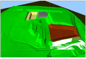
(A) 3D render of a bioreactor landfill.

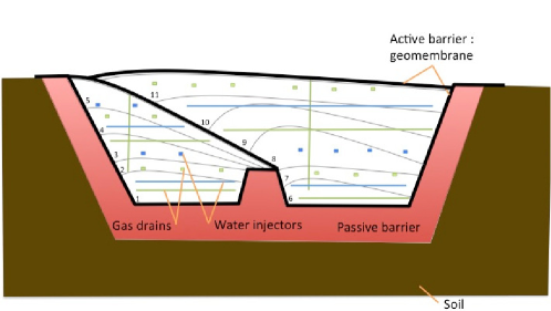
(B) Scheme of the structure of an alveolus.

Figure 1: Structure of a bioreactor landfill and its composing alveoli. Image courtesy of Entreprise Charier http://www.charier.fr.

Each alveolus is filled with several layers of biodegradable waste and the structure is equipped with a network of horizontal water injectors and production pipes respectively to allow the recirculation of leachates and to extract the gases generated by the chemical reactions. Moreover, each alveolus is isolated from the surrounding ground in order to prevent pollutant leaks and is covered by means of an active geomembrane. Figure 1B provides a schematic of an alveolus in which the horizontal pipes are organized in order to subdivide the structure in a cartesian-like way. Technical details on the construction and management of a bioreactor landfill are available in [14, 8].

2.2 Physical and chemical phenomena

Let us define the porosity $\phi$ as the fraction of void space inside the bulk material:

$$\phi=\frac{\textrm{Pore Volume}}{\textrm{Total Volume}}.$$ (2.1)

For biodegradable waste, we consider $\phi=0.3$ as by experimental measurements in [26], whereas it is known in the literature that for generic waste the value drops to $0.1$. Within this porous environment, the following phenomena take place:

• chemical reaction for the methane fermentation;

• heat transfer driven by the chemical reaction;

• transport phenomena of the gases;

• transport and diffusion phenomena of the leachates;

Here, we briefly provide some details about the chemical reaction for the methane generation, whereas we refer to section 3 for the description of the remaining phenomena and the derivation of the full mathematical model for the coupled system. As previously mentioned, at the beginning of the anaerobic stage the bacteria break the previously generated molecules down to organic acids, like the propionic acid $CH_{3}CH_{2}COOH$. This acid acts as a reacting term in the following reaction:

$$CH_{3}CH_{2}COOH+H_{2}O\longrightarrow 3\,H_{2}O+CO_{2}+2CH_{4}.$$ (2.2)

The microbiota activity drives the generation of methane ($CH_{4}$) and is responsible for the production of other by-products, mainly water ($H_{2}O$) and carbon dioxide ($CO_{2}$). As per equation (2.2), for each consumed mole of propionic acid - equivalently referred to as organic carbon with an abuse of notation -, two moles of methane are generated and three moles of water and one of carbon dioxide are produced as well.

Remark 2.1.

We remark that in order for reaction (2.2) to take place, water has to be added to the propionic acid. This means that the bacteria can properly catalyze the reaction only if certain conditions on the temperature and the humidity of the waste are fulfilled. This paper presents a first attempt to provide a mathematical model of a bioreactor landfill, thus both the temperature and the quantity of water inside the facility will act as unknowns in the model (cf. section 3). In a more general framework, the proposed model will be used to perform long-time forecasts of the methane generation process and the temperature and water quantity will have the key role of control variables of the system.

3 Mathematical model of a bioreactor landfill

In this section, we describe the equations modeling the phenomena taking place inside an alveolus. As stated in the introduction, the final goal of the SiViBiR++ project is to control and optimize the functioning of a real bioreactor landfill, hence a simple model to account for the phenomena under analysis is sought. Within this framework, in this article we propose a first mathematical model to describe the coupled physical and chemical phenomena involved in the methanogenic fermentation. In the following sections, we will provide a detailed description of the chemical reaction catalyzed by the methanogenic bacteria, the evolution of the temperature inside the alveolus and the transport phenomena driven by the dynamic of a mixture of gases and by the liquid water. An extremely important aspect of the proposed model is the interaction among the variables at play and consequently the coupling among the corresponding equations. In order to reduce the complexity of the model and to keep the corresponding implementation in Feel++ as simple as possible, some physical phenomena have been neglected. In the following subsections, we will detail the simplifying assumptions that allow to neglect some specific phenomena without degrading the reliability of the resulting model, by highlighting their limited impact on the global behavior of the overall system.

Let $\Omega\subset\mathbb{R}^{3}$ be an alveolus inside the landfill under analysis. We split the boundary $\partial\Omega$ of the computational domain into three non-void and non-overlapping regions $\Gamma_{\textrm{t}}$, $\Gamma_{\textrm{b}}$ and $\Gamma_{\textrm{l}}$, representing respectively the membrane covering the top surface of the bioreactor, the base of the alveolus and the ground surrounding the lateral surface of the structure.

3.1 Consumption of the organic carbon

As previously stated, the functioning of a bioreactor landfill relies on the consumption of biodegradable waste by means of bacteria. From the chemical reaction in (2.2), we may derive a relationship between the concentration of bacteria $b$ and the concentration of the consumable organic material which we denote by $C^{org}$.
The activity of the bacteria takes place if some environmental conditions are fulfilled, namely the waste humidity and the bioreactor temperature. Let $w_{\textrm{max}}$ and $T_{\textrm{opt}}$ be respectively the maximal quantity of water and the optimal temperature that allow the microbiota to catalyze the chemical reaction (2.2). We introduce the following functions to model the metabolism of the microbiota:

$$\Psi_{1}(w)=w\ \max\left(0,1-\frac{w}{w_{\textrm{max}}}\right),\qquad\Psi_{2}(T)=\max\left(0,1-\frac{|T-T_{\textrm{opt}}|}{A_{T}}\right)$$ (3.1)

where $A_{T}$ is the amplitude of the variation of the temperature tolerated by the bacteria. On the one hand, $\Psi_{1}$ models the fact that the bacterial activity is proportional to the quantity of liquid water - namely leachates - inside the bioreactor and it is prevented when the alveolus is flooded. On the other hand, according to $\Psi_{2}$ the microbiota metabolism is maximum when the current temperature equals $T_{\textrm{opt}}$ and it stops when it exceeds the interval of admissible temperatures $[T_{\textrm{opt}}-A_{T};T_{\textrm{opt}}+A_{T}]$.

Since the activity of the bacteria mainly consists in consuming the organic waste to perform reaction (2.2), it is straightforward to deduce a proportionality relationship between $b$ and $C^{\textrm{org}}$. By combining the information in (3.1) with this relationship, we may derive the following law to describe the evolution of the concentration of bacteria inside the bioreactor:

$$\partial_{t}b\propto b\ C^{\textrm{org}}\ \Psi_{1}(w)\ \Psi_{2}(T)$$ (3.2)

and consequently, we get a proportionality relationship for the consumption of the biodegradable material $C^{\textrm{org}}$:

$$\partial_{t}C^{\textrm{org}}\propto-\partial_{t}b.$$ (3.3)

Let $a_{b}$ and $c_{b}$ be two proportionality constants associated respectively with (3.2) and (3.3). By integrating (3.3) in time and introducing the proportionality constant $c_{b}$, we get that the concentration of bacteria reads as

$$b(x,t)=b_{0}+c_{b}(C^{\textrm{org}}_{0}-C^{\textrm{org}}(x,t))$$ (3.4)

where $b_{0}\coloneqq b(\cdot,0)$ and $C^{\textrm{org}}_{0}\coloneqq C^{\textrm{org}}(\cdot,0)$ are the initial concentrations respectively of bacteria and organic material inside the alveolus. Thus, by plugging (3.4) into (3.2) we get the following equation for the consumption of organic carbon between the instant $t=0$ and the final time $S^{\textrm{fin}}$:

$$\begin{cases}(1-\phi)\partial_{t}C^{\textrm{org}}(x,t)=-a_{b}\ b(x,t)\ C^{\textrm{org}}(x,t)\ \Psi_{1}(w(x,t))\ \Psi_{2}(T(x,t))\ ,\ &\text{in }\Omega\times(0,S^{\textrm{fin}}]\\ C^{\textrm{org}}(\cdot,0)=C^{\textrm{org}}_{0}\ ,\ &\text{in }\overline{\Omega}\end{cases}$$ (3.5)

We remark that the organic material filling the bioreactor is only present in the bulk part of the porous medium and this is modeled by the factor $1-\phi$ which features the information about the porosity of the environment. Moreover, we highlight that in equation (3.5) a non-linear reaction term appears and in section 4 we will discuss a strategy to deal with this non-linearity when moving to the Finite Element discretization.
For the sake of readability, from now on we will omit the dependency on the space and time variables in the notation for both the organic carbon and the concentration of bacteria.

3.2 Evolution of the temperature

The equation describing the evolution of the temperature $T$ inside the bioreactor is the classical heat equation with a source term proportional to the consumption of bacteria. We consider the external temperature to be fixed by imposing Dirichlet boundary conditions on $\partial\Omega$.

Remark 3.1.

Since we are interested in the long-time evolution of the system ($S^{\textrm{fin}}=40$ years), the unit time interval is sufficiently large to allow daily variations of the temperature to be neglected. Moreover, we assume that the external temperature remains constant during the whole life of the bioreactor. From a physical point of view, this assumption is not realistic but we conjecture that only small fluctuations would arise by the relaxation of this hypothesis. A future improvement of the model may focus on the integration of dynamic boundary conditions in order to model seasonal changes of the external temperature.

The resulting equation for the temperature reads as follows:

$$\begin{cases}\partial_{t}T(x,t)-k_{T}\Delta T(x,t)=-c_{T}\partial_{t}C^{\textrm{org}}(x,t)\ ,\ &\text{in}\ \Omega\times(0,S^{\textrm{fin}}]\\ T(x,\cdot)=T_{\textrm{m}}\ ,\ &\text{on}\ \Gamma_{\textrm{t}}\times(0,S^{\textrm{fin}}]\\ T(x,\cdot)=T_{\textrm{g}}\ ,\ &\text{on}\ \Gamma_{\textrm{b}}\cup\Gamma_{\textrm{l}}\times(0,S^{\textrm{fin}}]\\ T(\cdot,0)=T_{0}\ ,\ &\text{in}\ \overline{\Omega}\end{cases}$$ (3.6)

where $k_{T}$ is the thermal conductivity of the biodegradable waste and $c_{T}$ is a scaling factor that accounts for the heat transfer due to the chemical reaction catalyzed by the bacteria. The values $T_{\textrm{m}},\ T_{\textrm{g}}\ \text{and}\ T_{0}$ respectively represent the external temperature on the membrane $\Gamma_{\textrm{t}}$, the external temperature of the ground $\Gamma_{\textrm{b}}\cup\Gamma_{\textrm{l}}$ and the initial temperature inside the bioreactor.
For the sake of readability, from now on we will omit the dependency on the space and time variables in the notation of the temperature.

3.3 Velocity field of the gas

In order to model the velocity field of the gas inside the bioreactor, we have to introduce some assumptions on the physics of the problem. First of all, we assume the gas to be incompressible. This hypothesis stands if a very slow evolution of the mixture of gases takes place and this is the case for a bioreactor landfill in which the methane fermentation gradually decreases along the 40 years lifetime of the facility. Additionally, the decompression generated by the extraction of the gases through the pipes is negligible due to the weak gradient of pressure applied to the production system. Furthermore, we assume low Reynolds and low Mach numbers for the problem under analysis: this reduces to having a laminar slow flow which, as previously stated, is indeed the dynamic taking place inside an alveolus. Eventually, we neglect the effect due to the gravity on the dynamic of the mixture of gases: owing to the small height of the alveolus (approximately $90\text{\,}\mathrm{m}$), the variation of the pressure in the vertical direction due to the gravity is limited and in our model we simplify the evolution of the gas by neglecting the hydrostatic component of the pressure.

Under the previous assumptions, the behavior of the gas mixture inside a bioreactor landfill may be described by a mass balance equation coupled with a Darcy’s law

$$\begin{cases}\nabla\cdot u=0\ ,\ &\text{in}\ \Omega\\ u=-\nabla p\ ,\ &\text{in}\ \Omega\end{cases}$$ (3.7)

where $p\coloneqq\frac{D}{\phi\mu_{\text{gas}}}P$, $D$ is the permeability of the porous medium, $\phi$ its porosity and $\mu_{\text{gas}}$ the gas viscosity whereas $P$ is the pressure inside the bioreactor. In (3.7), the incompressibility assumption has been expressed by stating that the gas flow is isochoric, that is the velocity is divergence-free. This equation is widely used in the literature to model porous media (cf. e.g. [10, 18]) and provides a coherent description of the phenomenon under analysis in the bioreactor landfill. As a matter of fact, it is reasonable to assume that the density of the gas mixture is nearly constant inside the domain, owing to the weak gradient of pressure applied to extract the gas via the production system and to the slow rate of methane generation via the fermentation process, that lasts approximately 40 years.

To fully describe the velocity field, the effect of the production system that extracts the gases from the bioreactor has to be accounted for. We model the production system as a set of $N_{g}$ cylinders $\Theta_{g}^{i}$’s thus the effect of the gas extraction on each pipe results in a condition on the outgoing flow. Let $J_{\textrm{out}}>0$ be the mass flow rate exiting from the alveolus through each production pipe. The system of equations (3.7) is coupled with the following conditions on the outgoing normal flow on each drain used to extract the gas:

$$\int_{(\partial\Theta_{g}^{i})^{\textrm{n}}}(C^{\textrm{dx}}+M+O+N+h)\,u\cdot n\,d\sigma=J_{\textrm{out}}\;\qquad\forall i=1,\ldots,N_{g}.$$ (3.8)

In (3.8), $n$ is the outward normal vector to the surface, $(\partial\Theta_{g}^{i})^{\textrm{n}}$ is the part of the boundary of the cylinder $\Theta_{g}^{i}$ which belongs to the lateral surface of the alveolus itself and the term $(C^{\textrm{dx}}+M+O+N+h)$ represents the total concentration of the gas mixture starring carbon dioxide, methane, oxygen, nitrogen and water vapor.
Since the cross sectional area of the pipes belonging to the production system is negligible with respect to the size of the overall alveolus, we model these drains as 1D lines embedded in the 3D domain. Owing to this, in the following subsection we present a procedure to integrate the information (3.8) into a source term named $F^{\textrm{out}}$ in order to simplify the problem that describes the dynamic of the velocity field inside a bioreactor landfill.

Remark 3.2.

According to conditions (3.8), the velocity $u$ depends on the concentrations of the gases inside the bioreactor, thus is a function of both space and time. Nevertheless, the velocity field at each time step is independent from the previous ones and is only influenced by the distribution of gases inside the alveolus. For this reason, we neglect the dependency on the time variable and we consider $u$ being only a function of space.

3.3.1 The source term $F^{\textrm{out}}$

As previously stated, each pipe $\Theta_{g}^{i}$ is modeled as a cylinder of radius $R$ and length $L$. Hence, the cross sectional area $(\partial\Theta_{g}^{i})^{\textrm{n}}$ and the lateral surface $(\partial\Theta_{g}^{i})^{\textrm{l}}$ respectively measure $\pi R^{2}$ and $2\pi RL$.
We assume the gas inside the cylinder to instantaneously exit the alveolus through its boundary $(\partial\Theta_{g}^{i})^{\textrm{n}}$, that is the outgoing flow (3.8) is equal to the flow entering the drain through its lateral surface. Thus we may neglect the gas dynamic inside the pipe and (3.8) may be rewritten as

$$\int_{(\partial\Theta_{g}^{i})^{\textrm{n}}}(C^{\textrm{dx}}+M+O+N+h)\,u\cdot n\,d\sigma=\int_{(\partial\Theta_{g}^{i})^{\textrm{l}}}(C^{\textrm{dx}}+M+O+N+h)\,u\cdot n\,d\sigma=J_{\textrm{out}}\qquad\forall i=1,\ldots,N_{g}.$$ (3.9)

Moreover, under the hypothesis that the quantity of gas flowing from the bioreactor to the inside of the cylinder $\Theta_{g}^{i}$ is uniform over its lateral surface, that is the same gas mixture surrounds the drain in all the points along its dominant size, we get

$$\left(\int_{(\partial\Theta_{g}^{i})^{\textrm{l}}}(C^{\textrm{dx}}+M+O+N+h)\,d\sigma\right)u\cdot n=J_{\textrm{out}}\,\;\text{on}\,\;(\partial\Theta_{g}^{i})^{\textrm{l}}\qquad\forall i=1,\ldots,N_{g}.$$ (3.10)

We remark that gas densities may be considered uniform along the perimeter of the cylinder only if the latter is small enough, that is the aforementioned assumption is likely to be true if the radius of the pipe is small in comparison with the size of the alveolus. Within this framework, (3.10) reduces to

$$u\cdot n=\frac{J_{\textrm{out}}}{\displaystyle 2\pi R\int_{\mathfrak{L}^{i}}(C^{\textrm{dx}}+M+O+N+h)\,dl}\,\;\text{on}\,\;(\partial\Theta_{g}^{i})^{\textrm{l}}\qquad\forall i=1,\ldots,N_{g}$$ (3.11)

where $\mathfrak{L}^{i}$ is the centerline associated with the cylinder $\Theta_{g}^{i}$. By coupling (3.7) with (3.11), we get the following PDE to model the velocity field:

$$\begin{cases}-\Delta p=0\ ,\ &\text{in}\ \Omega\\ \nabla p\cdot n=-\frac{\displaystyle J_{\textrm{out}}}{\displaystyle 2\pi R\int_{\mathfrak{L}^{i}}(C^{\textrm{dx}}+M+O+N+h)\,dl}\ ,\ &\text{on}\ (\partial\Theta_{g}^{i})^{\textrm{l}}\qquad\forall i=1,\ldots,N_{g}\end{cases}$$ (3.12)

Let us consider the variational formulation of problem (3.12): we seek $p\in H^{1}(\Omega)$ such that

$$\int_{\Omega}\nabla p\cdot\nabla\delta p\,dx=\sum_{i=1}^{N_{g}}-\frac{\displaystyle J_{\textrm{out}}}{\displaystyle 2\pi R\int_{\mathfrak{L}^{i}}(C^{\textrm{dx}}+M+O+N+h)\,dl}\,\int_{(\partial\Theta_{g}^{i})^{\textrm{l}}}\delta p\,d\sigma\qquad\forall\delta p\in\mathcal{C}^{1}_{0}(\Omega).$$ (3.13)

We may introduce the term $F^{\textrm{out}}$ as the limit when $R$ tends to zero of the right-hand side of (3.13):

$$F^{\textrm{out}}\coloneqq\sum_{i=1}^{N_{g}}-\frac{\displaystyle J_{\textrm{out}}}{\displaystyle\int_{\mathfrak{L}^{i}}(C^{\textrm{dx}}+M+O+N+h)\,dl}\delta_{\mathfrak{L}^{i}}$$ (3.14)

where $\delta_{\mathfrak{L}^{i}}$ is a Dirac mass concentrated along the centerline $\mathfrak{L}^{i}$ of the pipe $\Theta_{g}^{i}$.
Hence, the system of equations describing the evolution of the velocity inside the alveolus may be written as

$$\begin{cases}\nabla\cdot u=F^{\textrm{out}}\ ,\ &\text{in}\ \Omega\\ u=-\nabla p\ ,\ &\text{in}\ \Omega\\ u\cdot n=0\ ,\ &\text{on}\ \partial\Omega\end{cases}$$ (3.15)

where the right-hand side of the mass balance equation may be either (3.14) or a mollification of it.

3.4 Transport phenomena for the gas components

Inside a bioreactor landfill the pressure field is comparable to the external atmospheric pressure. This low-pressure does not provide the physical conditions for gases to liquefy. Hence, the gases are not present in liquid phase and solely the dynamic of the gas phases has to be accounted for. Within this framework, in section 3.5 we consider the case of water for which phase transitions driven by heat transfer phenomena are possible, whereas in the current section we focus on the remaining gases (i.e. oxygen, nitrogen, methane and carbon dioxide) which solely exist in gas phase.

Let $u$ be the velocity of the gas mixture inside the alveolus. We consider a generic gas whose concentration inside the bioreactor is named $G$. The evolution of $G$ fulfills the classical pure advection equation:

$$\begin{cases}\phi\partial_{t}G(x,t)+u\cdot\nabla G(x,t)=F^{G}(x,t)\ ,\ &\text{in}\ \Omega\times(0,S^{\textrm{fin}}]\\ G(\cdot,0)=G_{0}\ ,\ &\text{in}\ \overline{\Omega}\end{cases}$$ (3.16)

where $\phi$ is again the porosity of the waste. The source term $F^{G}(x,t)$ depends on the gas and will be detailed in the following subsections.

3.4.1 The case of oxygen and nitrogen

We recall that the oxygen concentration is named $O$, whereas the nitrogen one is $N$. Neither of these components appears in reaction (2.2) thus the associated source terms are $F^{O}(x,t)=F^{N}(x,t)=0$. The resulting equations (3.17) are closed by the initial conditions $O(\cdot,0)=O_{0}$ and $N(\cdot,0)=N_{0}$.

$$\begin{split}&\phi\partial_{t}O+u\cdot\nabla O=0\\ &\phi\partial_{t}N+u\cdot\nabla N=0\\ \end{split}$$ (3.17)

Both the oxygen and the nitrogen are extracted by the production system thus their overall concentration may be negligible with respect to the quantity of carbon dioxide and methane inside the alveolus. Hence, for the rest of this paper we will neglect equations (3.17) by considering $O(x,t)\simeq O_{0}\simeq 0$ and $N(x,t)\simeq N_{0}\simeq 0$.

3.4.2 The case of methane and carbon dioxide

As previously stated, (2.2) describes the methanogenic fermentation that starting from the propionic acid drives the production of methane, having carbon dioxide as by-product. Equation (3.16) stands for both the methane $M$ and the carbon dioxide $C^{\textrm{dx}}$. For these components, the source terms have to account for the production of gas starting from the transformation of biodegradable waste. Thus, the source terms are proportional to the consumption of the quantity $C^{\textrm{org}}$ through some constants $c_{M}$ and $c_{C}$ specific to the chemical reaction and the component:

$$F^{j}(x,t)=-c_{j}\partial_{t}C^{\textrm{org}}\quad,\quad j=M,C$$

In a similar fashion as before, the resulting equations read as

$$\begin{split}&\phi\partial_{t}M+u\cdot\nabla M=-c_{M}\partial_{t}C^{\textrm{org}}\\ &\phi\partial_{t}C^{\textrm{dx}}+u\cdot\nabla C^{\textrm{dx}}=-c_{C}\partial_{t}C^{\textrm{org}}\\ \end{split}$$ (3.18)

and they are coupled with appropriate initial conditions $M(\cdot,0)=M_{0}$ and $C^{\textrm{dx}}(\cdot,0)=C^{\textrm{dx}}_{0}$.

3.5 Dynamic of water vapor and liquid water

Inside a bioreactor landfill, water exists both in vapor and liquid phase. Let $h$ be the concentration of water vapor and $w$ the one of liquid water. The variation of temperature responsible for phase transitions inside the alveolus is limited, whence we do not consider a two-phase flow for the water but we describe separately the dynamics of the gas and liquid phases of the fluid. On the one hand, the water vapor inside the bioreactor landfill evolves as the gases presented in section 3.4: it is produced by the chemical reaction (2.2), it is transported by the velocity field $u$ and is extracted via the pipes of the production system; as previously stated, no effect of the gravity is accounted for. This results in a pure advection equation for $h$. On the other hand, the dynamic of the liquid water may be schematized as follows: it flows in through the injector system at different levels of the alveolus, is transported by a vertical field $u_{w}$ due to the effect of gravity and is spread within the porous medium. The resulting governing equation for $w$ is an advection-diffusion equation. Eventually, the phases $h$ and $w$ are coupled by a source term that accounts for phase transitions.

Owing to the different nature of the phenomena under analysis and to the limited rate of heat transfer inside a bioreactor landfill, in the rest of this section we will describe separately the equations associated with the dynamics of the water vapor and the liquid water, highlighting their coupling due to the phase transition phenomena.

3.5.1 Phase transitions

Two main phenomena are responsible for the production of water vapor inside a bioreactor landfill. On the one hand, vapor is a product of the chemical reaction (2.2) catalyzed by the microbiota during the methanogenic fermentation process. On the other hand, heat transfer causes part of the water vapor to condensate and part of the liquid water to evaporate.
Let us define the vapor pressure of water $P^{\textrm{vp}}$ inside the alveolus as the pressure at which water vapor is in thermodynamic equilibrium with its condensed state. Above this critical pressure, water vapor condenses, that is it turns to the liquid phase. This pressure is proportional to the temperature $T$ and may be approximated by the following Rankine law:

$$P^{\textrm{vp}}(T)=P_{0}\exp\left(s_{0}-\frac{s_{1}}{T}\right)$$ (3.19)

where $P_{0}$ is a reference pressure, $s_{0}$ and $s_{1}$ are two constants known by experimental results and $T$ is the temperature measured in Kelvin. If we restrict to a range of moderate temperatures, we can approximate the exponential in (3.19) by means of a linear law. Let $H_{0}$ and $H_{1}$ be two known constants, we get

$$P^{\textrm{vp}}(T)\simeq H_{0}+H_{1}T.$$ (3.20)

Let $P^{h}$ be the partial pressure of the water vapor inside the gas mixture. We can compute $P^{h}$ multiplying the total pressure $p$ by a scaling factor representing the ratio of water vapor inside the gas mixture:

$$P^{h}=\frac{h}{C^{\textrm{dx}}+M+O+N+h}p.$$ (3.21)

The phase transition process features two different phenomena. On the one hand, when the pressure $P^{h}$ is higher than the vapor pressure of water $P^{\textrm{vp}}$ the vapor condensates. By exploiting (3.21) and (3.20), the condition $P^{h}>P^{\textrm{vp}}(T)$ may be rewritten as

$$h-H(T)>0\qquad,\qquad H(T)\coloneqq(C^{\textrm{dx}}+M+O+N+h)\frac{H_{0}+H_{1}T}{p}.$$

We assume the phase transition to be instantaneous, thus the condensation of water vapor may be expressed through the following function

$$F^{\textrm{cond}}\coloneqq c_{h\to w}\max(h-H(T),0)$$ (3.22)

where $c_{h\to w}$ is a scaling factor. As per (3.22), the production of vapor from liquid water is $0$ as soon as the concentration of vapor is larger than the threshold $H(T)$, that is the air is saturated.
In a similar fashion, we may model the evaporation of liquid water. When $P^{h}$ is below the vapor pressure of water $P^{\textrm{vp}}$ - that is $h-H(T)<0$ - part of the liquid water generates vapor. The evaporation rate is proportional to the difference $P^{\textrm{vp}}(T)-P^{h}$ and to the quantity of liquid water $w$ available inside the alveolus. Hence, the evaporation of liquid water is modeled by the following expression

$$F^{\textrm{evap}}\coloneqq c_{w\to h}\max(H(T)-h,0)w.$$ (3.23)

Remark 3.3.

Since the quantity of water vapor inside a bioreactor landfill is negligible, we assume that the evaporation process does not significantly affect the dynamic of the overall system. Hence, in the rest of this paper, we will neglect this phenomenon by modeling only the condensation (3.22).

3.5.2 The case of water vapor

The dynamic of the water vapor may be modeled using (3.16) as for the other gases. In this case, the source term has to account for both the production of water vapor due to the chemical reaction (2.2) and its decrease as a consequence of the condensation phenomenon:

$$F^{h}(x,t)\coloneqq-c_{h}\partial_{t}C^{\textrm{org}}-F^{\textrm{cond}}$$

where $c_{h}$ is a scaling factor describing the relationship between the consumption of organic carbon and the generation of water vapor. The resulting advection equation reads as

$$\phi\partial_{t}h+u\cdot\nabla h=-c_{h}\partial_{t}C^{\textrm{org}}-F^{\textrm{cond}}$$ (3.24)

and it is coupled with the initial condition $h(\cdot,0)=h_{0}$.

3.5.3 The case of liquid water

The liquid water inside the bioreactor is modeled by an advection-diffusion equation in which the drift term is due to the gravity, that is the transport phenomenon is mainly directed in the vertical direction and is associated with the liquid flowing downward inside the alveolus.

$$\begin{cases}\phi\partial_{t}w(x,t)+u_{w}\cdot\nabla w(x,t)-k_{w}\Delta w(x,t)=F^{\textrm{cond}}(x,t)\ ,\ &\text{in}\ \Omega\times(0,S^{\textrm{fin}}]\\ k_{w}\nabla w(x,t)\cdot n=0\ \text{and}\ u_{w}\cdot n=0\ ,\ &\text{on}\ \Gamma_{\textrm{t}}\cup\Gamma_{\textrm{l}}\times(0,S^{\textrm{fin}}]\\ k_{w}\nabla w(x,t)\cdot n=0\ ,\ &\text{on}\ \Gamma_{\textrm{b}}\times(0,S^{\textrm{fin}}]\\ w(\cdot,0)=w_{0}\ ,\ &\text{in}\ \overline{\Omega}\end{cases}$$ (3.25)

where $u_{w}\coloneqq(0,0,-\|u_{w}\|)^{T}$ is the vertical velocity of the water and $k_{w}$ is its diffusion coefficient. The right-hand side of the first equation accounts for the water production by condensation as described in section 3.5.1. On the one hand, the free-slip boundary conditions on the lateral and top surfaces allow water to slide but prevent its exit, that is the top and lateral membranes are waterproof. On the other hand, the homogeneous Neumann boundary condition on the bottom of the domain describes the ability of the water to flow through this membrane. These conditions are consistent with the impermeability of the geomembranes and with the recirculation of leachates which are extracted when they accumulate in the bottom part of the alveolus and are reinjected in the upper layers of the waste management facility.

Remark 3.4.

It is well-known in the literature that the evolution of an incompressible fluid inside a given domain is described by the Navier-Stokes equation. In (3.25), we consider a simplified version of the aforementioned equation by linearizing the inertial term. As previously stated, the dynamic of the fluids inside the bioreactor landfill is extremely slow and we may assume a low Reynolds number regime for the water as well. Under this assumption, the transfer of kinetic energy in the turbulent cascade due to the non-linear term of the Navier-Stokes equation may be neglected. Moreover, by means of a linearization of the inertial term $(w\cdot\nabla)w$, the transport effect is preserved and the resulting parabolic advection-diffusion problem (3.25) may be interpreted as an unsteady version of the classical Oseen equation [9].

Remark 3.5.

Equation (3.25) may be furtherly interpreted as a special advection equation modeling the transport phenomenon within a porous medium. As a matter of fact, the diffusion term $-k_{w}\Delta w$ accounts for the inhomogeneity of the environment in which the water flows and describes the fact that the liquid spreads in different directions while flowing downwards due to the encounter of blocking solid material along its path. The distribution of the liquid into different directions is random and is mainly related to the nature of the surrounding environment thus we consider an isotropic diffusion tensor $k_{w}$. The aforementioned equation is widely used (cf. e.g. [27]) to model flows in porous media and is strongly connected with the description of the porous environment via the Darcy’s law introduced in section 3.3.
Within the framework of our problem, the diffusion term is extremely important since it models the spread of water and leachates inside the bioreactor landfill and the consequent humidification of the whole alveolus and not solely of the areas neighboring the injection pipes.

Eventually, problem (3.25) is closed by a set of conditions that describe the injection of liquid water and leachates through $N_{w}$ pipes $\Theta_{w}^{i}$’s. As previously done for the production system, we model each injector as a cylinder of radius $R$ and length $L$ and we denote by $(\partial\Theta_{w}^{i})^{\textrm{n}}$ and $(\partial\Theta_{w}^{i})^{\textrm{l}}$ respectively the part of the boundary of the cylinder which belongs to the boundary of the bioreactor and its lateral surface. The aforementioned inlet condition reads as

$$\int_{(\partial\Theta_{w}^{i})^{\textrm{n}}}k_{w}\nabla w\cdot n\,d\sigma=-J_{\textrm{in}}\;\qquad\forall i=1,\ldots,N_{w}$$

where $J_{\textrm{in}}>0$ is the mass flow rate entering the alveolus through each injector. As for the production system in section 3.3.1, we may now integrate this condition into a source term for equation (3.25). Under the assumption that the flow is instantaneously distributed along the whole cylinder in a uniform way, we get

$$\int_{(\partial\Theta_{w}^{i})^{\textrm{n}}}k_{w}\nabla w\cdot n\,d\sigma=-\int_{(\partial\Theta_{w}^{i})^{\textrm{l}}}k_{w}\nabla w\cdot n\,d\sigma=-J_{\textrm{in}}\qquad\forall i=1,\ldots,N_{w}.$$

Consequently the condition on each injector reads as

$$k_{w}\nabla w\cdot n=\frac{J_{\textrm{in}}}{2\pi RL}\,\;\text{on}\,\;(\partial\Theta_{w}^{i})^{\textrm{l}}\qquad\forall i=1,\ldots,N_{w}$$

and we obtain the following source term $F^{\textrm{in}}$

$$F^{\textrm{in}}\coloneqq\sum_{i=1}^{N_{w}}\frac{\displaystyle J_{\textrm{in}}}{\displaystyle L}\delta_{\mathfrak{L}^{i}}$$ (3.26)

where $\delta_{\mathfrak{L}^{i}}$ is a Dirac mass concentrated along the centerline $\mathfrak{L}^{i}$ of the pipe $\Theta_{w}^{i}$. Hence, the resulting dynamic of the liquid water inside an alveolus is modeled by the following PDE:

$$\begin{cases}\phi\partial_{t}w+u_{w}\cdot\nabla w-k_{w}\Delta w=F^{w}\ ,\ &\text{in}\ \Omega\times(0,S^{\textrm{fin}}]\\ k_{w}\nabla w\cdot n=0\ \text{and}\ u_{w}\cdot n=0\ ,\ &\text{on}\ \Gamma_{\textrm{t}}\cup\Gamma_{\textrm{l}}\times(0,S^{\textrm{fin}}]\\ k_{w}\nabla w\cdot n=0\ ,\ &\text{on}\ \Gamma_{\textrm{b}}\times(0,S^{\textrm{fin}}]\\ \end{cases}$$ (3.27)

with $F^{w}\coloneqq F^{\textrm{cond}}+F^{\textrm{in}}$ and the initial condition $w(\cdot,0)=w_{0}$. By analyzing the right-hand side of equation (3.27), we remark that neglecting the effect of evaporation in the phase transition allows to decouple the dynamics of liquid water and water vapor. Moreover, as previously stated for equation (3.15), $F^{\textrm{in}}$ may be chosen either according to definition (3.26) or by means of an appropriate mollification.

4 Numerical approximation of the coupled system

This section is devoted to the description of the numerical strategies used to discretize the fully coupled model of the bioreactor landfill introduced in section 3. We highlight that one of the main difficulties of the presented model is the coupling of all the equations and the multiphysics nature of the problem under analysis. Here we propose a first attempt to discretize the full model by introducing an explicit coupling of the equations, that is by considering the source term in each equation as function of the variables at the previous iteration.

4.1 Geometrical model of an alveolus

As previously stated, a bioreactor landfill is composed by several alveoli. Each alveolus may be modeled as an independent structure obtained starting from a cubic reference domain (Fig. 2A) to which pure shear transformations are applied (Fig. 2B-2C).

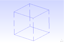
(A) Cubic reference domain.

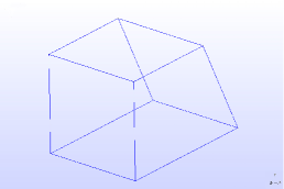
(B) Lateral shear on a face.

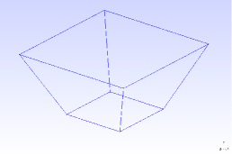
(C) Pyramidal domain.

Figure 2: Reference domain for an alveolus and admissible transformations.

For example, the pure lateral shear in figure 2B allows to model the left-hand side alveolus in figure 1B whereas the right-hand side one may be geometrically approximated by means of the pyramid in figure 2C.
In order to model the network of the water injectors and the one of the drains extracting the gas, the geometrical domains in figure 2 are equipped with a cartesian distribution of horizontal lines, the 1D model being justified by the assumption in section 3.

4.2 Finite Element approximations of the organic carbon and heat equations

Both equations (3.5) and (3.6) are discretized using Lagrangian Finite Element functions. In particular, the time derivative is approximated by means of an implicit Euler scheme, whereas the basis functions for the spatial discretization are the classical $\mathbb{P}_{k}$ Finite Element functions of degree $k$.
Let $t=t_{n}$. We consider the following quantities at time $t_{n}$ as known variables: $C^{\textrm{org}}_{n}\coloneqq C^{\textrm{org}}(x,t_{n})$, $T_{n}\coloneqq T(x,t_{n})$ and $w_{n}\coloneqq w(x,t_{n})$. The consumption of organic carbon is described by equation (3.5) coupled with equation (3.4) for the dynamic of the bacteria. At each time step, we seek $C^{\textrm{org}}_{n+1}\in H^{1}(\Omega)$ such that

$$\int_{\Omega}(1-\phi)\frac{C^{\textrm{org}}_{n+1}-C^{\textrm{org}}_{n}}{\Delta t}\delta C\,dx=-\int_{\Omega}a_{b}\ C^{\textrm{org}}_{n+1}\left[b_{0}+c_{b}(C^{\textrm{org}}_{0}-C^{\textrm{org}}_{n})\right]\Psi_{1}(w_{n})\ \Psi_{2}(T_{n})\ \delta C\,dx\qquad\forall\delta C\in H^{1}(\Omega)$$

We remark that in the previous equation the non-linear reaction term has been handled in a semi-implicit way by substituting $(C^{\textrm{org}}_{n+1})^{2}$ by $C^{\textrm{org}}_{n+1}C^{\textrm{org}}_{n}$ in the right-hand side. Hence, the bilinear and linear forms associated with the variational formulation at $t=t_{n}$ respectively read as

$$a_{C^{\textrm{org}}}(C^{\textrm{org}}_{n+1},\delta C)=\int_{\Omega}A_{C}\ C^{\textrm{org}}_{n+1}\ \delta C\,dx\qquad,\qquad l_{C^{\textrm{org}}}(\delta C)=\int_{\Omega}(1-\phi)\ C^{\textrm{org}}_{n}\ \delta C\,dx$$ (4.1)

where $A_{C}=(1-\phi)+\Delta t\ a_{b}\left[b_{0}+c_{b}(C^{\textrm{org}}_{0}-C^{\textrm{org}}_{n})\right]\Psi_{1}(w_{n})\ \Psi_{2}(T_{n})$ and $a_{C^{\textrm{org}}}(C^{\textrm{org}}_{n+1},\delta C)=l_{C^{\textrm{org}}}(\delta C)\ \forall\delta C\in H^{1}(\Omega)$.

In a similar fashion, we derive the variational formulation of the heat equation and at $t=t_{n}$ we seek $T_{n+1}\in H^{1}(\Omega)$ such that $T_{n+1}|_{\Gamma_{\textrm{t}}}=T_{\textrm{m}}$, $T_{n+1}|_{\Gamma_{\textrm{b}}\cup\Gamma_{\textrm{l}}}=T_{\textrm{g}}$ and $a_{T}(T_{n+1},\delta T)=l_{T}(\delta T)\ \forall\delta T\in H^{1}_{0}(\Omega)$, where

$$a_{T}(T_{n+1},\delta T)=\int_{\Omega}\ T_{n+1}\ \delta T\,dx+\Delta t\int_{\Omega}\ k_{T}\nabla T_{n+1}\cdot\nabla\delta T\,dx\,,$$ (4.2)

$$l_{T}(\delta T)=\int_{\Omega}\ T_{n}\ \delta T\,dx-\int_{\Omega}c_{T}(C^{\textrm{org}}_{n+1}-C^{\textrm{org}}_{n})\ \delta T\,dx.$$ (4.3)

Remark 4.1.

In (4.2) and (4.3), we evaluate the time derivative $\partial_{t}C^{\textrm{org}}$ at $t=t_{n}$, that is we consider the current value and not the previous one as stated at the beginning of this section. This is feasible because the solution of problem (4.1) precedes the one of the heat equation thus the value $C^{\textrm{org}}_{n+1}$ is known when solving (4.2)-(4.3).

Remark 4.2.

In (4.3) we assume that the same time discretization is used for both the organic carbon and the temperature. If this is not the case, the second term in the linear form $l_{T}(\cdot)$ would feature a scaling factor $\frac{\Delta t_{T}}{\Delta t_{C}}$, the numerator being the time scale associated with the temperature and the denominator the one for the organic carbon. For the rest of this paper, we will assume that all the unknowns are approximated using the same time discretization.

By substituting $C^{\textrm{org}}_{n}$ and $T_{n}$ with their Finite Element counterparts $C^{\textrm{org}}_{h,n}$ and $T_{h,n}$ in (4.1), (4.2) and (4.3) we obtain the corresponding discretized equations for the organic carbon and the temperature.

4.3 Stabilized dual-mixed formulation of the velocity field

A good approximation of the velocity field is a key point for a satisfactory simulation of all the transport phenomena. In order for problem (3.15) to be well-posed, the following compatibility condition has to be fulfilled

$$\int_{\Omega}F^{\textrm{out}}=0.$$ (4.4)

Nevertheless, (4.4) does not stand for the problem under analysis thus we consider a slightly modified version of problem (3.15) by introducing a small perturbation parameter $\lambda=\mathcal{O}(\ell_{K})$, $\ell_{K}$ being the diameter of the element $K$ of the triangulation $\mathcal{T}_{h}$:

$$\begin{cases}\nabla\cdot u+\lambda p=F^{\textrm{out}}\ ,\ &\text{in}\ \Omega\\ u=-\nabla p\ ,\ &\text{in}\ \Omega\\ u\cdot n=0\ ,\ &\text{on}\ \partial\Omega\\ \end{cases}$$ (4.5)

Hence the resulting problem (4.5) is well-posed even if (4.4) does not stand.

It is well-known in the literature [12] that classical discretizations of problem (4.5) by means of Lagrangian Finite Element functions lead to poor approximations of the velocity field. A widely accepted workaround relies on the derivation of mixed formulations in which a simultaneous approximation of pressure and velocity fields is performed by using different Finite Element spaces [24].

4.3.1 Dual-mixed formulation

Let $H(\operatorname{div})=\{v\in[L^{2}(\Omega)]^{3}\ \text{s.t.}\ \nabla\cdot v\in L^{2}(\Omega)\}$ and $H_{0}(\operatorname{div})=\{v\in H(\operatorname{div})\ \text{s.t.}\ v\cdot n=0\ \text{on}\ \partial\Omega\}$. The dual-mixed formulation of problem (4.5) is obtained by seeking $(u,p)\in H_{0}(\operatorname{div})\times L^{2}(\Omega)$ such that

$$\left\{\begin{aligned} &\int_{\Omega}{\nabla\cdot u\delta p\ dx}+\int_{\Omega}{\lambda p\delta p\ dx}=\int_{\Omega}{F^{\textrm{out}}\delta p\ dx}\\ &\int_{\Omega}{u\cdot\delta u\ dx}-\int_{\Omega}{p\nabla\cdot\delta u\ dx}=0\end{aligned}\right.\quad,\quad\forall(\delta u,\delta p)\in H_{0}(\operatorname{div})\times L^{2}(\Omega).$$

Hence, the bilinear and linear forms associated with the variational formulation of the problem respectively read as

$$a_{\textrm{vel}}(\{u,p\},\{\delta u,\delta p\})=\int_{\Omega}{u\cdot\delta u\ dx}-\int_{\Omega}{p\nabla\cdot\delta u\ dx}-\int_{\Omega}{\nabla\cdot u\delta p\ dx}-\int_{\Omega}{\lambda p\delta p\ dx}$$ (4.6)

$$l_{\textrm{vel}}(\{\delta u,\delta p\})=-\int_{\Omega}{F^{\textrm{out}}\delta p\ dx}$$ (4.7)

To overcome the constraint due to the LBB compatibility condition that the Finite Element spaces have to fulfill [5], several stabilization approaches have been proposed in the literature over the years and in this work we consider a strategy inspired by the Galerkin Least-Squares method and known as CGLS [11].

4.3.2 Galerkin Least-Squares stabilization

The GLS formulation relies on adding one or more quantities to the bilinear form of the problem under analysis in order for the resulting bilinear form to be strongly consistent and stable. Let $L$ be the abstract operator for the Boundary Value Problem $L\varphi=g$. We introduce the solution $\varphi_{h}$ of the corresponding problem discretized via the Finite Element Method. The GLS stabilization term reads as

$$\mathcal{L}^{\textrm{GLS}}(\varphi_{h},g;\psi_{h})=d\int_{\Omega}{(L\varphi_{h}-g)L\psi_{h}\ dx}.$$

GLS formulation of Darcy’s law

Following the aforementioned framework, we have

$$L_{1}(\{u,p\})=g_{1}\qquad\text{with}\qquad L_{1}(\{u,p\})\coloneqq u+\nabla p,\qquad g_{1}\coloneqq 0.$$

Thus the GLS term associated with Darcy’s law reads as

$$\mathcal{L}^{\textrm{GLS}}_{1}(\{u_{h},p_{h}\},g_{1};\{\delta u_{h},\delta p_{h}\})=d_{1}\int_{\Omega}{(u_{h}+\nabla p_{h})\cdot(\delta u_{h}+\nabla\delta p_{h})\ dx}.$$ (4.8)

GLS formulation of the mass balance equation

The equation describing the mass equilibrium may be rewritten as

$$L_{2}(\{u,p\})=g_{2}\qquad\text{with}\qquad L_{2}(\{u,p\})\coloneqq\nabla\cdot u+\lambda p,\qquad g_{2}\coloneqq F^{\textrm{out}}.$$

Consequently, the Least-Squares stabilization term has the following form

$$\mathcal{L}^{\textrm{GLS}}_{2}(\{u_{h},p_{h}\},g_{2};\{\delta u_{h},\delta p_{h}\})=\underbrace{d_{2}\int_{\Omega}{(\nabla\cdot u_{h}+\lambda p_{h})(\nabla\cdot\delta u_{h}+\lambda\delta p_{h})\ dx}}-\underbrace{d_{2}\int_{\Omega}{F^{\textrm{out}}(\nabla\cdot\delta u_{h}+\lambda\delta p_{h})\ dx}}.$$ (4.9)

$$\hskip 130.0pt\mathcal{L}^{\textrm{GLS}}_{2a}(\{u_{h},p_{h}\},g_{2};\{\delta u_{h},\delta p_{h}\})\hskip 30.0pt\mathcal{L}^{\textrm{GLS}}_{2l}(\{u_{h},p_{h}\},g_{2};\{\delta u_{h},\delta p_{h}\})$$

GLS formulation of the curl of Darcy’s law

Let us consider the rotational component of Darcy’s law. Since $p$ is a scalar field, $\nabla\times(\nabla p)=0$ and we get

$$L_{3}(\{u,p\})=g_{3}\qquad\text{with}\qquad L_{3}(\{u,p\})\coloneqq\nabla\times u,\qquad g_{3}\coloneqq 0.$$

Thus, the GLS term associated with the curl of Darcy’s law reads as

$$\mathcal{L}^{\textrm{GLS}}_{3}(\{u_{h},p_{h}\},g_{3};\{\delta u_{h},\delta p_{h}\})=d_{3}\int_{\Omega}{(\nabla\times u_{h})(\nabla\times\delta u_{h})\ dx}.$$ (4.10)

The stabilized CGLS dual-mixed formulation

The stabilized CGLS formulation arises by combining the previous terms. In particular, we consider the bilinear form (4.6), we subtract the Least-Squares stabilization (4.8) for Darcy’s law and we add the corresponding GLS terms (4.9) and (4.10) for the mass balance equation and the curl of Darcy’s law itself. In a similar fashion, we assemble the linear form for the stabilized problem, starting from (4.7). The resulting CGLS formulation of problem (4.5) has the following form:

$$\begin{aligned} a_{\textrm{CGLS}}(\{u_{h},p_{h}\},\{\delta u_{h},\delta p_{h}\})=&a_{\textrm{vel}}(\{u_{h},p_{h}\},\{\delta u_{h},\delta p_{h}\})-\mathcal{L}^{\textrm{GLS}}_{1}(\{u_{h},p_{h}\},g_{1};\{\delta u_{h},\delta p_{h}\})\\ &+\mathcal{L}^{\textrm{GLS}}_{2a}(\{u_{h},p_{h}\},g_{2};\{\delta u_{h},\delta p_{h}\})+\mathcal{L}^{\textrm{GLS}}_{3}(\{u_{h},p_{h}\},g_{3};\{\delta u_{h},\delta p_{h}\})\end{aligned}$$ (4.11)

$$l_{\textrm{CGLS}}(\{\delta u_{h},\delta p_{h}\})=l_{\textrm{vel}}(\{\delta u_{h},\delta p_{h}\})+\mathcal{L}^{\textrm{GLS}}_{2l}(\{u_{h},p_{h}\},g_{2};\{\delta u_{h},\delta p_{h}\})$$ (4.12)

To accurately approximate problem (4.11)-(4.12), we consider the product space $RT_{0}\times\mathbb{P}_{0}$, that is we use lowest-order Raviart-Thomas Finite Element for the velocity and piecewise constant functions for the pressure.

4.4 Streamline Upwind Petrov Galerkin for the dynamics of gases and liquid water

The numerical approximation of pure advection and advection-diffusion transient problems has to be carefully handled in order to retrieve accurate solutions. It is well-known in the literature [4] that classical Finite Element Method suffers from poor accuracy when dealing with steady-state advection and advection-diffusion problems and requires the introduction of numerical stabilization to construct a strongly consistent scheme. When moving to transient advection and advection-diffusion problems, time-space elements are the most natural setting to develop stabilized methods [15].

Let $L_{\textrm{ad}}$ be the abstract operator to model an advection - respectively advection-diffusion - phenomenon. The resulting transient Boundary Value Problem may be written as

$$\phi\partial_{t}\varphi+L_{\textrm{ad}}\varphi=g_{\textrm{ad}}.$$ (4.13)

We consider the variational formulation of (4.13) by introducing the corresponding abstract bilinear form $B_{\textrm{ad}}(\varphi,\psi)$ which will be detailed in next subsections. Let $\varphi_{h}$ be the solution of the discretized PDE via the Finite Element Method. The SUPG stabilization term for the transient problem reads as

$$\mathcal{L}^{\textrm{SUPG}}(\varphi_{h},g_{\textrm{ad}};\psi_{h})=d\int_{\Omega}{(\phi\partial_{t}\varphi_{h}+L_{\textrm{ad}}\varphi_{h}-g_{\textrm{ad}})L_{\textrm{ad}}^{\textrm{SS}}\psi_{h}\ dx}$$

where $L_{\textrm{ad}}^{\textrm{SS}}$ is the skew-symmetric part of the advection - respectively advection-diffusion - operator and $d$ is a stabilization parameter constant in space and time. Let $\mathcal{T}_{h}$ be the computational mesh that approximates the domain $\Omega$ and $\ell_{K}$ the diameter of each element $K\in\mathcal{T}_{h}$. We choose:

$$d\coloneqq\frac{1}{2\|u\|_{2}}\max_{K\in\mathcal{T}_{h}}\ell_{K}.$$ (4.14)

Let $V_{h}\coloneqq\{\psi_{h}\in\mathcal{C}(\overline{\Omega})\ \text{s.t.}\ \psi_{h}|_{K}\in\mathbb{P}_{k}(K)\ \forall K\in\mathcal{T}_{h}\}$ be the space of Lagrangian Finite Element of degree $k$, that is the piecewise polynomial functions of degree $k$ on each element $K$ of the mesh $\mathcal{T}_{h}$. The stabilized SUPG formulation of the advection - respectively advection-diffusion - problem (4.13) reads as follows: for all $t\in(0,S^{\textrm{fin}}]$ we seek $\varphi_{h}(t)\in V_{h}$ such that

$$\int_{\Omega}\phi\partial_{t}\varphi_{h}\psi_{h}\ dx+B_{\textrm{ad}}(\varphi_{h},\psi_{h})+\mathcal{L}^{\textrm{SUPG}}(\varphi_{h},g_{\textrm{ad}};\psi_{h})=\int_{\Omega}g_{\textrm{ad}}\psi_{h}\ dx\qquad\forall\psi_{h}\in V_{h}.$$ (4.15)

Concerning time discretization, it is well-known in the literature that implicit schemes tend to increase the overall computational cost associated with the solution of a PDE. Nevertheless, precise approximations of advection and advection-diffusion equations via explicit schemes usually require high-order methods and are subject to stability conditions that may be responsible of making computation unfeasible. On the contrary, good stability and convergence properties of implicit strategies make them an extremely viable option when dealing with complex - possibly coupled - phenomena and with equations featuring noisy parameters. In particular, owing to the coupling of several PDE’s, the solution of the advection and advection-diffusion equations presented in our model turned out to be extremely sensitive to the choice of the involved parameters. Being the tuning of the unknown coefficients of the equations one of the main goal of the SiViBiR++ project, a numerical scheme unconditionally stable and robust to the choice of the discretization parameters is sought. Within this framework, we consider an implicit Euler scheme for the time discretization and we stick to low-order Lagrangian Finite Element functions for the space discretization. The numerical scheme arising from the solution of equation (4.15) by means of the aforementioned approximation is known to be stable and to converge quasi-optimally [6].

In the following subsections, we provide some details on the bilinear and linear forms involved in the discretization of the advection and advection-diffusion equations as well as on the formulation of the associated stabilization terms.

4.4.1 The case of gases

Let us consider a generic gas $G$ whose Finite Element counterpart is named $G_{h}$. Within the previously introduced framework, we get

$$L_{G}G\coloneqq u\cdot\nabla G,\qquad g_{G}\coloneqq F^{G},\qquad B_{G}(G,\delta G)=\int_{\Omega}(u\cdot\nabla G)\delta G\ dx.$$

Hence, the SUPG stabilization term reads as

$$\mathcal{L}^{\textrm{SUPG}}_{G}(G_{h},g_{G};\delta G_{h})=d\int_{\Omega}{(\phi\partial_{t}G_{h}+u\cdot\nabla G_{h}-F^{G})(u\cdot\nabla\delta G_{h})\ dx}.$$

By introducing an implicit Euler scheme to approximate the time derivative in (4.15), we obtain the fully discretized advection problem for the gas $G$: at $t=t_{n}$ we seek $G_{h,n+1}\in V_{h}$ such that $a_{G}(G_{h,n+1},\delta G_{h})=l_{G}(\delta G_{h})\ \forall\delta G_{h}\in V_{h}$, where

$$a_{G}(G_{h,n+1},\delta G_{h})=\int_{\Omega}\phi G_{h,n+1}(\delta G_{h}+d\ u\cdot\nabla\delta G_{h})\,dx+\Delta t\int_{\Omega}u\cdot\nabla G_{h,n+1}(\delta G_{h}+d\ u\cdot\nabla\delta G_{h})\,dx\,,$$ (4.16)

$$l_{G}(\delta G_{h})=\int_{\Omega}\phi G_{h,n}(\delta G_{h}+d\ u\cdot\nabla\delta G_{h})\,dx+\Delta t\int_{\Omega}F^{G}(\delta G_{h}+d\ u\cdot\nabla\delta G_{h})\,dx.$$ (4.17)

Remark 4.3.

As the authors highlight in [4], from a practical point of view the implementation of (4.16)-(4.17) may not be straightforward due to the non-symmetric mass matrix resulting from the discretization of the first term in (4.16).

By considering $F^{O}=F^{N}=0$, we get the linear forms associated with the dynamic of oxygen and nitrogen:

$$\begin{split}&l_{O}(\delta O_{h})=\int_{\Omega}\phi O_{h,n}(\delta O_{h}+d\ u\cdot\nabla\delta O_{h})\,dx\,,\\ &l_{N}(\delta N_{h})=\int_{\Omega}\phi N_{h,n}(\delta N_{h}+d\ u\cdot\nabla\delta N_{h})\,dx.\end{split}$$ (4.18)

In a similar way, when $F^{j}=-c_{j}\partial_{t}C^{\textrm{org}}\,\ j=M,C$, we obtain the linear forms for methane and carbon dioxide:

$$\begin{split}&l_{M}(\delta M_{h})=\int_{\Omega}\phi M_{h,n}(\delta M_{h}+d\ u\cdot\nabla\delta M_{h})\,dx-\int_{\Omega}c_{M}(C^{\textrm{org}}_{h,n+1}-C^{\textrm{org}}_{h,n})(\delta M_{h}+d\ u\cdot\nabla\delta M_{h})\,dx\,,\\ &l_{C^{\textrm{dx}}}(\delta C_{h})=\int_{\Omega}\phi C^{\textrm{dx}}_{h,n}(\delta C_{h}+d\ u\cdot\nabla\delta C_{h})\,dx-\int_{\Omega}c_{C}(C^{\textrm{org}}_{h,n+1}-C^{\textrm{org}}_{h,n})(\delta C_{h}+d\ u\cdot\nabla\delta C_{h})\,dx.\end{split}$$ (4.19)

Eventually, the dynamic of the water vapor is obtained when considering $F^{h}=-c_{h}\partial_{t}C^{\textrm{org}}-F^{\textrm{cond}}$:

$$l_{h}(\delta h_{h})=\int_{\Omega}\phi h_{h,n}(\delta h_{h}+d\ u\cdot\nabla\delta h_{h})\,dx-\int_{\Omega}c_{h}(C^{\textrm{org}}_{h,n+1}-C^{\textrm{org}}_{h,n})(\delta h_{h}+d\ u\cdot\nabla\delta h_{h})\,dx-\Delta t\int_{\Omega}F^{\textrm{cond}}(\delta h_{h}+d\ u\cdot\nabla\delta h_{h})\,dx.$$ (4.20)

4.4.2 The case of liquid water

The dynamic of the liquid water being described by an advection-diffusion equation, the SUPG framework may be written in the following form:

$$L_{w}w\coloneqq u_{w}\cdot\nabla w-k_{w}\Delta w,\qquad g_{w}\coloneqq F^{\textrm{cond}}+F^{\textrm{in}},\qquad B_{w}(w,\delta w)=\int_{\Omega}\Big{(}(u_{w}\cdot\nabla w)\delta w+k_{w}\nabla w\cdot\nabla\delta w\Big{)}dx.$$

Hence the stabilization term reads as

$$\mathcal{L}^{\textrm{SUPG}}_{w}(w_{h},g_{w};\delta w_{h})=d_{w}\int_{\Omega}{(\phi\partial_{t}w_{h}+u_{w}\cdot\nabla w_{h}-k_{w}\Delta w_{h}-F^{\textrm{cond}}-F^{\textrm{in}})(u_{w}\cdot\nabla\delta w_{h})\ dx}$$

where $d_{w}$ is obtained by substituting $u_{w}$ in (4.14). We obtain the fully discretized problem in which at each $t=t_{n}$ we seek $w_{h,n+1}\in V_{h}$ such that

$$a_{w}(w_{h,n+1},\delta w_{h})=l_{w}(\delta w_{h})\qquad\forall\delta w_{h}\in V_{h}$$

$$\begin{aligned} a_{w}(w_{h,n+1},\delta w_{h})=&\int_{\Omega}\phi w_{h,n+1}(\delta w_{h}+d_{w}\ u_{w}\cdot\nabla\delta w_{h})\,dx+\Delta t\int_{\Omega}u_{w}\cdot\nabla w_{h,n+1}(\delta w_{h}+d_{w}\ u_{w}\cdot\nabla\delta w_{h})\,dx\\ &+\Delta t\int_{\Omega}k_{w}\nabla w_{h,n+1}\cdot\nabla\delta w_{h}\,dx-\Delta t\int_{\Omega}k_{w}\Delta w_{h,n+1}(d_{w}\ u_{w}\cdot\nabla\delta w_{h})\,dx\,,\end{aligned}$$ (4.21)

$$l_{w}(\delta w_{h})=\int_{\Omega}\phi w_{h,n}(\delta w_{h}+d_{w}\ u_{w}\cdot\nabla\delta w_{h})\,dx+\Delta t\int_{\Omega}(F^{\textrm{cond}}+F^{\textrm{in}})(\delta w_{h}+d_{w}\ u_{w}\cdot\nabla\delta w_{h})\,dx.$$ (4.22)

5 Numerical results

In this section we present some preliminary numerical simulations to test the proposed model. The SiViBiR++ project implements the discussed numerical methods for the approximation of the phenomena inside a bioreactor landfill. It is based on a C++ library named Feel++ which provides a framework to solve PDE’s using the Finite Element Method [23].

5.1 Feel++

Feel++ stands for Finite Element Embedded Language in C++ and is a C++ library for the solution of Partial Differential Equations using generalized Galerkin methods. It provides a framework for the implementation of advanced numerical methods to solve complex systems of PDE’s. The main advantage of Feel++ for the applied mathematicians and engineers community relies on its design based on the Domain Specific Embedded Language (DSEL) approach [22]. This strategy allows to decouple the difficulties encountered by the scientific community when dealing with libraries for scientific computing. As a matter of fact, DSEL provides a high-level language to handle mathematical methods without loosing abstraction. At the same time, due to the continuing evolution of the state-of-the-art techniques in computer science (e.g. new standards in programming languages, parallel architectures, etc.) the choice of the proper tools in scientific computing may prove very difficult. This is even more critical for scientists who are not specialists in computer science and have to reach a compromise between user-friendly interfaces and high performances.

Feel++ proposes a solution to hide these difficulties behind a user-friendly language featuring a syntax that mimics the mathematical formulation by using a a much more common low-level language, namely C++.
Moreover, Feel++ integrates the latest C++ standard - currently C++14 - and provides seamless parallel tools to handle mathematical operations such as projection, integration or interpolation through C++ keywords. Feel++ is regularly tested on High Performance Computing facilities such as the PRACE research infrastructures (e.g. Tier-0 supercomputer CURIE, Supermuc, etc.) via multidisciplinary projects mainly gathered in the Feel++ consortium.

The embedded language provided by the Feel++ framework represents a powerful engineering tool to rapidly develop and deploy production of ready-to-use softwares as well as prototypes. This results in the possibility to treat physical and engineering applications featuring complex coupled systems from early-stage exploratory analysis till the most advanced investigations on cutting-edge optimization topics. Within this framework, the use of Feel++ for the simulation of the dynamic inside a bioreactor landfill seemed promising considering the complexity of the problem under analysis featuring multiphysics phenomena at different space and time scales.

A key aspect in the use of Feel++ for industrial applications like the one presented in this paper is the possibility to operate on parallel infrastructures without directly managing the MPI communications. Here, we briefly recall the main steps for the parallel simulation of the dynamic inside a bioreactor landfill highlighting the tools involved in Feel++ and in the external libraries linked to it:

• we start by constructing a computational mesh using Gmsh [13];

• a mesh partition is generated using Chaco or Metis and additional information about ghost cells with communication between neighbors is provided [13];

• Feel++ generates the required parallel data structures and create a table with global and local views for the Degrees of Freedom;

• Feel++ assembles the system of PDE’s starting from the variational formulations and the chosen Finite Element spaces;

• the algebraic problem is solved using the efficient solvers and preconditioners provided by PETSc [2].

A detailed description of the high performance framework within Feel++ is available in [7].

5.2 Geometric data

We consider a reverse truncated pyramid domain as in figure 2C. The base of the domain measures $$90\text{\,}\mathrm{m}$\times$90\text{\,}\mathrm{m}$$ and its height is $90\text{\,}\mathrm{m}$. All the lateral walls feature a slope of $\pi/6$. The alveolus counts $20$ extraction drains organized on $2$ levels and $20$ injection pipes, distributed on $2$ levels as well. All the pipes are $25\text{\,}\mathrm{m}$ long and are modeled as 1D lines since their diameters are of order ${10}^{-1}\text{\,}\mathrm{m}$. A simplified scheme of the alveolus under analysis is provided in figure 3A and the corresponding computational domain is obtained by constructing a triangulation of mesh size $5\text{\,}\mathrm{m}$ (Fig. 3C).

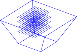
(A) Geometry of the alveolus.

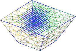
(B) Surface mesh.

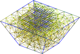
(C) Volume mesh.

Figure 3: Geometry of the alveolus and computational mesh generated using Gmsh. Each layer of 1D lines alternatively represents a set of water injectors or a group of extraction drains for the gas.

5.3 Heuristic evaluation of the unknown constants in the model

The model presented in this paper features a large set of unknown variables (i.e. diffusion coefficients, scaling factors, …) whose role is crucial to obtain realistic simulations. In this section, we propose a first set of values for these parameters that have been heuristically deduced by means of some qualitative and numerical considerations. A major improvement of the model is expected by a more rigorous tuning of these parameters which will be investigated in future works.

Porous medium

The physical and chemical properties of the bioreactor considered as a porous environment have been derived by experimental results in the literature. In particular, we consider a porosity $\Phi=$0.3\text{\,}$$ and a permeability $D=${10}^{-11}\text{\,}\mathrm{m}^{2}$$.

Bacteria and organic carbon

We consider both the concentration of bacteria $b$ and of organic carbon $C^{\textrm{org}}$ as non-dimensional quantities in order to estimate their evolution. Thus we set $b_{0}=1$ and $C^{\textrm{org}}_{0}=1$ and we derive the values $a_{b}=${10}^{-5}\text{\,}\mathrm{m}^{6}\mathrm{k}\mathrm{g}^{-2}\mathrm{d}^{-1}$$ and $c_{b}=1$ respectively for the rate of consumption of the organic carbon and for the rate of reproduction of bacteria. Within this framework and under the optimal conditions of reaction prescribed by (3.1), $C^{\textrm{org}}$ decreases to $2\permil$ of its initial value during the lifetime of the bioreactor whereas bacteria concentration $b$ remains bounded ($b<2b_{0}$).

Temperature

As per experimental data, the optimal temperature for the methanogenic fermentation to take place is $T_{opt}=$35\text{\,}\mathrm{\SIUnitSymbolCelsius}$=$308\text{\,}\mathrm{K}$$ with an admissible variation of temperature of $\pm A_{T}=$20\text{\,}\mathrm{\SIUnitSymbolCelsius}$=$20\text{\,}\mathrm{K}$$ to guarantee the survival of bacteria. The factor $c_{T}$ represents the heat produced per unit of consumed organic carbon and per unit of time and is estimated to $c_{T}=${10}^{2}\text{\,}\mathrm{K}\,\mathrm{m}^{2}\mathrm{d}^{-1}$$. The thermal conductivity of the waste inside the alveolus is fixed at $k_{T}=$9\text{\times}{10}^{-2}\text{\,}\mathrm{m}^{2}\mathrm{d}^{-1}$$. In order to impose realistic boundary conditions for the heat equation, we consider different values for the temperature of the lateral surface of the alveolus $T_{g}=$5\text{\,}\mathrm{\SIUnitSymbolCelsius}$=$278\text{\,}\mathrm{K}$$ and the one of the top geomembrane $T_{m}=$20\text{\,}\mathrm{\SIUnitSymbolCelsius}$=$293\text{\,}\mathrm{K}$$.

Water

The production of methane takes place only when less than $10\%$ of water is present inside the bioreactor. Since the alveolus is completely flooded when $w=$1000\text{\,}\mathrm{k}\mathrm{g}\,\mathrm{m}^{-3}$$, we get that $w_{\text{max}}=$100\text{\,}\mathrm{k}\mathrm{g}\,\mathrm{m}^{-3}$$. The vertical velocity drift due to gravity is estimated from Darcy’s law to the value $\|u_{w}\|=$2.1\text{\,}\mathrm{m}\,\mathrm{d}^{-1}$$ and the diffusion coefficient is set to $k_{w}=$8.6\text{\times}{10}^{-2}\text{\,}\mathrm{m}^{2}\mathrm{d}^{-1}$$.

Phase transition

In order to model the phase transitions, we have to consider the critical values of the pressure associated with evaporation and condensation. The Rankine law for the vapor pressure of water is approximated using the following values: $P_{0}=$133.322\text{\,}\mathrm{Pa}$$, $s_{0}=20.386$ and $s_{1}=5132K$ and its linearization arises when considering $H_{0}=$-9.56\text{\times}{10}^{4}\text{\,}\mathrm{Pa}$$ and $H_{1}=$337.89\text{\,}\mathrm{Pa}\,\mathrm{K}^{-1}$$ for the range of temperatures $[$288\text{\,}\mathrm{K}$;$328\text{\,}\mathrm{K}$]$. Moreover, we set the value $c_{h\to w}$ that represents the speed for the condensation of vapor to liquid water: $c_{h\to w}=${10}^{-1}\text{\,}\mathrm{d}^{-1}$$.

Gases

We consider a gas mixture made of methane, carbon dioxide and water vapor. Its dynamical viscosity is set to $\mu_{\text{gas}}=$1.3\text{\,}\mathrm{P}\mathrm{a}\,\mathrm{d}^{-1}$$. Other parameters involved represent the rate of production of a specific gas (methane, carbon dioxide and water vapor) per unit of consumed organic carbon and per unit of time: $c_{M}=$1.8\text{\times}{10}^{7}\text{\,}\mathrm{k}\mathrm{g}\,\mathrm{m}^{-3}$$; $c_{C}=$2.6\text{\times}{10}^{7}\text{\,}\mathrm{k}\mathrm{g}\,\mathrm{m}^{-3}$$; $c_{h}=$2.5\text{\times}{10}^{6}\text{\,}\mathrm{k}\mathrm{g}\,\mathrm{m}^{-3}$$.

Remark 5.1.

A key aspect in the modeling of a bioreactor landfill is the possibility to adapt the incoming flow of water and leachates $J_{\textrm{in}}$ and the outgoing flow of biogas $J_{\textrm{out}}$. These values are user-defined parameters which are kept constant to $258\text{\,}\mathrm{m}^{3}\,\mathrm{d}^{-1}$ for the simulations in this paper but should act as control variables in the framework of the forecast and optimization procedures described in the introduction.

5.4 A preliminary test case

In this section we present some preliminary numerical results obtained by using the SiViBiR++ module developed in Feel++ to solve the equations presented in section 3 using the numerical schemes discussed in section 4. In particular, we remark that in all the following simulations we neglect the effects due to the gas and fluid dynamics inside the bioreactor landfill. Though this choice limits the ability of the discussed results to correctly describe the complete physical behavior of the system, this simplification is a necessary starting point for the validation of the mathematical model in section 3. As a matter of fact, the equations describing the gas and fluid dynamics feature several unknown parameters whose tuning - independent and coupled with one another - has to be accurately performed before linking them to the problems modeling the consumption of organic carbon and the evolution of the temperature.
Thus, here we restrict our numerical simulations to two main phenomena occurring inside the bioreactor landfill: first, we describe the consumption of organic carbon under some fixed optimal conditions of humidity and temperature; then we introduce the evolution in time of the temperature and we discuss the behavior of the coupled system given by equations (3.5)-(3.6).

The test cases are studied in the computational domain introduced in section 5.2: in particular, we consider the triangulation of mesh size $5\text{\,}\mathrm{m}$ in figure 3C and we set the unit measure for the time evolution to $\Delta t=$365\text{\,}\mathrm{d}$$. The final time for the simulation is $S^{\textrm{fin}}=40$ years. The parameters inside the equations are set according to the values in section 5.3 but a thorough investigation of these quantities has to be performed to verify their accuracy. The computations have been executed using up to $32$ processors and below we present some simulations for the aforementioned preliminary test cases.

Evolution of the organic carbon under optimal hydration and temperature conditions

First of all, we consider the case of a single uncoupled equation, that is the evolution of the organic carbon in a scenario in which the concentration of water and the temperature are fixed. Starting from equation (3.5), we assume fixed optimal conditions for the humidity and the temperature inside the bioreactor landfill. We set a fixed amount of water $w=\frac{w_{\textrm{max}}}{2}$ inside the alveolus and a constant temperature $T=T_{\textrm{opt}}$. Thus, from (3.1) we get

$$\Psi_{1}(w)\equiv\frac{w_{\textrm{max}}}{4},\qquad\Psi_{2}(T)\equiv 1$$

and equation (3.5) reduces to

$$\begin{cases}\displaystyle(1-\phi)\partial_{t}C^{\textrm{org}}(x,t)=-a_{b}\ \frac{w_{\textrm{max}}}{4}[b_{0}+c_{b}(C^{\textrm{org}}_{0}-C^{\textrm{org}}(x,t))]\ C^{\textrm{org}}(x,t)\ ,\ &\text{in }\Omega\times(0,S^{\textrm{fin}}]\\ C^{\textrm{org}}(\cdot,0)=C^{\textrm{org}}_{0}\ ,\ &\text{in }\overline{\Omega}\end{cases}$$ (5.1)

It is straightforward to observe that equation (5.1) only features one unknown variable - namely the organic carbon - since the concentration of bacteria $b(x,t)$ is an affine function of the concentration of organic carbon itself (cf. equation (3.4)).

As stated in section 4.2, the key aspect in the solution of equation (5.1) is the handling of the non-linear reaction term. In order to numerically treat this term as described, at each time step we need the value $C^{\textrm{org}}_{n}$ at the previous iteration to compute the semi-implicit quantity $C^{\textrm{org}}_{n+1}C^{\textrm{org}}_{n}$. To provide a suitable value of $C^{\textrm{org}}_{n}$ during the first iteration, we solve a linearization of equation (5.1) and we use the corresponding solution to evaluate $C^{\textrm{org}}_{n+1}C^{\textrm{org}}_{n}$.
The initial concentration of organic carbon inside the bioreactor is set to $1$ and in figure 4 we observe several snapshots of the quantity of organic carbon inside the alveolus at time $t=1$ year, $t=10$ years, $t=20$ years and $t=40$ years. At the end of the life of the facility, the amount of organic carbon inside the alveolus is $C^{\textrm{org}}=$2.0\text{\times}{10}^{-3}\text{\,}$$.

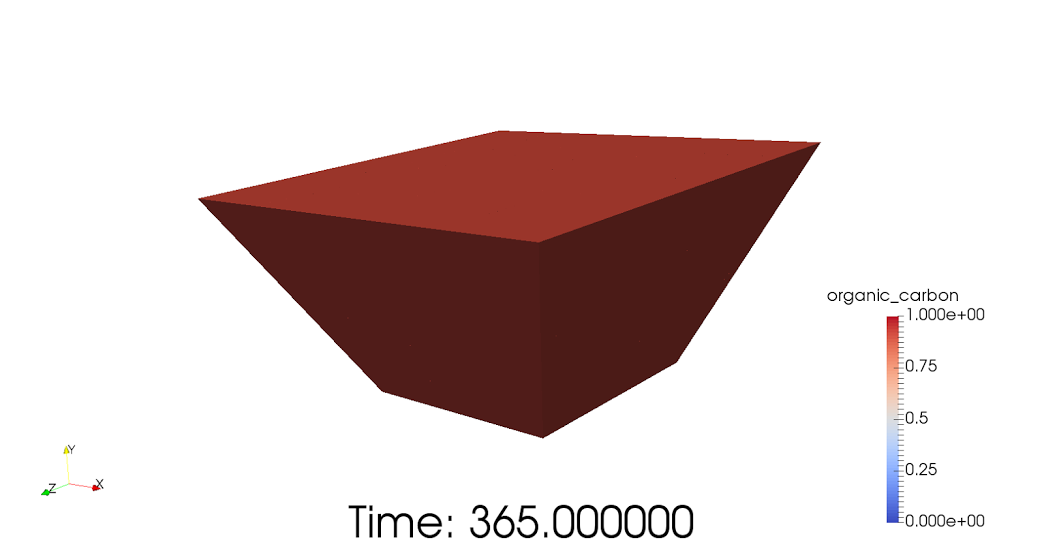
(A) Lifetime: $1$ year.

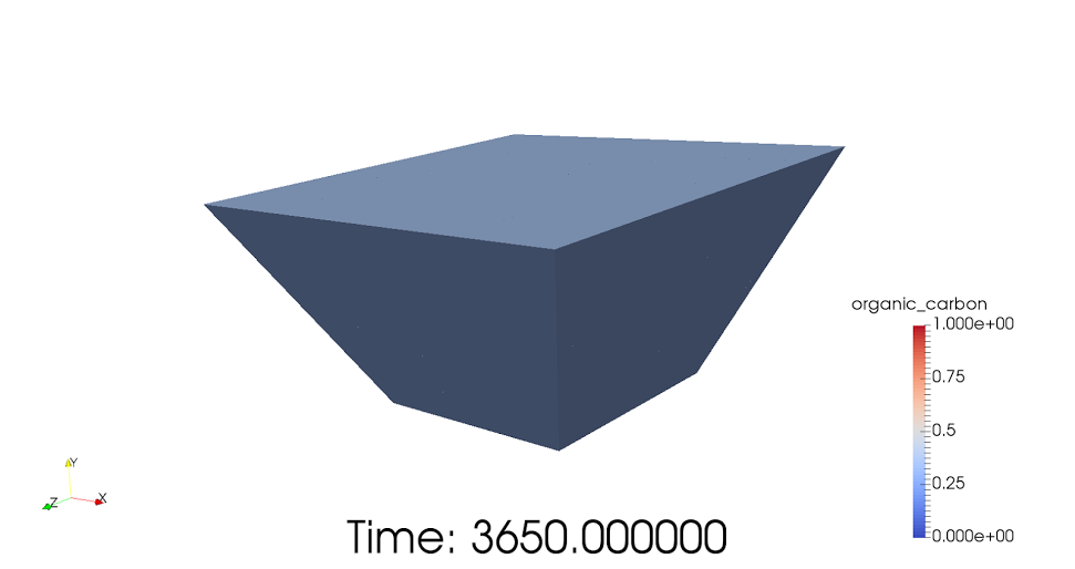
(B) Lifetime: $10$ years.

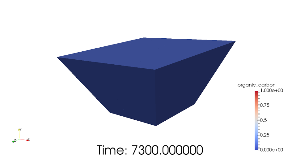
(C) Lifetime: $20$ years.

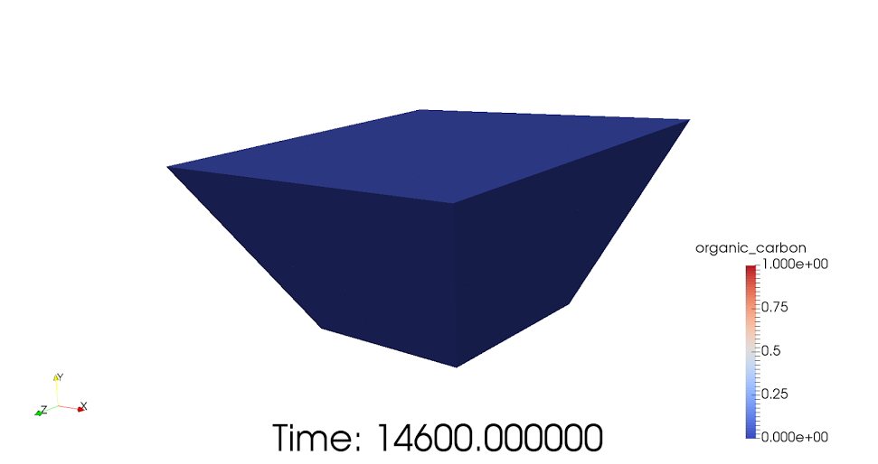
(D) Lifetime: $40$ years.

Figure 4: Evolution of the organic carbon inside the alveolus at $t=1$ year, $t=10$ years, $t=20$ years and $t=40$ years.

In figure 5, we plot the evolution of the overall quantity of organic carbon with respect to time. In particular, as expected we observe that $C^{\textrm{org}}$ decreases in time as the methanogenic fermentation takes place.

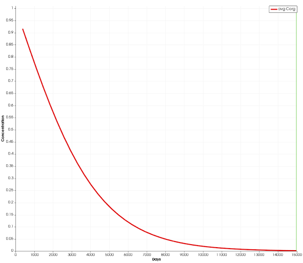
Figure 5: Evolution of the organic carbon between $t=0$ and $t=40$ years under optimal hydration and temperature conditions.

Evolution of the temperature as a function of organic carbon

We introduce a novel variable depending both on space and time to model the temperature inside the bioreactor. Figure 6 presents the snapshots of the value of the temperature in a section of the alveolus under analysis at time $t=1$ year, $t=10$ years, $t=20$ years and $t=40$ years. These result from the solution of equation (3.6) for a given trend of the organic carbon. Let us consider the evolution of the organic carbon obtained from the previous test case. The corresponding profile is given by

$$C^{\textrm{org}}(x,t)=e^{-\alpha t}\qquad,\qquad\alpha=${10}^{-3}\text{\,}$.$$

We observe that the consumption of organic carbon by means of the chemical reaction (2.2) is responsible for the generation of heat in the middle of the domain. As expected by the physics of the problem, the heat tends to diffuse towards the external boundaries where the temperature is lower.

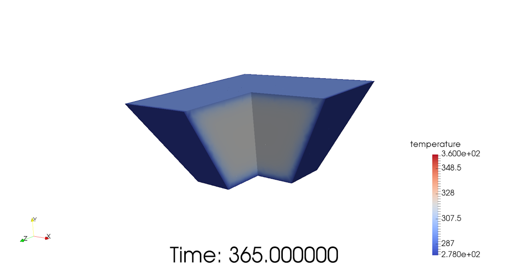
(A) Lifetime: $1$ year.

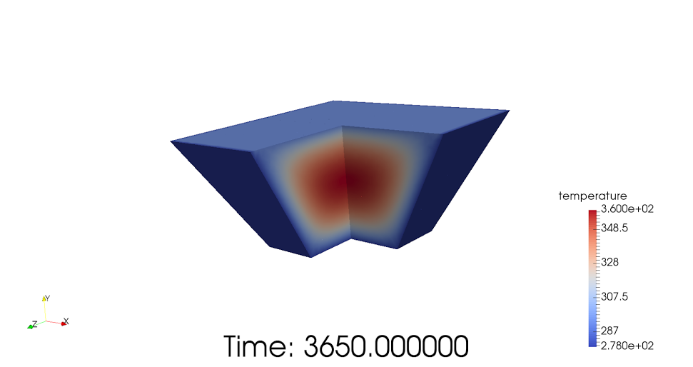
(B) Lifetime: $10$ years.

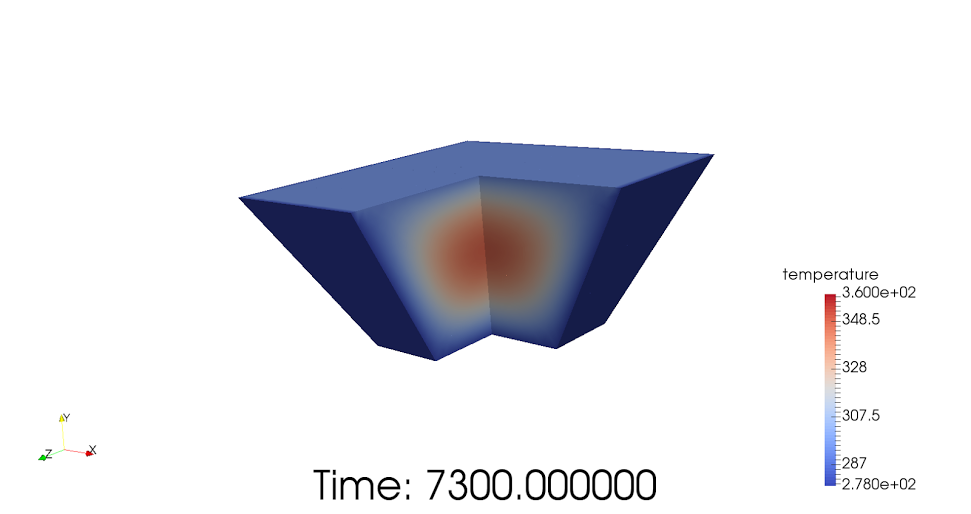
(C) Lifetime: $20$ years.

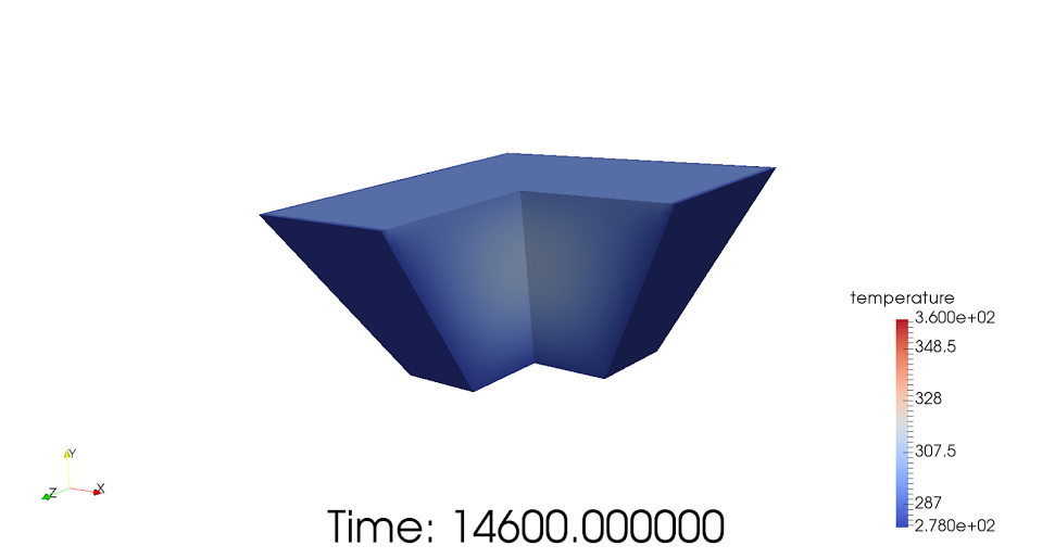
(D) Lifetime: $40$ years.

Figure 6: Evolution of the temperature inside the alveolus at $t=1$ year, $t=10$ years, $t=20$ years and $t=40$ years.

After a first phase which lasts approximately $10$ years in which the methanogenic process produces heat and the temperature rises, the consumption of organic carbon slows down and the temperature as well starts to decrease until the end-of-life of the facility (Fig. 7A-7B).

(A) Evolution of the organic carbon.

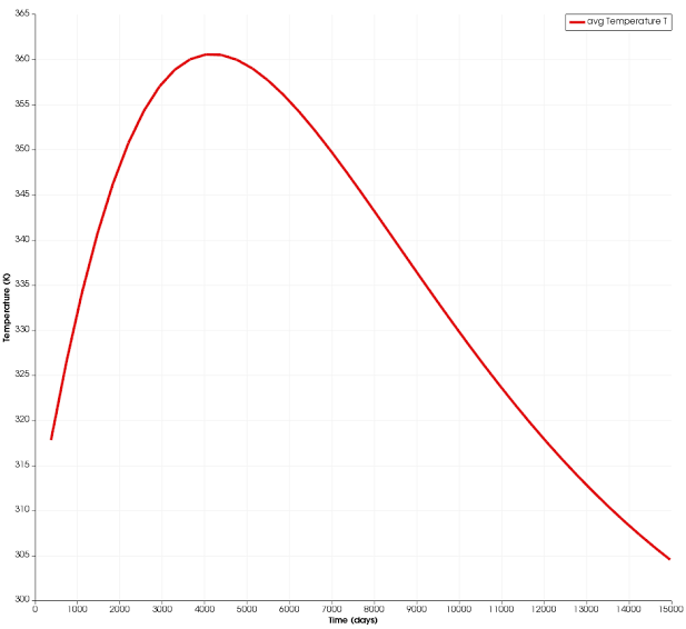
(B) Evolution of the temperature.

Figure 7: Evolution of the quantity of organic carbon and temperature inside the alveolus between $t=0$ and $t=40$ years.

Evolution of the coupled system of organic carbon and temperature under optimal hydration condition

Starting from the previously discussed cases, we now proceed to the coupling of the organic carbon with the temperature. We keep the optimal hydration condition as in the previous simulations - that is $w=\frac{w_{\textrm{max}}}{2}$ - and we consider the solution of the coupled equations (3.5)-(3.6).

From the numerical point of view, this scenario introduces several difficulties, mainly due to the fact that the two equations are now dependent on one another. As mentioned in section 4, the coupling is handled explicitly, that is, first we solve the problem featuring the organic carbon with fixed temperature then we approximate the heat equation using the information arising from the previously computed $C^{\textrm{org}}$.
Within this framework, at time $t=t_{n}$ the conditions of humidity and temperature for the organic carbon equation read as

$$\Psi_{1}(w)\equiv\frac{w_{\textrm{max}}}{4},\qquad\Psi_{2}(T)=\max\left(0,1-\frac{|T_{n}-T_{\textrm{opt}}|}{A_{T}}\right)$$

where $T_{n}$ is the temperature at the previous iteration.

As in the previous case, we consider an initial concentration of organic carbon equal to $1$ and we observe it decreasing in figure 8A due to the bacterial activity. We verify that the quantity of organic carbon inside the bioreactor landfill decays towards zero during the lifetime of the facility. At the same time, the temperature increases as a result of the methanogenic process catalyzed by the microbiota (Fig. 8B). Nevertheless, when the temperature goes beyond the tolerated variation $A_{T}$, the second condition in (3.1) is no more fulfilled and the chemical reaction is prevented.

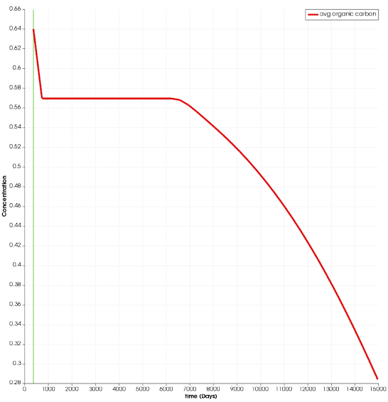
(A) Evolution of the organic carbon.

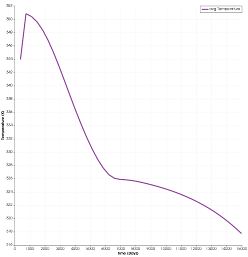
(B) Evolution of the temperature.

Figure 8: Evolution of the quantity of organic carbon and the temperature inside the alveolus between $t=0$ and $t=40$ years.

We may observe this behavior in figures 8A-8B between $t=3$ years and $t=20$ years. Once the temperature is inside the admissible range $[T_{\textrm{opt}}-A_{T};T_{\textrm{opt}}+A_{T}]$ again (starting approximately from $t=20$ years), the reaction (2.2) is allowed, the organic carbon is consumed and influences the temperature which slightly increases again before eventually decreasing towards the end-of-life of the bioreactor.

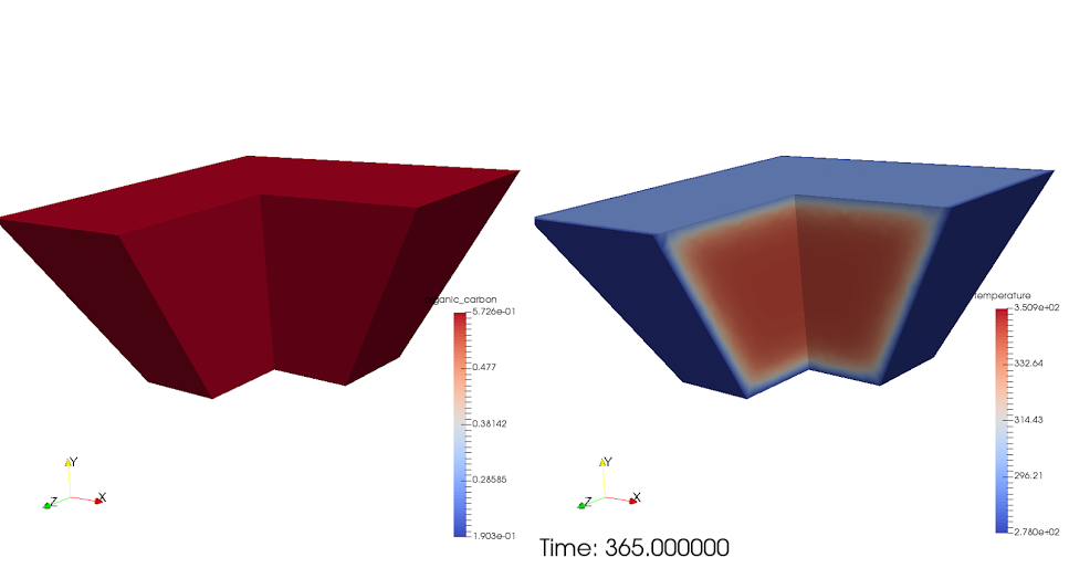
(A) Lifetime: $1$ year.

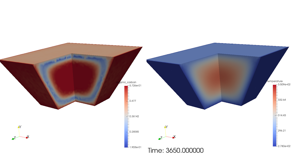
(B) Lifetime: $10$ years.

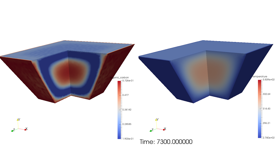
(C) Lifetime: $20$ years.

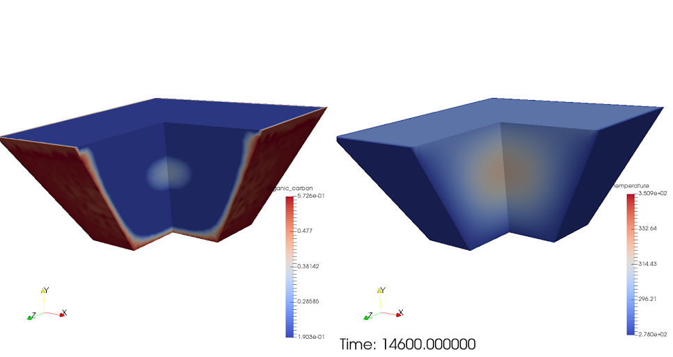
(D) Lifetime: $40$ years.

Figure 9: Coupled evolution of the organic carbon (left) and the temperature (right) inside the alveolus at $t=1$ year, $t=10$ years, $t=20$ years and $t=40$ years.

Eventually, in figure 9 we report some snapshots of the solutions of the coupled system (3.5)-(3.6).

6 Conclusion

In this work, we proposed a first attempt to mathematically model the physical and chemical phenomena taking place inside a bioreactor landfill. A set of $7$ coupled equations has been derived and a Finite Element discretization has been introduced using Feel++. A key aspect of the discussed model is the tuning of the coefficients appearing in the equations. On the one hand, part of these unknowns represents physical quantities whose values may be derived from experimental studies. On the other hand, some parameters are scalar factors that have to be estimated by means of heuristic approaches. A rigorous tuning of these quantities represents a major line of investigation to finalize the implementation of the model in the SiViBiR++ module and its validation with real data.

The present work represents a starting point for the development of mathematically-sound investigations on bioreactor landfills. From a modeling point of view, some assumptions may be relaxed, for example by adding a term to account for the death rate of bacteria or the cooling effect due to water injection inside the bioreactor. The final goal of SiViBiR++ project is the simulation of long-time behavior of the bioreactor in order to perform forecasts on the methane production and optimize the control strategy. The associated inverse problems and PDE-constrained optimization problems are likely to be numerically intractable due to their complexity and their dimension thus the study of reduced order models may be necessary to decrease the overall computational cost.

Appendix A Summary of the unknown parameters

In the following table, we summarize the values of some unknown parameters which were deduced during the present work. We highlight that all these quantities have been estimated via heuristic approaches and a rigorous verification/validation procedure remains necessary before their application to real-world problems.

Table 1: Summary of the parameters involved in the $7$-equations model.

Parameter	Description	Value	Unit
$\Phi$	Porosity of the medium	$0.3\text{\,}$
$D$	Permeability	${10}^{-11}\text{\,}$	$\text{\,}\mathrm{m}^{2}$
$b_{0}$	Initial concentration of bacteria	$1.0\text{\,}$
$C^{\textrm{org}}_{0}$	Initial concentration of organic carbon	$1.0\text{\,}$
$a_{b}$	Rate of consumption of organic carbon	${10}^{-5}\text{\,}$	$\text{\,}\mathrm{m}^{6}\mathrm{k}\mathrm{g}^{-2}\mathrm{d}^{-1}$
$c_{b}$	Rate of creation of bacteria	$1.0\text{\,}$
$T_{\textrm{opt}}$	Optimal temperature for the reaction	$308\text{\,}$	$\text{\,}\mathrm{K}$
$A_{T}$	Tolerated variation of temperature	$20\text{\,}$	$\text{\,}\mathrm{K}$
$c_{T}$	Rate of production of heat by the chemical reaction	${10}^{2}\text{\,}$	$\text{\,}\mathrm{K}$
$k_{T}$	Thermal conductivity	$9\text{\times}{10}^{-2}\text{\,}$	$\text{\,}\mathrm{m}^{2}\mathrm{d}^{-1}$
$T_{g}$	Temperature of the soil	$278\text{\,}$	$\text{\,}\mathrm{K}$
$T_{m}$	Temperature of the geomembrane	$293\text{\,}$	$\text{\,}\mathrm{K}$
$T_{0}$	Initial temperature	$293\text{\,}$	$\text{\,}\mathrm{K}$
$w_{\textrm{max}}$	Maximal admissible quantity of water	$100\text{\,}$	$\text{\,}\mathrm{k}\mathrm{g}\,\mathrm{m}^{-3}$
$\|u_{w}\|$	Velocity of the water	$2.1\text{\,}$	$\text{\,}\mathrm{m}\,\mathrm{d}^{-1}$
$k_{w}$	Diffusion coefficient of the water	$8.6\text{\times}{10}^{-2}\text{\,}$	$\text{\,}\mathrm{m}^{2}\mathrm{d}^{-1}$
$w_{0}$	Initial quantity of water	$50\text{\,}$	$\text{\,}\mathrm{k}\mathrm{g}\,\mathrm{m}^{-3}$
$H_{0}$	Constant for the vapor pressure	$-9.56\text{\times}{10}^{4}\text{\,}$	$\text{\,}\mathrm{Pa}$
$H_{1}$	Constant for the vapor pressure	$337.89\text{\,}$	$\text{\,}\mathrm{Pa}\,\mathrm{K}^{-1}$
$c_{h\to w}$	Condensation rate	${10}^{-1}\text{\,}$	$\text{\,}\mathrm{d}^{-1}$
$\mu_{\text{gas}}$	Dynamical viscosity of the gas	$1.3\text{\,}$	$\text{\,}\mathrm{P}\mathrm{a}\,\mathrm{d}^{-1}$
$c_{M}$	Rate of production of methane	$1.8\text{\times}{10}^{7}\text{\,}$	$\text{\,}\mathrm{k}\mathrm{g}\,\mathrm{m}^{-3}$
$c_{C}$	Rate of production of carbon dioxide	$2.6\text{\times}{10}^{7}\text{\,}$	$\text{\,}\mathrm{k}\mathrm{g}\,\mathrm{m}^{-3}$
$c_{h}$	Rate of production of water vapor	$2.5\text{\times}{10}^{6}\text{\,}$	$\text{\,}\mathrm{k}\mathrm{g}\,\mathrm{m}^{-3}$
$M_{0}$	Initial concentration of methane	$1.0\text{\,}$
$C^{\textrm{dx}}_{0}$	Initial concentration of carbon dioxide	$1.0\text{\,}$
$h_{0}$	Initial concentration of water vapor	$1.0\text{\,}$
$J_{\textrm{out}}$	Outgoing flow of biogas	$258\text{\,}$	$\text{\,}\mathrm{m}^{3}\mathrm{d}^{-1}$
$J_{\textrm{in}}$	Incoming flow of water and leachates	$258\text{\,}$	$\text{\,}\mathrm{m}^{3}\mathrm{d}^{-1}$

Acknowledgments

The authors are grateful to Alexandre Ancel (Université de Strasbourg) and the Feel++ community for the technical support. The authors wish to thank the CEMRACS 2015 and its organizers.

References

- [1] F. Agostini, C. Sundberg, and R. Navia. Is biodegradable waste a porous environment? A review. Waste Manage. Res., 30(10):1001–1015, 2012.
- [2] S. Balay, S. Abhyankar, M. Adams, J. Brown, P. Brune, K. Buschelman, L. Dalcin, V. Eijkhout, W. Gropp, D. Karpeyev, D. Kaushik, M. Knepley, L. Curfman McInnes, K. Rupp, B. Smith, S. Zampini, and H. Zhang. PETSc Users Manual. Technical report, Argonne National Laboratory, 2015.
- [3] F. Bezzo, S. Macchietto, and C. C. Pantelides. General hybrid multizonal/CFD approach for bioreactor modeling. AIChE Journal, 49(8):2133–2148, 2003.
- [4] P. B. Bochev, M. D. Gunzburger, and J. N. Shadid. Stability of the SUPG finite element method for transient advection-diffusion problems. Comput. Method. Appl. M., 193(23-26):2301–2323, 2004.
- [5] D. Boffi, F. Brezzi, and M. Fortin. Mixed finite element methods and applications, volume 44 of Springer Series in Computational Mathematics. Springer, Heidelberg, 2013.
- [6] E. Burman. Consistent SUPG-method for transient transport problems: Stability and convergence. Comput. Method. Appl. M., 199(17-20):1114–1123, 2010.
- [7] V. Chabanne. Vers la simulation des écoulements sanguins. Ph.D. thesis, Université Joseph Fourier, Grenoble, 2013.
- [8] T. Chassagnac. Etat des connaissances techniques et recommandantions de mise en oeuvre pour une gestion des installations de stockage de déchets non dangereux en mode bioréacteur. Technical report, ADEME - Agence Nationale de l’Environnement et de la Maîtrise de l’Energie. FNADE - Fédération Nationale des Activités de la Dépollution et de l’Environnement, 2007.
- [9] A. J. Chorin and J. E. Marsden. A mathematical introduction to fluid mechanics, volume 4 of Texts in Applied Mathematics. Springer-Verlag, New York, third edition, 1993.
- [10] D. Córdoba, F. Gancedo, and R. Orive. Analytical behavior of two-dimensional incompressible flow in porous media. J. Math. Phys., 48(6):065206, 2007.
- [11] M. R. Correa and A. F. D. Loula. Unconditionally stable mixed finite element methods for Darcy flow. Comput. Method. Appl. M., 197(17-18):1525–1540, 2008.
- [12] L. J. Durlofsky. Accuracy of mixed and control volume finite element approximations to Darcy velocity and related quantities. Water Resour. Res., 30(4):965–973, 1994.
- [13] C. Geuzaine and J.-F. Remacle. Gmsh: a three-dimensional finite element mesh generator with built-in pre- and postprocessing facilities, 2009.
- [14] C. Johnson et al. Characterization, Design, Construction and Monitoring of Bioreactor Landfills. Technical report, ITRC - Interstate Technology & Regulatory Council, 2006.
- [15] C. Johnson, U. Nävert, and J. Pitkäranta. Finite element methods for linear hyperbolic problems. Comput. Method. Appl. M., 45(1):285–312, 1984.
- [16] J. Kindlein, D. Dinkler, and H. Ahrens. Numerical modelling of multiphase flow and transport processes in landfills. Waste Manage. Res., 24(4):376–387, 2006.
- [17] T. Kling and J. Korkealaakso. Multiphase modeling and inversion methods for controlling landfill bioreactor. In Proceedings of TOUGH Symposium. Lawrence Berkeley National Laboratory, Berkeley, CA, USA, 2006.
- [18] M. Lebeau and J.-M. Konrad. Natural convection of compressible and incompressible gases in undeformable porous media under cold climate conditions. Comput. Geotech., 36(3):435–445, 2009.
- [19] C. N. Liu, R. H. Chen, and K. S. Chen. Unsaturated consolidation theory for the prediction of long-term municipal solid waste landfill settlement. Waste Manage. Res., 24(1):80–91, 2006.
- [20] S. Martín, E. Marañón, and H. Sastre. Mathematical modelling of landfill gas migration in MSW sanitary landfills. Waste Manage. Res., 19(5):425–435, 2001.
- [21] P. McCreanor. Landfill leachate recirculation systems: Mathematical modelling and validation. PhD thesis, University of Central Florida, USA, 1998.
- [22] C. Prud’homme. A Domain Specific Embedded Language in C++ for automatic differentiation, projection, integration and variational formulations. Sci. Program., 14(2):81–110, 2006.
- [23] C. Prud’homme, V. Chabannes, V. Doyeux, M. Ismail, A. Samake, and G. Pena. Feel++: A computational framework for Galerkin methods and advanced numerical methods. ESAIM: ProcS, 38:429–455, 2012.
- [24] P. A. Raviart and J. M. Thomas. A mixed finite element method for second order elliptic problems. In I. Galligani and E. Magenes, editors, Mathematical Aspects of Finite Element Methods, volume 606 of Lect. Notes Math, pages 292–315. Springer-Verlag, 1977.
- [25] D. R. Reinhart and B. A. Al-Yousfi. The impact of leachate recirculation on municipal solid waste landfill operating characteristics. Waste Manage. Res., 14(4):337–346, 1996.
- [26] H. S. Sidhu, M. I. Nelson, and X. D. Chen. A simple spatial model for self-heating compost piles. In W. Read and A. J. Roberts, editors, Proceedings of the 13th Biennial Computational Techniques and Applications Conference, CTAC-2006, volume 48 of ANZIAM J., pages C135–C150, 2007.
- [27] K. Vafai. Handbook of porous media. Crc Press, 2015.
- [28] J. J. Walsh and R. N. Kinman. Leachate and gas production under controlled moisture conditions. In Municipal Solid Waste: Land Disposal, Proceedings of the 5th Annual Research Symposium, pages 41–57. EPA-600/9-79-023a, 1979.