canonical contact unit cotangent bundle

Abstract.

We describe an explicit open book decomposition adapted to the canonical contact structure on the unit cotangent bundle of a closed surface.

1. Introduction

Let $S$ denote a closed surface which is not necessarily orientable. Let $\pi$ denote the projection of the bundle of cooriented lines tangent to $S$ onto $S$. For a point $q\in S$ and a cooriented line $u$ in $T_{q}S$, let $\xi_{(q,u)}$ denote the cooriented plane described uniquely by the equation $\pi_{*}(\xi_{(q,u)})=u\in T_{q}S$. The canonical contact structure $\xi_{can}$ on the bundle of cooriented lines tangent to $S$ consists of these planes (see, for example, [15]).

If $S$ is equipped with a Riemannian metric, then the bundle of cooriented lines tangent to $S$ can be identified with the unit cotangent bundle $ST^{*}S$, and $\xi_{can}$ is given by the kernel of the Liouville $1$-form $\lambda_{can}$ under this identification. Moreover, the disk cotangent bundle $DT^{*}S$ equipped with its canonical symplectic structure $\omega_{can}=d\lambda_{can}$ is a minimal strong symplectic filling of the contact $3$-manifold $(ST^{*}S,\xi_{can})$.

In this article, we describe an explicit abstract open book decomposition adapted to the contact $3$-manifold $(ST^{*}S,\xi_{can})$, in the sense of Giroux [10]. In the following, we use $\Sigma_{g}$ to denote the orientable closed surface of genus $g$ and $N_{k}$ to denote the non-orientable closed surface obtained by the connected sum of $k$ copies of the real projective plane $\mathbb{RP}^{2}$.

In Theorem 3.1 (resp. Theorem 3.4), for any $g\geq 1$, we describe an open book adapted to $(ST^{*}\Sigma_{g},\xi_{can})$, whose page is a genus $g$ surface with $2g+2$ (resp. $g+2$) boundary components and we give an explicit factorization of its monodromy into a product of positive Dehn twists. In Corollary 3.5, we also describe an exact symplectic Lefschetz fibration over $D^{2}$, whose total space is symplectomorphic to $(DT^{*}\Sigma_{g},\omega_{can})$, up to completion.

In Theorem 3.7, for any $k\geq 1$, we describe an open book adapted to $(ST^{*}N_{k},\xi_{can})$, whose page is a planar surface with $2k+2$ boundary components and we give an explicit factorization of its monodromy into a product of positive Dehn twists.

The unit cotangent bundle $ST^{*}\Sigma_{0}$ is diffeomorphic to the real projective space $\mathbb{RP}^{3}$, and $\xi_{can}$ is the unique tight contact structure in $\mathbb{RP}^{3}$, up to isotopy (cf. [12]). It is well-known (see, for example [8]) that $(\mathbb{RP}^{3},\xi_{can})$ has an adapted open book whose page is the annulus and whose monodromy is the square of the positive Dehn twist along the core circle of the annulus. Moreover, McDuff [17] showed that any minimal symplectic filling of $(\mathbb{RP}^{3},\xi_{can})$ is diffeomorphic to $DT^{*}\Sigma_{0}$.

The unit cotangent bundle $ST^{*}\Sigma_{1}$ is diffeomorphic to the $3$-torus $T^{3}$ and Eliashberg [5] showed that $\xi_{can}$ is the unique strongly symplectically fillable contact structure in $T^{3}$, up to contactomorphism. In his thesis [22], Van Horn-Morris constructed an explicit open book with genus one pages adapted to $(T^{3},\xi_{can})$. Note that $(T^{3},\xi_{can})$ can not be supported by a planar open book by a theorem of Etnyre [7]. Moreover, according to Wendl [24], any minimal strong symplectic filling of $(T^{3},\xi_{can})$ is symplectic deformation equivalent to $(DT^{*}\Sigma_{1}\cong T^{2}\times D^{2},\omega_{can})$.

The unit cotangent bundle $ST^{*}N_{1}$ is diffeomorphic to the lens space $L(4,1)$ and $\xi_{can}$ is the unique universally tight contact structure in $L(4,1)$, up to contactomorphism. Note that the canonical contact structure on $L(4,1)$ viewed as a singularity link is isomorphic to $\xi_{can}$ defined as above. It is well-known (see, for example [8]) that $(L(4,1),\xi_{can})$ has an adapted open book whose page is the 4-holed sphere and whose monodromy is the product of positive Dehn twists along four curves each of which is parallel to a boundary component. Moreover, McDuff [17] showed that $(L(4,1),\xi_{can})$ has two minimal symplectic fillings up to diffeomorphism: (i) the disk cotangent bundle $DT^{*}N_{1}$, which is a rational homology $4$-ball and (ii) the disk bundle over the sphere with Euler number $-4$.

We would like to point out that in an unpublished expository article [16], Massot argues that, for all $g\geq 2$, the contact $3$-manifold $(ST^{*}\Sigma_{g},\xi_{can})$ has an adapted open book with genus one pages but he does not describe its monodromy. The interested reader can turn to [4] and [9] for related material.

2. Exact symplectic Lefschetz fibrations

Suppose that $W$ is a smooth $4$-manifold with nonempty boundary equipped with an exact symplectic form $\omega=d\alpha$ such that the Liouville vector field, which is by definition $\omega$-dual to $\alpha$, is transverse to $\partial W$ and points outwards. Then $(W,\omega)$ is called an exact symplectic $4$-manifold with $\omega$-convex boundary and it is also called an exact symplectic filling of the contact $3$-manifold $(\partial W,\ker(\alpha|_{\partial W}))$ if the contact boundary is desired to be emphasized.

The definition above can be extended to smooth manifolds with corners as follows (cf. [21, Section 7a]). Let $W$ be a smooth $4$-manifold with codimension $2$ corners. An exact symplectic structure on $W$ is given by a symplectic $2$-form $\omega=d\alpha$ on $W$ such that the Liouville vector field (again defined as $\omega$-dual to $\alpha$) is transverse to each boundary stratum of codimension $1$ and points outwards. It follows that $\alpha$ induces a contact form on each boundary stratum. Moreover, if the corners of $W$ are rounded off (see [21, Lemma 7.6]), it becomes an exact symplectic filling of its contact boundary.

Definition 2.1.

An exact symplectic Lefschetz fibration on an exact symplectic $4$-manifold $(W,\omega)$ with codimension $2$ corners is a smooth map $\pi:(W,\omega)\to D^{2}$ satisfying the following conditions:

• The map $\pi$ has finitely many critical points $p_{1},\ldots,p_{k}$ in the interior of $W$ such that around each critical point, $\pi$ is modeled on the map $(z_{1},z_{2})\to z_{1}^{2}+z_{2}^{2}$ in complex local coordinates compatible with the orientations.

• Every fiber of the map $\pi|_{W\setminus\{p_{1},\ldots,p_{k}\}}:W\setminus\{p_{1},\ldots,p_{k}\}\to D^{2}$ is a symplectic submanifold.

• $\partial W$ consists of two smooth boundary strata $\partial_{v}W$ (the vertical boundary) and $\partial_{h}W$(the horizontal boundary) meeting at a codimension $2$ corner, where

  $$\partial_{v}W=\pi^{-1}(\partial D^{2})\;\mbox{and}\;\partial_{h}W=\bigcup_{z\in D^{2}}\partial(\pi^{-1}(z)).$$

  We require that $\pi|_{\partial_{v}W}:\partial_{v}W\to\partial D^{2}$ is smooth fibration and $\pi$ is a trivial smooth fibration over $D^{2}$ near $\partial_{h}W$.

The vertical boundary $\partial_{v}W$ is a surface fibration over the circle and the horizontal boundary $\partial_{h}W$ is a disjoint union of some number of copies of $S^{1}\times D^{2}$. The vertical and horizontal boundaries meet each other at the corner

$$\partial_{v}W\cap\partial_{h}W=\partial(\partial_{h}W)=\coprod(S^{1}\times\partial D^{2}).$$

Therefore, after rounding off the corners of $W$, its boundary $\partial W$ acquires an open book decomposition given by $\pi|_{\partial W\setminus B}:\partial W\setminus B\to\partial D^{2}$, where $\partial_{h}W$ is viewed as a tubular neighborhood of the binding $B:=\coprod(S^{1}\times\{0\})$. Moreover, $\alpha$ restricts to a contact form on $\partial W$ whose kernel is a contact structure supported by this open book.

Remark 2.2.

A smooth Lefschetz fibration on a smooth $4$-manifold $W$ with codimension $2$ corners, is a smooth map $\pi:W\to D^{2}$ which satisfies the first and the last conditions listed in the Definition 2.1.

Next, we briefly recall (see [21, Section 16], [11, Chapter 8]) how the topology of the total space of an exact symplectic Lefschetz fibration

$$\pi:(W,\omega)\to D^{2}$$

is described using a distinguished basis of vanishing paths in $D^{2}$.

Without loss of generality, we can assume that $D^{2}$ is the unit disk $\mathbb{D}$ in $\mathbb{C}$. For each critical value $z\in\mathbb{D}$ of the fibration $\pi$, the fiber $\pi^{-1}(z)$ is called a singular fiber, while the other fibers are called regular. Throughout this paper, we will assume that a regular fiber is connected and each singular fiber contains a unique critical point. By setting $z_{0}=1\in\partial\mathbb{D}$, the regular fiber $F=\pi^{-1}(z_{0})$, which is a symplectic submanifold of $(W,\omega)$, serves as a reference fiber in the discussion below. We call $z_{0}$ the base point.

For any critical value $z\in int\;\mathbb{D}$, a vanishing path is an embedded path $\gamma:[0,1]\to\mathbb{D}$ such that $\gamma(0)=z_{0}$ and $\gamma(1)=z\in\mathbb{D}$. To each such path, one can associate its Lefschetz thimble $\Delta_{\gamma}$, which the unique embedded Lagrangian disk in $(W,\omega)$ such that $\pi(\Delta_{\gamma})=\gamma([0,1])$ and $\pi(\partial\Delta_{\gamma})=z_{0}$. The boundary $\partial\Delta_{\gamma}$ of the Lefschetz thimble is therefore an (exact) Lagrangian circle in $(F,\omega|_{F})$. This circle is called a vanishing cycle since under a parallel transport along $\gamma$, it collapses to the unique singular point on the fiber $\pi^{-1}(z)$.

A distinguished basis of vanishing paths is an ordered set of vanishing paths $(\gamma_{1},\ldots,\gamma_{k})$ (one for each critical value of $\pi$) starting at the base point $z_{0}$ and ending at a critical value such that $\gamma_{i}$ intersects $\gamma_{j}$ only at $z_{0}$ for $i\neq j$. Note that there is a natural counterclockwise ordering of these paths, by assuming that the starting directions of the paths are pairwise distinct. Let $\delta_{i}$ denote the vanishing cycle in $F$ corresponding to the vanishing path $\gamma_{i}$, whose end point—a critical value—is labeled as $z_{i}$.

Now consider a small loop, oriented counterclockwise, around the critical value $z_{i}$, and connect it to the base point $z_{0}$ using the vanishing path $\gamma_{i}$. One can consider this loop as a loop $a_{i}$ around $z_{i}$ passing through $z_{0}$ and not including any other critical values in its interior. It is a classical fact that $\pi^{-1}(a_{i})$ is a surface bundle over $a_{i}$, which is diffeomorphic to

$$(F\times[0,1])/((x,1)\sim(D(\delta_{i})(x),0)$$

where $D(\delta_{i})$ denotes the positive Dehn twist along the vanishing cycle $\delta_{i}\subset F$.

Similarly, $\pi^{-1}(\partial\mathbb{D})$ is an $F$-bundle over $\mathbb{S}^{1}=\partial\mathbb{D}$ which is diffeomorphic to

$$(F\times[0,1])/((x,1)\sim(\psi(x),0)$$

for some self-diffeomorphism $\psi$ of the fiber $F$ preserving $\partial F$ pointwise. The map $\psi$ is called the geometric monodromy and computed via parallel transport using any choice of a connection on the bundle. Note that the isotopy class of $\psi$ is independent of the choice of the connection. It follows that

$$\psi=D(\delta_{k})D(\delta_{k-1})\cdots D(\delta_{1})\in Map(F,\partial F),$$

where $Map(F,\partial F)$ denotes the mapping class group of the surface $F$. The product of positive Dehn twists above is called a monodromy factorization or a positive factorization of the monodromy $\psi$ of the Lefschetz fibration $\pi$.

Note that the vanishing cycle for each singular fiber is determined by the choice of a vanishing path ending at the corresponding critical value. Therefore a different basis of vanishing paths (with the same rules imposed as above) induce a different factorization of the monodromy $\psi$. Nevertheless, any two distinguished bases of vanishing paths are related by a sequence of transformations—the Hurwitz moves. An elementary Hurwitz move is obtained by switching the order of two consecutive vanishing paths as shown in Figure 1 keeping the other vanishing paths fixed. This will have the following affect on the ordered set of vanishing cycles

$$(\delta_{1},\ldots,\delta_{i-1},\delta_{i},\delta_{i+1},\delta_{i+2},\ldots,\delta_{k})\to(\delta_{1},\ldots,\delta_{i-1},\delta_{i+1},D(\delta_{i+1})(\delta_{i}),\delta_{i+2},\ldots,\delta_{k}),$$

which is also called an elementary Hurwitz move. In general a Hurwitz move is any composition of elementary Hurwitz moves and their inverses.

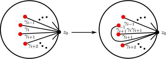
Figure 1. An elementary Hurwitz move

If one chooses a different base point on $\partial\mathbb{D}$ to begin with, then the monodromy of the Lefschetz fibration takes the form $\varphi\psi\varphi^{-1}$, where $\varphi$ is the appropriate element of $Map(F,\partial F)$, obtained by parallel transport. In this case, the monodromy factorization appears as

$$\varphi\psi\varphi^{-1}=\varphi\big{(}D(\delta_{k})D(\delta_{k-1})\cdots D(\delta_{1})\big{)}\varphi^{-1}$$

$$=\varphi D(\delta_{k})\varphi^{-1}\varphi D(\delta_{k-1})\varphi^{-1}\varphi\cdots\varphi^{-1}\varphi D(\delta_{1})\varphi^{-1}$$

$$=D(\varphi(\delta_{k}))D(\varphi(\delta_{k-1}))\cdots D(\varphi(\delta_{1})),$$

where the last equality follows by the fact that the conjugation $\varphi D(\delta)\varphi^{-1}$ of a positive Dehn twist $D(\delta)$ is isotopic to the positive Dehn twist $D(\varphi(\delta))$.

Conversely (cf. [21, Lemma 16.9]),

Lemma 2.3.

Let $(\delta_{1},\ldots,\delta_{k})$ be an ordered collection of embedded (Lagrangian) circles on an exact symplectic surface $F$ with nonempty boundary. Choose a base point $*$ on $\partial D^{2}$, and a distinguished basis of vanishing paths $(\gamma_{1},\ldots,\gamma_{k})$ starting at $*$. Then there is an exact symplectic Lefschetz fibration $\pi:(W,\omega)\to D^{2}$ whose critical values are $\gamma_{1}(1),\ldots,\gamma_{k}(1)$, under which $\delta_{i}$ corresponds to the vanishing cycle for the path $\gamma_{i}$, where $\pi^{-1}(*)=F$ as symplectic manifolds. Moreover, this fibration is trivial near $\partial_{h}W$.

Definition 2.4.

A conformal exact symplectomorphism between two exact symplectic $4$-manifolds $(W_{1},\omega_{1}=d\alpha_{1})$ and $(W_{1},\omega_{2}=d\alpha_{2})$ is a diffeomorphism $\phi:W_{1}\to W_{2}$ such that $\phi^{*}\alpha_{2}=K\alpha_{1}+df$ for some smooth function $f:W_{1}\to\mathbb{R}$, and some real number $K>0$. If $K=1$, then $\phi$ is called an exact symplectomorphism.

Remark 2.5.

The definition above also applies to maps between exact symplectic $4$-manifolds with codimension $2$ corners.

Lemma 2.6.

Suppose that $\pi:(W,\omega)\to D^{2}$ is an exact symplectic Lefschetz fibration whose ordered set of vanishing cycles is given by

$$(\delta_{1},\ldots,\delta_{i-1},\delta_{i},\delta_{i+1},\delta_{i+2},\ldots,\delta_{k})$$

with respect to some distinguished basis of vanishing paths. Then there is an exact symplectic Lefschetz fibration $\widetilde{\pi}:(\widetilde{W},\widetilde{\omega})\to D^{2}$ whose ordered set of vanishing cycles is given by

$$(\delta_{1},\ldots,\delta_{i-1},\delta_{i+1},D(\delta_{i+1})(\delta_{i}),\delta_{i+2},\ldots,\delta_{k})$$

with respect to some distinguished basis of vanishing paths, such that $\pi$ and $\widetilde{\pi}$ are isomorphic through an exact symplectomorphism $\phi:(W,\omega)\to(\widetilde{W},\widetilde{\omega})$.

Proof.

By Lemma 2.3, there is an exact symplectic Lefschetz fibration $\widetilde{\pi}:(\widetilde{W},\widetilde{\omega})\to D^{2}$ whose ordered set of vanishing cycles is given by

$$(\delta_{1},\ldots,\delta_{i-1},\delta_{i+1},D(\delta_{i+1})(\delta_{i}),\delta_{i+2},\ldots,\delta_{k})$$

with respect to the distinguished basis of vanishing paths of $\pi$. Now we apply an elementary inverse Hurwitz move on this distinguished basis of vanishing paths of $\widetilde{\pi}$, so that the ordered set of vanishing cycles of $\widetilde{\pi}$ agrees, up to isotopy, with the ordered set of vanishing cycles of $\pi$. Note that we keep the fibration $\widetilde{\pi}$ fixed, while modifying its distinguished basis of vanishing paths.

It follows that $\pi$ and $\widetilde{\pi}$ are two exact symplectic Lefschetz fibrations whose ordered set of vanishing cycles are isotopic. The result follows by the fact that an exact symplectic Lefschetz fibration is uniquely determined—up to isomorphism via an exact symplectomorphism of its total space—by its regular fiber and the isotopy class of its ordered set of vanishing cycles. ∎

It is well-known that a positive stabilization of a smooth Lefschetz fibration is a smooth Lefschetz fibration. In the following we briefly explain positive stabilizations of exact symplectic Lefschetz fibrations (cf. [18, Appendix A]).

A positive stabilization of an exact symplectic Lefschetz fibration $\pi:(W,\omega)\to D^{2}$ along a properly embedded (Lagrangian) arc $\beta$ in $(F,\omega|_{F})$, where $F$ is the reference regular fiber of $\pi$ as above, is another an exact symplectic Lefschetz fibration $\pi^{\prime\prime}:(W^{\prime\prime},\omega^{\prime\prime})\to D^{2}$ defined as follows.

First, we attach a $4$-dimensional Weinstein $1$-handle to $(W,\omega)$ along the two endpoints of $\beta\subset F\subset\partial W$ such that $\omega$ extends over the $1$-handle as an exact symplectic form $\omega^{\prime}=d\alpha^{\prime}$ to obtain an exact symplectic Lefschetz fibration $\pi^{\prime}:(W^{\prime},\omega^{\prime})\to D^{2}$ which agrees with $\pi$ when restricted to $(W,\omega)$. In order to see this, we view the $4$-dimensional Weinstein $1$-handle as a thickening $D^{2}\times H^{2}_{1}$ of the $2$-dimensional Weinstein $1$-handle $H^{2}_{1}$, where $D^{2}$ is the base disk of the fibration equipped with the standard symplectic structure. In other words, we extend each fiber of $\pi$ by attaching a Weinstein $1$-handle $H_{1}^{2}$, so that the exact symplectic form $\omega$ extends fiberwise. In particular, the reference regular fiber $F^{\prime}=F\cup H_{1}^{2}$ of $\pi^{\prime}$ is obtained by attaching $H_{1}^{2}$ to $F$ along the endpoints of $\beta$. Let $\beta^{\prime}\subset(F^{\prime},\omega^{\prime}|_{F^{\prime}})$ denote the closed Lagrangian curve obtained from $\beta$ by gluing in the core circle of $H_{1}^{2}$.

Next, we attach a $4$-dimensional $2$-handle to $(W^{\prime},\omega^{\prime})$ along the curve $\beta^{\prime}\subset F^{\prime}\subset\partial W^{\prime}$ with framing $-1$ relative to its fiber framing. It is a classical fact ([11, Section 8.2]) that the result is a smooth Lefschetz fibration $\pi^{\prime\prime}:W^{\prime\prime}\to D^{2}$, which has one more critical point (with vanishing cycle $\beta^{\prime}$) in addition to those of $\pi^{\prime}:(W^{\prime},\omega^{\prime})\to D^{2}$. Moreover, by the Legendrian Realization Principle [12], $\beta^{\prime}$ can be realized as a Legendrian curve on $F^{\prime}$ in the contact boundary $(\partial W^{\prime},\ker(\alpha^{\prime}))$ so that its contact framing agrees with its fiber framing. It follows that the aforementioned “Lefschetz” $2$-handle can be considered as a Weinstein $2$-handle (see, for example, [20, Section 7.2]) and hence $W^{\prime\prime}$ admits an exact symplectic form $\omega^{\prime\prime}$ which restricts to $\omega^{\prime}$ on $W^{\prime}$.

All we have to argue now is that $\omega^{\prime\prime}$ restricts to a symplectic structure on the fibers of the smooth Lefschetz fibration $\pi^{\prime\prime}$. To see this, we consider the standard local model (see, [21, Example 15.4]) around a critical point in an exact symplectic Lefschetz fibration, where a regular fiber is symplectomorphic to the disk cotangent bundle $DT^{*}S^{1}$ of a circle, equipped with its canonical symplectic structure $\lambda_{can}$. We also note that around the new critical point at the origin of the model Weinstein $2$-handle, the smooth Lefschetz fibration agrees smoothly with the standard local model of an exact symplectic Lefschetz fibration. But, since in both models we use the standard symplectic structure on $\mathbb{R}^{4}=\mathbb{C}^{2}$, the smooth Lefschetz fibration can be simply viewed as an exact symplectic Lefschetz fibration.

The point is that the fibers of $\pi^{\prime}$ is already symplectic and by attaching the Weinstein $2$-handle along the Lagrangian curve $\beta^{\prime}$ in a symplectic fiber $(F^{\prime},\omega^{\prime}|_{F^{\prime}})$ on the boundary, we identify a symplectic neighborhood of $\beta^{\prime}\subset(F^{\prime},\omega^{\prime}|_{F^{\prime}})$ with $(DT^{*}S^{1},\lambda_{can})$ by the Lagrangian neighborhood theorem. As a matter of fact, the fibers of $\pi^{\prime}$ and $\pi^{\prime\prime}$ are symplectomorphic, where the monodromy of $\pi^{\prime\prime}$ is obtained by composing the monodromy of $\pi^{\prime}$ by a symplectic Dehn twist around $\beta^{\prime}$.

Finally, since the attaching sphere of the $2$-handle intersects the belt sphere of the $1$-handle at a unique point, these two handles cancel each other out smoothly. Moreover, this cancelation also takes place in the symplectic category, up to completion, by a theorem of Eliashberg [6, Lemma 3.6b] (see also [3] or [23, Lemma 3.9]).

The discussion above can be summarized as follows.

Lemma 2.7.

Any positive stabilization of an exact symplectic Lefschetz fibration is an exact symplectic Lefschetz fibration. Moreover, if $\pi^{\prime\prime}:(W^{\prime\prime},\omega^{\prime\prime})\to D^{2}$ is a positive stabilization of an exact symplectic Lefschetz fibration $\pi:(W,\omega)\to D^{2}$, then $(W^{\prime\prime},\omega^{\prime\prime})$ and $(W,\omega)$ have symplectomorphic completions.

Moreover, the open book on $\partial W^{\prime\prime}$ induced by $\pi^{\prime\prime}$ is obtained by a positive stabilization of the open book on $\partial W$ induced by $\pi$, by definition. Therefore the contact manifold $(\partial W^{\prime\prime},\ker(\alpha^{\prime\prime}))$ is contactomorphic to the contact manifold $(\partial W,\ker(\alpha))$, where $\omega^{\prime\prime}=d\alpha^{\prime\prime}$ and $\omega=d\alpha$.

3. Explicit open book decompositions adapted to the unit contact cotangent bundle

For any closed surface $S$, Johns [13] constructed an exact symplectic Lefschetz fibration $\pi:(E,\omega)\rightarrow D^{2}$ such that $(E,\omega)$ is conformally exact symplectomorphic to the disk cotangent bundle $DT^{*}S$ equipped with its canonical symplectic form $\omega_{can}$. In the following we give a brief summary of Johns’ work.

Johns’ initial idea was to try to “complexify” a Morse function $f:S\to\mathbb{R}$ in order to find a Lefschetz fibration $\pi:DT^{*}S\to\mathbb{C}$, generalizing the work of A’Campo [1]. Since, this method turned out to be difficult, he took a different approach instead.

Modifying a simple construction of a Lefschetz pencil on $\mathbb{CP}^{2}$ discussed in [2, Section 5.2], Johns first worked out the case of $S=\mathbb{RP}^{2}$ obtaining a Lefschetz fibration $\pi:DT^{*}\mathbb{RP}^{2}\to D^{2}$ with three vanishing cycles explicitly described on the fiber, a $4$-holed sphere. The key point in his construction is that the map $\pi$ restricted to the standard embedding of $\mathbb{RP}^{2}$ into $\mathbb{CP}^{2}$ is the standard Morse function on $\mathbb{RP}^{2}$ with three critical points.

As a second example, Johns worked out the case $S=T^{2}$. Starting from a Lefschetz fibration $\mathbb{C}^{*}\times\mathbb{C}^{*}\to\mathbb{C}$, he obtained a Lefschetz fibration $\pi:DT^{*}T^{2}\to D^{2}$ arising from the embedding $T^{2}=S^{1}\times S^{1}\subset\mathbb{C}^{*}\times\mathbb{C}^{*}$. Again, he showed that $\pi$ restricted to $T^{2}$ is a Morse function on $T^{2}$ with four critical points. The regular fiber of the Lefschetz fibration $\pi$ in this case is a $4$-holed torus, although Johns did not explicitly describe the four vanishing cycles.

Nevertheless, based on the pattern occurring in these basic examples, Johns was able to have an educated guess on how the fiber and the vanishing cycles would look like for a Lefschetz fibration on $DT^{*}S$ for a general compact surface $S$ without boundary.

Starting with a Morse function $f:S\to\mathbb{R}$ with one minimum, one maximum and $m$ index $1$ critical points, Johns constructed a Lefschetz fibration $\pi:E\rightarrow D^{2}$ by describing its regular fiber, a necessarily orientable surface $F$ obtained from the annulus by attaching $2m$ one handles, and giving explicitly the set of vanishing cycles consisting of $m+2$ simple closed curves on $F$.

Here the annulus $S^{1}\times[-1,1]$ can be viewed as the disk cotangent bundle $DT^{*}V_{0}$, where $V_{0}$ is the vanishing cycle corresponding to the minimum of $f$. For each index $1$ critical point of $f$, two $1$-handles are attached to the annulus and the attachment of these $1$-handles can be viewed as the plumbing of $DT^{*}V_{0}$ with another disk cotangent bundle $DT^{*}V^{i}_{1}$, where $V^{i}_{1}$ denotes the vanishing cycle corresponding to that index $1$ critical point. There are two kinds of plumbing descriptions, however, depending on whether the index $1$ critical point of $f$ induces an orientable or a non-orientable $1$-handle in the handle decomposition of $S$.

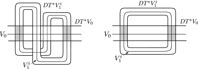
Figure 2. Plumbing description: orientable case on the left, non-orientable case on the right

Finally, there is one last vanishing cycle $V_{2}$, corresponding to the maximum of $f$, obtained by the Lagrangian surgery (see Figure 3, for an example) of $V_{0}$ with the union $\bigcup_{i=1}^{m}V^{1}_{i}$.

Figure 3. Left: Two Lagrangian curves $L_{0}$ and $L_{1}$ on a surface intersecting locally as shown. Right: Lagrangian surgery $L_{0}\#L_{1}$

By the discussion in Section 2, the $4$-manifold $E$ admits an exact symplectic form $\omega$, for which $\pi:E\to D^{2}$ is an exact symplectic Lefschetz fibration. Moreover, Johns verified that

• $S$ admits an exact Lagrangian embedding into $E$.

• The critical points of $\pi$ lie on $S$, $\pi(S)\subset\mathbb{R}$, and $\pi|_{S}=f$.

• The symplectic manifold $(E,\omega)$, after smoothing the corners of $E$, is conformally exact symplectomorphic to $(DT^{*}S,\omega_{can})$.

Apparently, the most difficult step is the first item above. In order to find such an embedding Johns used a “Milnor-type” handle decomposition—a more refined version of a usual handle decomposition—of the surface $S$, referring to [19, pages 27-32]. Once this is achieved, the second item follows from the first by construction. The last item is essentially a retraction of $E$, by a Liouville type flow, onto a small Weinstein neighborhood of $S$, which is symplectomorphic to $(DT^{*}S,\omega_{can})$.

In order to prove the main results of our article, we focus on the orientable surface case in Section 3.1, while in Section 3.2, we treat the non-orientable surface case. For both cases, we use a handle decomposition of a closed surface induced by the standard Morse function with one minimum and one maximum, although this assumption can be removed as pointed out in [13, Section 4.3].

3.1. Unit contact cotangent bundles of orientable surfaces

In this section, we assume that $S$ is a closed orientable surface of genus $g$, which we denote by $\Sigma_{g}$. We also denote the exact symplectic Lefschetz fibration of Johns described above by $\pi_{g}:(W_{g},\omega_{g})\rightarrow D^{2}$, where $(W_{g},\omega_{g})$ is conformally exact symplectomorphic to $(DT^{*}\Sigma_{g},\omega_{can})$. We first review the Lefschetz fibration $\pi_{g}$, primarily focusing on its topological aspects.

The regular fiber $F_{g}$ of $\pi_{g}$ is diffeomorphic to an oriented genus $g$ surface with $2g+2$ boundary components. In the following, we describe the construction of $F_{g}$, referring to Figure 4.

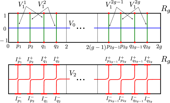
Figure 4. The vanishing cycles $V_{0},V_{1}^{1},\dots,V_{1}^{g},V_{2}$

Let $R_{g}$ denote the rectangle $[0,2g]\times[-1,1]$ in $\mathbb{R}^{2}$ equipped with the standard orientation. We fix the following points

$$p_{2i-1}:=2(i-1)+1/3,\;p_{2i}:=2(i-1)+2/3,$$

$$q_{2i-1}:=2(i-1)+4/3,\;q_{2i}:=2(i-1)+5/3,$$

for $i=1,2,\dots,g$, on the $x$-axis. For a sufficiently small $\varepsilon>0$, we set

$$I^{\pm}_{p_{j}}:=[p_{j}-\varepsilon,p_{j}+\varepsilon]\times\{\pm 1\},\ I^{\pm}_{q_{j}}:=[q_{j}-\varepsilon,q_{j}+\varepsilon]\times\{\pm 1\}\subset R_{g}$$

for $j=1,2,\dots,2g$. We identify $\{0\}\times[-1,1]\subset R_{g}$ with $\{2g\}\times[-1,1]\subset R_{g}$ to obtain an annulus initially. Next, for each $j=1,2,\ldots,2g$, we identify $I_{p_{j}}^{+}$ with $I_{q_{j}}^{-}$, and $I_{p_{j}}^{-}$ with $I_{q_{j}}^{+}$ so that the orientation of $R_{g}$ extends to the resulting surface $F_{g}$.

Note that, for each $j=1,2,\ldots,2g$, these identifications can be viewed as attaching two $1$-handles, which is the same as plumbing an annulus as shown on the left in Figure 2.

By calculating the Euler characteristic, for example, it can be easily seen that $F_{g}$ is diffeomorphic to an oriented genus $g$ surface with $2g+2$ boundary components.

By fixing a certain choice of distinguished set of vanishing paths, the $2g+2$ vanishing cycles $V_{0},V_{1}^{1},V_{1}^{2},\dots,V_{1}^{2g},V_{2}$ of the Lefschetz fibration $\pi_{g}$, are given as follows. The vanishing cycle $V_{0}$ is the simple closed curve in $F_{g}$ obtained from $[0,2g]\times\{0\}\subset R_{g}$ through the above identifications. Similarly, the simple closed curve $V_{1}^{j}\subset F_{g}$ is obtained from $(\{p_{j}\}\times[-1,1])\cup(\{q_{j}\}\times[-1,1])\subset R_{g}$. Equivalently, $V_{1}^{j}$ is the core circle of the annulus that appears in the plumbing description (see Figure 2). The vanishing cycle $V_{2}\subset F_{g}$ comes from the Lagrangian surgery of $V_{0}$ and $\cup_{i=1}^{2g}V_{1}^{j}$ as depicted at the bottom of Figure 4.

Next we show that the vanishing cycles $V_{0},V_{1}^{1},V_{1}^{2},\dots,V_{1}^{2g},V_{2}$ can be presented with a different point of view, by reconstructing $F_{g}$ as follows. Let

$$A_{i}:=[2(i-1),2i]\times[-1,1]\subset R_{g}$$

for $i=1,2,\dots,g$ and let

$$J_{j}:=\{j\}\times[-1,1]$$

for $j=0,1,\dots,2g$. It is clear that $R_{g}=\cup_{i=1}^{g}A_{i}$. Then we divide each $A_{i}$ into two pieces

$$A_{i}^{+}:=[2(i-1),2i-1]\times[-1,1],\;\ A_{i}^{-}:=[2i-1,2i]\times[-1,1]$$

and put $A_{i}^{+}$ vertically on top of $A_{i}^{-}$ as shown in Figure 5 (a).

Since $I^{\pm}_{p_{2i-1}}$ and $I^{\pm}_{p_{2i}}$ belong to $A_{i}^{+}$ and $I^{\pm}_{q_{2i-1}}$ and $I^{\pm}_{q_{2i}}$ belong to $A_{i}^{-}$, we can glue $A_{i}^{+}$ and $A_{i}^{-}$ along these intervals. Each of these gluings is represented by a $1$-handle in Figure 5 (b). Moreover, we identify $J_{2i-1}\subset A_{i}^{+}$ with $J_{2i-1}\subset A_{i}^{-}$, which is also represented by a $1$-handle. There is another $1$-handle associated to the identification of $J_{2i}\subset A_{i}^{-}$ with $J_{2i}\subset A_{i+1}^{+}$. We slide this $1$-handle over the one coming from the identification of $I_{p_{2i}}^{+}$ with $I_{q_{2i}}^{-}$ as indicated in Figure 5 (c).

Starting from the diagram in Figure 5 (c), and performing isotopies as shown in Figure 6, we now obtain a genus $1$ surface with $3$ boundary components. We call this surface the “building block”, and denote it by $F_{g}^{i}$. The key point is that the surface $F_{g}$ can be constructed by assembling these building blocks, which looks pairwise identical.

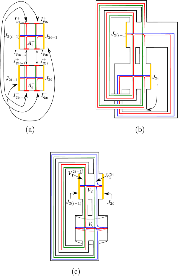
Figure 5. The building block $F_{g}^{i}$

Note that the vanishing cycles can also be isotoped through the identifications and isotopies described above. As a result, in each $F_{g}^{i}$, we see two arcs $\tilde{V}_{0}^{i}$ and $\tilde{V}_{2}^{i}$ which are subarcs of $V_{0}$ and $V_{2}$, respectively. We also see two simple closed curves $V_{1}^{2i-1}$ and $V_{1}^{2i}$, as depicted on the right in Figure 6. Finally, to describe $F_{g}$ and the vanishing cycles $V_{0},V_{1}^{1},\dots,V_{1}^{2g},V_{2}$, we arrange $F_{g}^{1},\dots,F_{g}^{g}$ in a circular position, glue $F_{g}^{i}$ to $F_{g}^{i+1}$ along $J_{2i}$ for $i=1,\dots,g-1$ and glue $F_{g}^{g}$ to $F_{g}^{1}$ along $J_{2g}$ and $J_{0}$ as shown in Figure 7.

Since the fiber $F_{g}$ is a genus $g$ surface with $2g+2$ boundary components, we opted to denote it with $\Sigma_{g,2g+2}$ in Theorem 3.1.

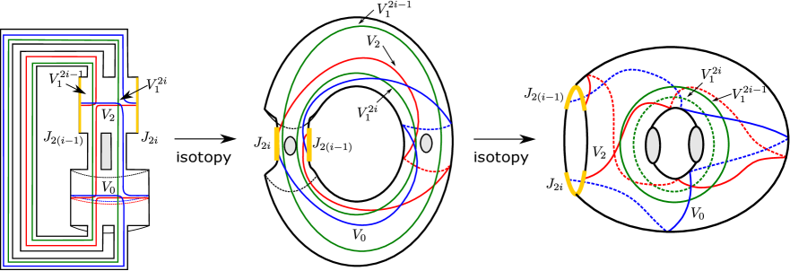
Figure 6. Isotoping the vanishing cycles on $F_{g}^{i}$

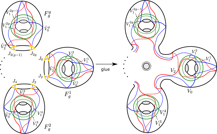
Figure 7. The vanishing cycles $V_{0},V_{1}^{1},\dots,V_{1}^{2g},V_{2}$ on the fiber $F_{g}$

Theorem 3.1.

Let $V_{0},V_{1}^{1},\dots,V_{1}^{2g},V_{2}$ be the simple closed curves shown on the surface $\Sigma_{g,2g+2}\cong F_{g}$ depicted on the right in Figure 7 and let

$$\varphi_{g}:=D(V_{0})D(V_{1}^{1})\cdots D(V_{1}^{2g})D(V_{2})\in Map(\Sigma_{g,2g+2},\partial\Sigma_{g,2g+2}).$$

Then, for all $g\geq 1$, the open book $(\Sigma_{g,2g+2},\varphi_{g})$ is adapted to $(ST^{*}\Sigma_{g},\xi_{can})$.

Proof.

We first note that the open book $(\Sigma_{g,2g+2},\varphi_{g})$ induced on $\partial W_{g}$ by

$$\pi_{g}:(W_{g},\omega_{g}=d\alpha_{g})\rightarrow D^{2}$$

is adapted to the contact $3$-manifold $(\partial W_{g},\ker(\alpha_{g}|_{\partial W_{g}}))$. According to [13, Theorem 1.1], $(W_{g},\omega_{g})$ is conformally exact symplectomorphic to $(DT^{*}\Sigma_{g},\omega_{can})$, which is a strong symplectic filling of $(ST^{*}\Sigma_{g},\xi_{can})$. As a consequence, $(\partial W_{g},\ker(\alpha_{g}|_{\partial W_{g}}))$ is contactomorphic to $(ST^{*}\Sigma_{g},\xi_{can})$, and hence $(\Sigma_{g,2g+2},\varphi_{g})$ is adapted to $(ST^{*}\Sigma_{g},\xi_{can})$. ∎

Remark 3.2.

Theorem 3.1 also holds for $g=0$ case. Note that $F_{0}=\Sigma_{0,2}$ is nothing but an annulus. In this case, $V_{0}=V_{2}$ is the core circle of this annulus, and there is no $V_{1}^{j}$. Therefore $(ST^{*}S^{2}=\mathbb{RP}^{3},\xi_{can})$ has an adapted open book whose page is an annulus and whose monodromy is the square of the positive Dehn twist along the core circle of the annulus.

3.1.1. Another open book decomposition

In this section, we describe another open book decomposition of $ST^{*}\Sigma_{g}$ supporting $\xi_{can}$. To motivate our discussion, we digress here to review some open book of $ST^{*}\Sigma_{1}\cong T^{3}$ supporting $\xi_{can}$ given by Van Horn-Morris [22]. Our goal is to compare this open book with the one described in Theorem 3.1, for the case $g=1$. The page of the open book described in [22, Chapter 6] is diffeomorphic to a $4$-holed torus $\Sigma_{1,4}$ and its monodromy is given by

$$\widetilde{\varphi}_{1}:=D^{-2}(a_{1})D^{-2}(a_{2})D^{-2}(a_{3})D^{-2}(a_{4})D(\delta_{1})D(\delta_{2})D(\delta_{3})D(\delta_{4}),$$

where $a_{1},a_{2},a_{3},a_{4},\delta_{1},\delta_{2},\delta_{3},\delta_{4}$ are shown on the $4$-holed torus $\Sigma_{1,4}$ depicted in Figure 8.

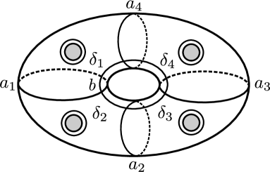
Figure 8. $4$-holed torus $\Sigma_{1,4}$

Using the relation (cf. [14])

$$D(\delta_{1})D(\delta_{2})D(\delta_{3})D(\delta_{4})=(D(a_{1})D(a_{3})D(b)D(a_{2})D(a_{4})D(b))^{2}\in Map(\Sigma_{1,4},\partial\Sigma_{1,4})$$

and setting $A_{1,3}:=D(a_{1})D(a_{3})$, $A_{2,4}:=D(a_{2})D(a_{4})$, we see that $\widetilde{\varphi}_{1}$ is equivalent to a product of four positive Dehn twists:

$$\widetilde{\varphi}_{1}=A_{2,4}^{-1}A_{1,3}^{-1}A_{2,4}^{-1}A_{1,3}^{-1}A_{1,3}D(b)A_{2,4}D(b)A_{1,3}D(b)A_{2,4}D(b)$$

$$=A_{2,4}^{-1}\big{[}A_{1,3}^{-1}\big{(}(A_{2,4}^{-1}D(b)A_{2,4})D(b)\big{)}A_{1,3}D(b)\big{]}A_{2,4}D(b)$$

$$=D(A_{2,4}^{-1}A_{1,3}^{-1}A_{2,4}^{-1}(b))\;D(A_{2,4}^{-1}A_{1,3}^{-1}(b))\;D(A_{2,4}^{-1}(b))\;D(b)$$

$$\equiv D(A_{2,4}^{-1}(b))\;D(b)\;D(A_{1,3}(b))\;D(A_{1,3}A_{2,4}(b)),$$

where the notation “$\equiv$” means “related by a global conjugation”. Here we conjugated with the diffeomorphism $A_{1,3}A_{2,4}$, to obtain the last line from the previous one. We would like to compare this open book with the one described in Theorem 3.1, for the case $g=1$. The latter has monodromy

$$\varphi_{1}=D(V_{0})D(V_{1}^{1})D(V_{1}^{2})D(V_{2})\in Map(\Sigma_{1,4},\partial\Sigma_{1,4}),$$

where the curves $V_{0},V_{1}^{1},V_{1}^{2},V_{2}$ are depicted in Figure 9.

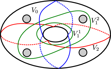
Figure 9. The vanishing cycles $V_{0},V_{1}^{1},V_{1}^{2},V_{2}$ on $\Sigma_{1,4}$

Now one can easily verify that $V_{0}=A_{2,4}^{-1}(b)$, $V_{1}^{1}=b$, $V_{1}^{2}=A_{2,4}^{-1}A_{1,3}(b)$, and $V_{2}=A_{1,3}(b)$, using our notation above.

Hence we get

$$\varphi_{1}=D(A_{2,4}^{-1}(b))\;D(b)\;D(A_{2,4}^{-1}A_{1,3}(b))\;D(A_{1,3}(b)),$$

and we claim that $\varphi_{1}$ and $\widetilde{\varphi}_{1}$ are Hurwitz-equivalent. To see this, we apply a Hurwitz move to $\widetilde{\varphi}_{1}$. Namely, we switch the order of the last two Dehn twists in the factorization of $\widetilde{\varphi}_{1}$ as follows:

$$D(A_{2,4}^{-1}(b))\;D(b)\;D(A_{1,3}D(b)A^{-1}_{1,3}A_{1,3}A_{2,4}(b))\;D(A_{1,3}(b)).$$

Here we used the relation $D(A_{1,3}(b))=A_{1,3}D(b)A^{-1}_{1,3}$. To prove our claim, one can simply verify that $A_{1,3}D(b)A^{-1}_{1,3}A_{1,3}A_{2,4}(b)$ is isotopic to $A_{2,4}^{-1}A_{1,3}(b)$ by a direct calculation on the surface $\Sigma_{1,4}$.

The upshot is that the open books (both of whose page is a $4$-holed torus) given by monodromies $\varphi_{1}$ and $\widetilde{\varphi}_{1}$, respectively, are indeed isomorphic. Moreover, there is an exact symplectic Lefschetz fibration $\widetilde{\pi}_{1}:(\widetilde{W}_{1},\widetilde{\omega}_{1})\to D^{2}$ whose monodromy is $\widetilde{\varphi}_{1}$. Recall that we already considered an exact symplectic Lefschetz fibration $\pi_{1}:(W_{1},\omega_{1})\rightarrow D^{2}$ whose monodromy is $\varphi_{1}$, at the beginning of Section 3. By Lemma 2.6, we immediately deduce the following corollary.

Corollary 3.3.

The exact symplectic Lefschetz fibrations $\pi_{1}:(W_{1},\omega_{1})\rightarrow D^{2}$ and $\widetilde{\pi}_{1}:(\widetilde{W}_{1},\widetilde{\omega}_{1})\to D^{2}$ are isomorphic through an exact symplectomorphism.

In his thesis [22, Chapter 4], Van Horn-Morris describes another open book adapted to the contact $3$-manifold $(ST^{*}\Sigma_{1},\xi_{can})$, whose page is a $3$-holed torus $\Sigma_{1,3}$ (rather than $4$-holed) and whose monodromy is given by

$$\psi_{1}=D(\delta_{1})D(\delta_{2})D(\delta_{3})D^{-3}(a_{1})D^{-3}(a_{2})D^{-3}(a_{3}),$$

where $a_{1},a_{2},a_{3},b,\delta_{1},\delta_{2},\delta_{3}$ are shown on the $3$-holed torus $\Sigma_{1,3}$ depicted in Figure 10.

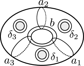
Figure 10. $3$-holed torus $\Sigma_{1,3}$

By using the star relation $D(\delta_{1})D(\delta_{2})D(\delta_{3})=(D(b)D(a_{1})D(a_{2})D(a_{3}))^{3}$, and setting

$$T=D(a_{1})D(a_{2})D(a_{3}),$$

we have

$$\psi_{1}=D(\delta_{1})D(\delta_{2})D(\delta_{3})D^{-3}(a_{1})D^{-3}(a_{2})D^{-3}(a_{3})$$

$$=(D(b)T)^{3}T^{-3}$$

$$=D(b)TD(b)TD(b)T^{-2}$$

$$\equiv(T^{-1}D(b)T)D(b)(TD(b)T^{-1})$$

$$=D(T^{-1}(b))\;D(b)\;D(T(b)).$$

Hence we see that the monodromy of this open book is equivalent to the product of three positive Dehn twists. Moreover, since both $(\Sigma_{1,3},\psi_{1})$ and $(\Sigma_{1,4},\widetilde{\varphi}_{1})$, are adapted to the contact $3$-manifold $(ST^{*}\Sigma_{1},\xi_{can})$, they must have a common positive stabilization. As a matter of fact, one can easily verify that $(\Sigma_{1,3},\psi_{1})$ stabilized twice and $(\Sigma_{1,4},\widetilde{\varphi}_{1})$ stabilized once are equivalent, using the lantern relation.

Motivated by the genus one case, for each $g\geq 1$, we construct an open book adapted to $(ST^{*}\Sigma_{g},\xi_{can})$ whose page is diffeomorphic to $\Sigma_{g,g+2}$, reducing the number of boundary components of the page, compared to that which appeared in Theorem 3.1. The key idea is to cut down one boundary component for each building block that we used above to construct the page $F_{g}$. To construct this new open book adapted to $(ST^{*}\Sigma_{g},\xi_{can})$, we introduce a new building block, inspired by the genus one case. We set $u_{0}:=T^{-1}(b)$ and $\ u_{2}:=T(b)$, as depicted in Figure 11.

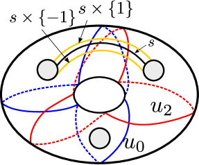
Figure 11. The curves $u_{0}$, $u_{2}$ and the arc $s$ on $\Sigma_{1,3}$

Let $s$ be the arc whose endpoints lie on two distinct boundary components in a $3$-holed torus $\Sigma_{1,3}$ as shown in Figure 11 and let $N(s)$ denote a tubular neighborhood of $s$. We write $\tilde{\Sigma}$ for the resulting surface, after removing $s\times(-1,1)$ from $\Sigma_{1,3}$, where we identify $N(s)$ with $s\times[-1,1]$. We write $\tilde{u}_{0}$ and $\tilde{u}_{2}$ for the two arcs in $\tilde{\Sigma}$ obtained from the curves $u_{0}$ and $u_{2}$, respectively, by removing their intersection with $N(s)$.

We take $g$ copies of $\tilde{\Sigma}$ and denote each copy by $\tilde{\Sigma}_{j}$, for $j=1,\ldots,g$. We set

$$s_{j}\times\{\pm 1\}:=s\times\{\pm 1\}\subset\tilde{\Sigma}_{j},$$

$$\tilde{u}_{i}^{j}:=\tilde{u}_{i}\subset\tilde{\Sigma}_{j}{(i=0,2)},\;\tilde{u}_{1}^{j}:=u_{1}\subset\tilde{\Sigma}_{j},$$

and put $\tilde{\Sigma}_{1},\tilde{\Sigma}_{2},\dots,\tilde{\Sigma}_{g}$ in a circular position as depicted on the left in Figure 12. Now, we glue $\tilde{\Sigma}_{j}$ to $\tilde{\Sigma}_{j+1}$ by identifying $s_{j}\times\{1\}$ with $s_{j+1}\times\{-1\}$ for $j=1,2,\dots,g-1$ and we glue $\tilde{\Sigma}_{g}$ to $\tilde{\Sigma}_{1}$ by identifying $s_{g}\times\{1\}$ with $s_{1}\times\{-1\}$. As a consequence, we obtain a surface diffeomorphic to $\Sigma_{g,g+2}$, which is depicted on the right in Figure 12. Via the identifications above, the union of the arcs $\tilde{u}_{0}^{j}$ and $\tilde{u}_{2}^{j}$ form simple closed curves $U_{0}$ and $U_{2}$, respectively, in $\Sigma_{g,g+2}$. Considering $\tilde{\Sigma}_{j}$ as a subsurface of $\Sigma_{g,g+2}$, we denote $u_{1}^{j}$ by $U_{1}^{j}$.

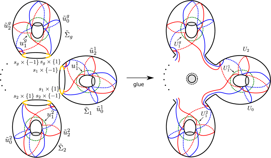
Figure 12. The curves $U_{0},U_{1}^{1},\ldots,U_{1}^{g},U_{2}$ on the page $\Sigma_{g,g+2}$

Theorem 3.4.

Let $U_{0},U_{1}^{1},\ldots,U_{1}^{g},U_{2}$ be the simple closed curves shown on $\Sigma_{g,g+2}$ depicted on the right in Figure 12 and let

$$\psi_{g}:=D(U_{0})D(U_{1}^{1})\cdots D(U_{1}^{g})D(U_{2})\in Map(\Sigma_{g,g+2},\partial\Sigma_{g,g+2}).$$

Then, for all $g\geq 1$, the open book $(\Sigma_{g,g+2},\psi_{g})$ is adapted to $(ST^{*}\Sigma_{g},\xi_{can})$.

Proof.

We show that $(\Sigma_{g,g+2},\psi_{g})$ and $(\Sigma_{g,2g+2},\varphi_{g})$ have a common positive stabilization. The result follows from a theorem of Giroux [10] coupled with our Theorem 3.1. Let $\alpha_{1,j},\alpha_{2,j},\dots,\alpha_{5,j},\beta_{j}$ (for $j=1,2,\dots,g$), and $\gamma$ be the simple closed curves on $\Sigma_{g,4g+2}$ as shown in Figure 13.

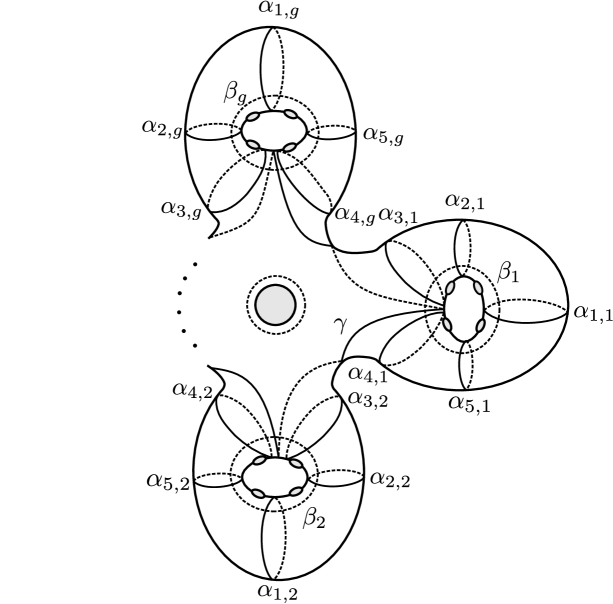
Figure 13. We illustrate a genus $g$ surface $\Sigma_{g,4g+2}$ with $4g+2$ boundary components. There are two boundary components at the center: one is on top indicated by the solid circle whose interior is shaded; the other one is on the back side of the surface indicated by the dashed circle.

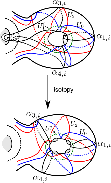
Figure 14. Each “building block” in the open book $(\Sigma_{g,g+2},\psi_{g})$ is stabilized three times, where the stabilizing curves $\alpha_{1,i},\alpha_{3,i}$ and $\alpha_{4,i}$ are pairwise disjoint. To go from top to bottom, we just move the newly created two holes (on the top-left) by an isotopy, along with the curves $\alpha_{3,i}$ and $\alpha_{4,i}$.

In order to prove our claim, we first stabilize the open book $(\Sigma_{g,g+2},\psi_{g})$ $3g$ times as indicated in Figure 14. Here we just illustrate three stabilizations on each building block, where the stabilizing curves are $\alpha_{1,i},\alpha_{3,i}$ and $\alpha_{4,i}$. The page of the resulting open book is $\Sigma_{g,4g+2}$ (identified with the surface in Figure 13) and the monodromy $\widehat{\psi_{g}}\in Map(\Sigma_{g,4g+2},\partial\Sigma_{g,4g+2})$ is given by

$\widehat{\psi_{g}}=\psi_{g}D(\alpha_{1,1})\cdots D(\alpha_{1,g})D(\alpha_{3,1})\cdots D(\alpha_{3,g})D(\alpha_{4,1})\cdots D(\alpha_{4,g})$,

where $\psi_{g}$ is extended to $\Sigma_{g,4g+2}$ by identity.

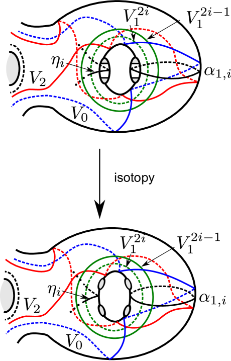
Figure 15. Each “building block” in the open book $(\Sigma_{g,2g+2},\varphi_{g})$ is stabilized twice, where the stabilizing curves $\eta_{i}:=D^{-1}(V_{2})D^{-1}(\beta_{i})(\alpha_{4,i})$ and $\alpha_{1,i}$ are disjoint.

Similarly, we stabilize the open book $(\Sigma_{g,2g+2},\varphi_{g})$ $2g$ times as indicated in Figure 15. Here we just illustrate two stabilizations on each building block, where the stabilizing curves are $\alpha_{1,i}$ and $\eta_{i}:=D^{-1}(V_{2})D^{-1}(\beta_{i})(\alpha_{4,i})$. The page of the resulting open book is $\Sigma_{g,4g+2}$ (identified with the surface in Figure 13) and the monodromy $\widehat{\varphi_{g}}\in Map(\Sigma_{g,4g+2},\partial\Sigma_{g,4g+2})$ is given by

$\widehat{\varphi}_{g}=\varphi_{g}D(\eta_{1})\cdots D(\eta_{g})D(\alpha_{1,1})\cdots D(\alpha_{1,g})$,

where $\varphi_{g}$ is extended to $\Sigma_{g,4g+2}$ by identity.

Now we claim that $\widehat{\psi}_{g}$ and $\widehat{\varphi}_{g}$ are conjugate. First of all, both $\widehat{\psi}_{g}$ and $\widehat{\varphi}_{g}$ can be viewed as self-diffeomorphisms of the surface $\Sigma_{g,4g+2}$ shown in Figure 13. In the following, we express the curves involved in the definitions of $\widehat{\psi}_{g}$ and $\widehat{\varphi}_{g}$ in terms of those depicted in Figure 13. For convenience, we set

$\alpha_{i}:=\cup_{j=1}^{g}\alpha_{i,j},\;\;\;\;\beta:=\cup_{j=1}^{g}\beta_{j},\;\;\;\;D(\alpha_{i}):=\Pi_{j=1}^{g}D(\alpha_{i,j}),\;\;\;\;D(\beta):=\Pi_{j=1}^{g}D(\beta_{j}).$

Then, we have

$U_{0}=D^{-1}(\alpha_{2})D^{-1}(\alpha_{5})D(\beta)(\gamma),\;\;\;\;\;U_{1}^{j}=\beta_{j},\;\;\;\;\;U_{2}=D(\alpha_{2})D(\alpha_{5})D^{-1}(\beta)(\gamma),$

$V_{0}=D(\alpha_{4})D^{-1}(\alpha_{2})D^{-1}(\alpha_{5})D(\beta)(\gamma)=D(\alpha_{4})(U_{0}),\;\;\;\;\;V_{1}^{2j-1}=D^{-1}(\alpha_{3,j})D(\alpha_{4,j})(\beta_{j})$,

$V_{1}^{2j}=\beta_{j},\;\;\;\;\;V_{2}=D^{-1}(\alpha_{3})D(\alpha_{2})D(\alpha_{5})D^{-1}(\beta)(\gamma)=D^{-1}(\alpha_{3})(U_{2})$.

In the following argument, we write $D(\alpha_{i})D(\beta)D^{-1}(\alpha_{i})$ for $\Pi_{j=1}^{g}(D(\alpha_{i,j})D(\beta_{j})D^{-1}(\alpha_{i,j}))$, and this is justified by the fact that $D(\alpha_{i,k})D(\beta_{j})=D(\beta_{j})D(\alpha_{i,k})$ for $k\neq j$.

Using the notation “$\equiv$” for “related by a cyclic permutation or a Hurwitz move”, and underlining each pair of Dehn twists where we perform a Hurwitz move, we have

$$\widehat{\psi}_{g}=\psi_{g}D(\alpha_{1,1})\cdots D(\alpha_{1,g})D(\alpha_{3,1})\cdots D(\alpha_{3,g})D(\alpha_{4,1})\cdots D(\alpha_{4,g})$$

$$=D(U_{0})D(U_{1}^{1})\cdots D(U_{1}^{g})D(U_{2})\underline{D(\alpha_{1})D(\alpha_{3})}{D(\alpha_{4})}$$

$$\equiv D(D^{-1}(\alpha_{2})D(\alpha_{5})D(\beta)(\gamma))D(\beta)D(D(\alpha_{2})D(\alpha_{5})D^{-1}(\beta)(\gamma))D(\alpha_{3})D(\alpha_{1}){D(\alpha_{4})}$$

$$\equiv\underline{D(\alpha_{4})D(D^{-1}(\alpha_{2})D(\alpha_{5})D(\beta)(\gamma))}D(\beta)\underline{D(D^{-1}(\alpha_{2})D(\alpha_{5})D^{-1}(\beta)(\gamma))D(\alpha_{3})}D(\alpha_{1})$$

$$\equiv D(D(\alpha_{4})D^{-1}(\alpha_{2})D(\alpha_{5})D(\beta)(\gamma))D(\alpha_{4})D(\beta)D(\alpha_{3})D(D^{-1}(\alpha_{3})D(\alpha_{2})D(\alpha_{5})D^{-1}(\beta)(\gamma))D(\alpha_{1})$$

$$=D(V_{0})\underline{D(\alpha_{4})D(\beta)}D(\alpha_{3})D(V_{2})D(\alpha_{1})$$

$$\equiv D(V_{0})D(D(\alpha_{4})(\beta))\underline{D(\alpha_{4})D(\alpha_{3})}D(V_{2})D(\alpha_{1})$$

$$\equiv D(V_{0})\underline{D(D(\alpha_{4})(\beta))D(\alpha_{3})}D(\alpha_{4})D(V_{2})D(\alpha_{1})$$

$$\equiv D(V_{0})D(\alpha_{3})D(D^{-1}(\alpha_{3})D(\alpha_{4})(\beta))D(\alpha_{4})D(V_{2})D(\alpha_{1})$$

$$\equiv D(V_{0})\underline{D(\alpha_{3})\{\Pi_{j=1}^{g}D(V_{1}^{2j-1})\}}D(\alpha_{4})D(V_{2})D(\alpha_{1})$$

$$\equiv D(V_{0})\{\Pi_{j=1}^{g}D(V_{1}^{2j-1})\}D(\{\Pi_{j=1}^{g}D^{-1}(V_{1}^{2j-1})\}(\alpha_{3}))D(\alpha_{4})D(V_{2})D(\alpha_{1})$$

Using the fact that $D^{-1}(V_{1}^{2j-1})(\alpha_{3,j})$ and $D(\alpha_{4,j})(\beta_{j})$ are isotopic, we continue the sequence of equivalences above as

$$=D(V_{0})\{\Pi_{j=1}^{g}D(V_{1}^{2j-1})\}\underline{D(D(\alpha_{4})(\beta))D(\alpha_{4})}D(V_{2})D(\alpha_{1})$$

$$\equiv D(V_{0})\{\Pi_{j=1}^{g}D(V_{1}^{2j-1})\}\underline{D(\alpha_{4})D(\beta)}D(V_{2})D(\alpha_{1})$$

$$\equiv D(V_{0})\{\Pi_{j=1}^{g}D(V_{1}^{2j-1})\}D(\beta)\underline{D(D^{-1}(\beta)(\alpha_{4}))D(V_{2})}D(\alpha_{1})$$

$$\equiv D(V_{0})\{\Pi_{j=1}^{g}D(V_{1}^{2j-1})\}\{\Pi_{j=1}^{g}D(V_{1}^{2j})\}D(V_{2})D(D^{-1}(V_{2})D^{-1}(\beta)(\alpha_{4}))D(\alpha_{1})$$

$$\equiv D(V_{0})\{\Pi_{j=1}^{g}D(V_{1}^{2j-1})\}\{\Pi_{j=1}^{g}D(V_{1}^{2j})\}D(V_{2})\{\Pi_{j=1}^{g}D(\eta_{j})\}D(\alpha_{1})$$

$$=D(V_{0})\{\Pi_{j=1}^{g}D(V_{1}^{2j-1})\}\{\Pi_{j=1}^{g}D(V_{1}^{2j})\}D(V_{2})\{\Pi_{j=1}^{g}D(\eta_{j})\}D(\alpha_{1})$$

$$=\varphi_{g}D(\eta_{1})\cdots D(\eta_{g})D(\alpha_{1,1})\cdots D(\alpha_{1,g})$$

$$=\widehat{\varphi}_{g}.$$

Since a cyclic permutation is equivalent to a global conjugation of the monodromy, and a Hurwitz move does not affect the monodromy, we conclude that $\widehat{\psi}_{g}=\widehat{\varphi}_{g}$ up to conjugation. Therefore, the open books $(\Sigma_{g,g+2},{\psi}_{g})$ and $(\Sigma_{g,2g+2},{\varphi_{g}})$ have a common positive stabilization.∎

Corollary 3.5.

Let $\pi_{g}^{\prime}:(W_{g}^{\prime},\omega_{g}^{\prime})\rightarrow D^{2}$ denote the exact symplectic Lefschetz fibration, whose regular fiber is $\Sigma_{g,g+2}$ and whose monodromy is

$$\psi_{g}=D(U_{0})D(U_{1}^{1})\cdots D(U_{1}^{g})D(U_{2}).$$

Then, for all $g\geq 1$, the completion of $(W_{g}^{\prime},\omega_{g}^{\prime})$ is symplectomorphic to the completion of $(DT^{*}\Sigma_{g},\omega_{can})$. In particular, $W_{g}^{\prime}$ is diffeomorphic to $DT^{*}\Sigma_{g}$.

Proof.

By the proof of Theorem 3.4, we see that $\pi_{g}$ (defined at the beginning of Section 3) and $\pi_{g}^{\prime}$ have a common positive stabilization, up to Hurwitz moves and global conjugations. Note that a global conjugation induces an isomorphism of exact symplectic Lefschetz fibrations through a symplectomorphism of their total spaces. Therefore, the statement follows by combining Lemma 2.6 and Lemma 2.7.∎

As mentioned in Section 1, according to Wendl [24], any minimal strong symplectic filling of $(ST^{*}\Sigma_{1}\cong T^{3},\xi_{can})$ is symplectic deformation equivalent to $(DT^{*}\Sigma_{1}\cong T^{2}\times D^{2},\omega_{can})$. Therefore, we would like to finish this section with the following question.

Question 3.6.

Is it true that $(W_{g}^{\prime},\omega_{g}^{\prime})$ in Corollary 3.5 is symplectic deformation equivalent to $(DT^{*}\Sigma_{g},\omega_{can})$, for all $g\geq 2$?

It is plausible that the answer to Question 3.6 is positive, via a Liouville type flow as in [13], although we could not verify it.

3.2. Unit contact cotangent bundles of non-orientable surfaces

In this section, we assume that $S$ is the closed non-orientable surface obtained by the connected sum of $k$ copies of $\mathbb{RP}^{2}$, which we denote by $N_{k}$. We also denote the exact symplectic Lefschetz fibration of Johns discussed above by $\pi_{k}:(M_{k},\omega_{k})\rightarrow D^{2}$, where $(M_{k},\omega_{k})$ is conformally exact symplectomorphic to $(DT^{*}N_{k},\omega_{can})$. We first review the Lefschetz fibration $\pi_{k}$ by describing its fiber and a set of vanishing cycles.

The fiber $F_{k}$ (see Figure 16) is constructed as follows: Let $R_{k}$ denote the rectangle $[0,k]\times[-1,1]$ in $\mathbb{R}^{2}$ equipped with the standard orientation.

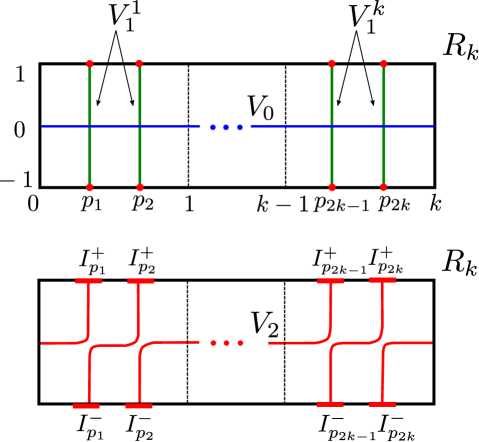
Figure 16. The vanishing cycles $V_{0},V_{1}^{1},\dots,V_{1}^{k},V_{2}$

We fix the points

$$p_{2i-1}:=(i-1)+1/3,\ p_{2i}:=(i-1)+2/3,$$

for $i=1,2,\dots,k$ on the $x$-axis. For a sufficiently small $\varepsilon>0$, set

$$I_{p_{j}}^{\pm}:=[p_{j}-\varepsilon,p_{j}+\varepsilon]\times\{\pm 1\}\subset\mathbb{R}^{2},$$

for $j=1,2,\dots,2k$. We first identify $\{0\}\times[-1,1]$ with $\{k\}\times[-1,1]$ to obtain an annulus. Next, we identify $I_{p_{2j-1}}^{+}$ with $I_{p_{2j}}^{+}$, and $I_{p_{2j-1}}^{-}$ with $I_{p_{2j}}^{-}$ for $j=1,2,\dots,k$

Note that, for each $j=1,2,\ldots,k$, these identifications can be viewed as attaching two $1$-handles, which is the same as plumbing an annulus as shown on the right in Figure 2.

It is clear (see Figure 17) that the resulting oriented surface is a planar surface with $2k+2$ boundary components.

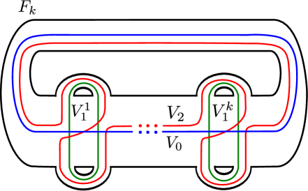
Figure 17. The vanishing cycles $V_{0},V_{1}^{1},\dots,V_{1}^{k},V_{2}$ on the fiber $F_{k}$

Now we describe the vanishing cycles $V_{0},V_{1}^{1},\dots,V_{1}^{k},V_{2}$ of $\pi_{k}$ for a fixed distinguished basis of vanishing paths. The vanishing cycle $V_{0}$ is the simple closed curve in $F_{k}$ obtained from $[0,k]\times\{0\}\subset R_{k}$ through the above identifications. Similarly, the simple closed curve $V_{1}^{j}\subset F_{k}$ is obtained from $\{p_{2j-1}\}\times[-1,1]\cup\{p_{2j}\}\times[-1,1]\subset R_{k}$. Equivalently, $V_{1}^{j}$ is the core circle of the annulus that appears in the plumbing description (see Figure 17). The last vanishing cycle $V_{2}$ is the simple closed curve in $F_{k}$ obtained from the Lagrangian surgery of $V_{0}$ and $\cup_{i=1}^{k}V_{1}^{k}$.

The following theorem is proved by the same argument we used to prove Theorem 3.1.

Theorem 3.7.

Let $V_{0},V_{1}^{1},\dots,V_{1}^{k},V_{2}$ be the simple closed curves shown on the surface $\Sigma_{0,2k+2}\cong F_{k}$ depicted in Figure 17 and let

$$\phi_{k}:=D(V_{0})D(V_{1}^{1})\cdots D(V_{1}^{k})D(V_{2})\in Map(\Sigma_{0,2k+2},\partial\Sigma_{0,2k+2}).$$

Then, for all $k\geq 1$, the open book $(\Sigma_{0,2k+2},\phi_{k})$ is adapted to $(ST^{*}N_{k},\xi_{can})$.

Remark 3.8.

Note that $F_{1}=\Sigma_{0,4}$ is the $4$-holed sphere and the monodromy

$$\phi_{1}=D(V_{0})D(V_{1}^{1})D(V_{2})$$

of the open book given in Theorem 3.7 on $ST^{*}\mathbb{RP}^{2}=L(4,1)$ is equal, by the lantern relation, to the product of positive Dehn twists along four curves each of which is parallel to a boundary component of $\Sigma_{0,4}$.

Appendix: Diffeomorphism types of the total spaces of the Lefschetz fibrations

In this appendix, we verify that the total spaces of the Lefschetz fibrations $\pi_{g}:W_{g}\to D^{2}$ (see Section 3.1) and $\pi_{k}:M_{k}\to D^{2}$ (see Section 3.2) are diffeomorphic to $DT^{*}\Sigma_{g}$ and $DT^{*}N_{k}$, respectively.

3.3. Orientable case

We show that, for each $g\geq 1$, the $4$-manifold $W_{g}$ is diffeomorphic to $DT^{*}\Sigma_{g}$ using Kirby calculus. There is a handle decomposition of the fiber $F_{g}$, after isotopy, as shown in Figure 18.

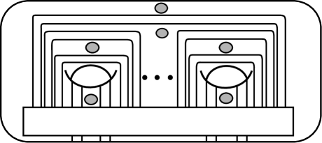
Figure 18. Handle decomposition of $F_{g}$: The large rectangle represents the $0$-handle and each band represents a $1$-handles.

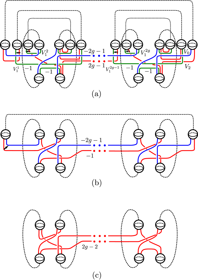
Figure 19. Kirby diagram of $W_{g}$ and Kirby calculus: Each small arrow in the diagram indicates how we slide a $2$-handle over another one.

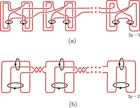
Figure 20. Kirby diagram of $W_{g}$.

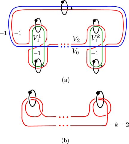
Figure 21. Kirby diagram of $M_{k}$ and the Kirby calculus.

Based on this handle decomposition of $F_{g}$ and the collection of vanishing cycles $V_{0},V_{1}^{1}$, $\dots$, $V_{1}^{2g},V_{2}$, we draw the Kirby diagram of $W_{g}$ as depicted in Figure 19 (a). Using $2$-handle slides and $1$-/$2$-handle cancelations as indicated in Figure 19 (b), we obtain the Kirby diagram shown in Figure 19 (c). Next we switch to dotted circle notation for $1$-handles, and after isotopies, we see that the Kirby diagram in Figure 20 (b) represents the disk bundle over $\Sigma_{g}$ with Euler number $2g-2$, which is indeed diffeomorphic to $DT^{*}\Sigma_{g}$.

3.4. Non-orientable case

We show that, for each $k\geq 1$, the $4$-manifold $M_{k}$ is diffeomorphic to $DT^{*}N_{k}$, again using Kirby calculus. We start with the canonical handle decomposition of the fiber $F_{k}$ (see Figure 17) and draw the Kirby diagram of $M_{k}$ as depicted in Figure 21 (a). After sliding $2$-handles and cancelling $1$-/$2$-handle pairs, we obtain the Kirby diagram shown in Figure 21 (b). This diagram shows that $M_{k}$ is diffeomorphic to a disk bundle over $N_{k}$. The Euler number of this disk bundle is $k-2$ since the framing of the $2$-handle in the diagram is $-k-2$ (cf. [11, Section 4.6]). Therefore, we conclude that $M_{k}$ is diffeomorphic to $DT^{*}N_{k}$.

Acknowledgement: We would like to thank Paul Seidel for helpful correspondence. The first author would like to express his gratitude to Koç University for its hospitality during a visit while this work was mainly carried out.

References

- [1] N. A’Campo, Real deformations and complex topology of plane curve singularities. Ann. Fac. Sci. Toulouse Math. (6) 8 (1999), no. 1, 5-23.
- [2] D. Auroux and I . Smith, Lefschetz pencils, branched covers and symplectic invariants. Symplectic 4-manifolds and algebraic surfaces. 1-53, Lecture Notes in Math., 1938, Springer, Berlin, 2008.
- [3] K. Cieliebak and Y. Eliashberg, From Stein to Weinstein and back. Symplectic geometry of affine complex manifolds. American Mathematical Society Colloquium Publications, 59. American Mathematical Society, Providence, RI, 2012.
- [4] P. Dehornoy, Genus-one Birkhoff sections for geodesic flows. Ergodic Theory Dynam. Systems 35 (2015), no. 6, 1795-1813.
- [5] Y. Eliashberg, Unique holomorphically fillable contact structure on the -torus. Internat. Math. Res. Notices 1996, no. 2, 77-82.
- [6] Y. Eliashberg, Symplectic geometry of plurisubharmonic functions. With notes by Miguel Abreu. NATO Adv. Sci. Inst. Ser. C Math. Phys. Sci., 488, Gauge theory and symplectic geometry (Montreal, PQ, 1995), 4967, Kluwer Acad. Publ., Dordrecht, 1997.
- [7] J. B. Etnyre, Planar open book decompositions and contact structures. Int. Math. Res. Not. 2004, no. 79, 4255–4267.
- [8] J. B. Etnyre and B. Ozbagci, Invariants of contact structures from open books. Trans. Amer. Math. Soc. 360 (2008), no. 6, 3133-3151.
- [9] E. Ghys, Right-handed vector fields & the Lorenz attractor. Jpn. J. Math. 4 (2009), no. 1, 47-61.
- [10] E. Giroux, Géométrie de contact: de la dimension trois vers les dimensions supérieures. (French) [Contact geometry: from dimension three to higher dimensions] Proceedings of the International Congress of Mathematicians, Vol. II (Beijing, 2002), 405-414, Higher Ed. Press, Beijing, 2002.
- [11] R. E. Gompf and A. I. Stipsicz, -manifolds and Kirby calculus. Graduate Studies in Mathematics, 20. American Mathematical Society, Providence, RI, 1999.
- [12] K. Honda, On the classification of tight contact structures, I. Geom. Topol. 4 (2000), 309-368.
- [13] J. Johns, Lefschetz fibrations on cotangent bundles of two-manifolds. Proceedings of the Gökova Geometry-Topology Conference 2011, 53-84, Int. Press, Somerville, MA, 2012.
- [14] M. Korkmaz and B. Ozbagci, On sections of elliptic fibrations. Michigan Math. J. 56 (2008), 77-87.
- [15] P. Massot, Topological methods in 3-dimensional contact geometry. Contact and symplectic topology, 27-83, Bolyai Soc. Math. Stud., 26, János Bolyai Math. Soc., Budapest, 2014.
- [16] P. Massot, Two remarks on the support genus question. http://www.math.polytechnique.fr/perso/massot.patrick/exposition/genus.pdf
- [17] D. McDuff, The structure of rational and ruled symplectic -manifolds. J. Amer. Math. Soc. 3 (1990), no. 3, 679-712.
- [18] M. McLean, Symplectic homology of Lefschetz fibrations and Floer homology of the monodromy map. Selecta Math. (N.S.) 18 (2012), no. 3, 473-512.
- [19] J. Milnor, Lectures on the h-cobordism theorem. Notes by L. Siebenmann and J. Sondow. Princeton University Press, Princeton, N.J. 1965.
- [20] B. Ozbagci and A. I. Stipsicz, Surgery on contact 3-manifolds and Stein surfaces. Bolyai Soc. Math. Stud., Vol. 13, Springer, 2004.
- [21] P. Seidel, Fukaya categories and Picard-Lefschetz theory. Zurich Lectures in Advanced Mathematics. European Mathematical Society (EMS), Zürich, 2008.
- [22] J. Van Horn-Morris, Constructions of open book decompositions. Ph.D Dissertation, UT Austin, 2007.
- [23] O. Van Koert, Lecture notes on stabilization of contact open books. arXiv:1012.4359
- [24] C. Wendl, Strongly fillable contact manifolds and J -holomorphic foliations. Duke Math. J. 151 (2010), no. 3, 337-384.