A Repelling-Attracting Metropolis Algorithm for Multimodality

Abstract

Although the Metropolis algorithm is simple to implement, it often has difficulties exploring multimodal distributions. We propose the repelling-attracting Metropolis (RAM) algorithm that maintains the simple-to-implement nature of the Metropolis algorithm, but is more likely to jump between modes. The RAM algorithm is a Metropolis-Hastings algorithm with a proposal that consists of a downhill move in density that aims to make local modes repelling, followed by an uphill move in density that aims to make local modes attracting. The downhill move is achieved via a reciprocal Metropolis ratio so that the algorithm prefers downward movement. The uphill move does the opposite using the standard Metropolis ratio which prefers upward movement. This down-up movement in density increases the probability of a proposed move to a different mode. Because the acceptance probability of the proposal involves a ratio of intractable integrals, we introduce an auxiliary variable which creates a term in the acceptance probability that cancels with the intractable ratio. Using several examples, we demonstrate the potential for the RAM algorithm to explore a multimodal distribution more efficiently than a Metropolis algorithm and with less tuning than is commonly required by tempering-based methods.

Keywords: Auxiliary variable, equi-energy sampler, forced Metropolis transition, Markov chain Monte Carlo, parallel tempering, tempered transitions.

1 Introduction and overview

Multimodal distributions are common in statistical applications. However, the Metropolis algorithm (Metropolis et al.,, 1953), one of the most widely used Markov chain Monte Carlo (MCMC) methods, tends to produce Markov chains that do not readily jump between local modes. A popular MCMC strategy for dealing with multimodality is tempering such as parallel tempering (Geyer,, 1991), simulated tempering (Geyer and Thompson,, 1995), tempered transitions (Neal,, 1996), and equi-energy sampler (Kou et al.,, 2006). Though powerful, these methods typically require extensive tuning.

Building on Metropolis, we construct an alternative multimodal sampler called the repelling-attracting Metropolis (RAM) algorithm, which is essentially as easy to implement as the original Metropolis algorithm. RAM encourages a Markov chain to jump between modes more frequently than Metropolis, and with less tuning requirements than tempering methods. Since RAM is more likely to jump between modes than Metropolis, the proportions of its iterations that are associated with each mode are more reliable estimates of their relative masses.

RAM generates a proposal via forced downhill and forced uphill Metropolis transitions. The term forced emphasizes that neither Metropolis transition is allowed to stay at its current state because we repeatedly make proposals until one is accepted. The forced downhill Metropolis transition uses a reciprocal ratio of the target densities in its acceptance probability. This encourages the intermediate proposal to prefer downward moves since a lower density state has a higher chance of being accepted, hence local modes become repelling. The subsequent forced uphill Metropolis transition generates a final proposal with a standard Metropolis ratio that makes local modes attracting. Together the downhill and uphill transitions form a proposal for a Metropolis-Hastings (MH) sampler (Hastings,, 1970), as shown in Fig. 1; a final accept-reject step preserves the stationary distribution.

As with other MH samplers, the normalizing constant of the target density need not be known, but the scale of the (symmetric) jumping rules used within the downhill and uphill transitions needs to be tuned. In principle, RAM is designed to improve Metropolis’ ability to jump between modes using the same jumping rule as Metropolis where this jumping rule is tuned to optimize the underlying Metropolis sampler for the multimodal target. One could do still better with additional tuning of RAM, but in our experience even with no additional tuning, RAM can perform better than its underlying Metropolis sampler.

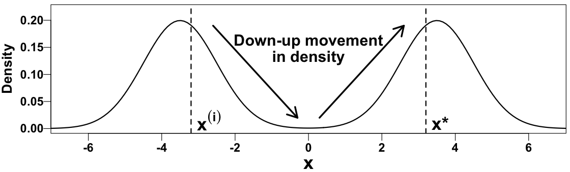
Figure 1: A repelling-attracting Metropolis algorithm is a Metropolis-Hastings algorithm that generates a proposal $x^{\ast}$ given the current state $x^{(i)}$ by making a down-up movement in density, i.e., repelling-attracting to local modes, via forced downhill and uphill Metropolis transitions. The proposal $x^{\ast}$ has a higher chance to be near a mode other than the one of the current state, and it is then accepted or rejected in the usual way to preserve the stationary distribution.

Although we can draw a sample using the down-up jumping rule, the overall acceptance probability contains a ratio of intractable integrals. We can avoid evaluating this ratio by introducing an auxiliary variable (Møller et al.,, 2006). This preserves the target marginal distribution and requires another forced downhill Metropolis transition for the auxiliary variable. Thus, RAM generates a proposal via three forced Metropolis transitions but accepts the proposal with an easy-to-compute acceptance probability.

RAM is related to a number of existing algorithms. The down-up proposal of RAM may be viewed as a simpler version of a mode-jumping proposal (Tjelmeland and Hegstad,, 2001) whose uphill movement is achieved by a deterministic optimizer. Also, the forced Metropolis transition of RAM is similar to the delayed rejection method (Tierney and Mira,, 1999; Trias et al.,, 2009) in that both generate proposals repeatedly until one is accepted. RAM’s forced transition is a special case of the delayed rejection method in that RAM uses the same jumping rule throughout while delayed rejection allows different jumping rules.

In a series of four numerical examples, we compare RAM’s performance to Metropolis and commonly used tempering-based methods such as the equi-energy sampler, parallel tempering, and tempered transitions. We adjust for the required number of evaluations of the target density or the overall CPU time required by each sampler. Our examples range from relatively simple and high dimensional Gaussian mixtures (Examples 1 and 2) to lower dimensional, but more complex targets that arise as posterior distributions in scientific problems (Examples 3 and 4). We compare RAM with standard Metropolis, implementing both samplers with a common jumping rule that is tuned to improve the mixing of Metropolis for the particular multimodal target distribution. These comparisons suggest that replacing Metropolis with RAM when targeting a multimodal distribution can be an efficient strategy, in terms of user’s effort.

In our comparisons with tempering-based samplers, we find that in moderate dimensions RAM performs as well as or better than tempering-based methods, without the subtle tuning that these methods require. Even with a higher dimensional target distribution in Example 3, we show how RAM can be embedded within a Gibbs sampler to obtain results as good as tempering-based methods, again without the tuning they require. Because RAM is able to jump between modes relatively often, it provides good estimates of the relative size of the modes. In our examples RAM obtains more reliable estimates of the mode sizes than Metropolis and is easier to directly implement than tempering-based methods.

2 A repelling-attracting Metropolis algorithm

2.1 A down-up proposal

We briefly review MH. A transition kernel on $\mathbf{R}^{d}$, denoted by $P(B\mid x)$, is the conditional probability distribution of a transition from $x\in\mathbf{R}^{d}$ to a point in a Borel set $B$ in $\mathbf{R}^{d}$. Hence ${P(\mathbf{R}^{d}\mid x)=1}$ and $P(\{x\}\mid x)$ need not be zero (Chib and Greenberg,, 1995). A jumping density given the current state $x^{(i)}$ is the conditional density with respect to Lebesgue measure that generates a proposal $x^{\ast}$, denoted by $q(x^{\ast}\mid x^{(i)})$. With a target density denoted by $\pi$, either normalized or unnormalized, the transition kernel of MH is

$$P(dx^{\ast}\mid x^{(i)})=q(x^{\ast}\mid x^{(i)})\alpha(x^{\ast}\mid x^{(i)})dx^{\ast}+\delta_{x^{(i)}}(dx^{\ast})\{1-A(x^{(i)})\},$$ (1)

where the Dirac measure $\delta_{x^{(i)}}(dx^{\ast})$ is one if $x^{(i)}\in dx^{\ast}$ and zero otherwise and $\alpha(x^{\ast}\mid x^{(i)})$ is the probability of accepting the proposal and setting $x^{(i+1)}=x^{\ast}$, i.e.,

$$\alpha(x^{\ast}\mid x^{(i)})=\textrm{min}\left\{1,~{}\frac{\pi(x^{\ast})q(x^{(i)}\mid x^{\ast})}{\pi(x^{(i)})q(x^{\ast}\mid x^{(i)})}\right\}.$$

Here, $1-A(x^{(i)})$ is the probability of staying at $x^{(i)}$, i.e., of setting $x^{(i+1)}=x^{(i)}$, and thus $A(x^{(i)})$ is the probability of moving away from $x^{(i)}$:

$$A(x^{(i)})=\int q(x^{\ast}\mid x^{(i)})\alpha(x^{\ast}\mid x^{(i)})dx^{\ast}.$$

If the jumping density is symmetric, i.e., $q(a\mid b)=q(b\mid a)$, MH reduces to Metropolis with

$$\alpha(x^{\ast}\mid x^{(i)})=\textrm{min}\left\{1,~{}\frac{\pi(x^{\ast})}{\pi(x^{(i)})}\right\}.$$ (2)

We assume that $q$ is symmetric hereafter because RAM is currently feasible only with a symmetric $q$, i.e., RAM can replace any Metropolis but not the more general MH algorithm.

Metropolis is one of the most commonly used MCMC methods, but it often has difficulties exploring multimodal distributions. Alternative tempering methods usually require more tuning, which can be restrictive to practitioners. RAM maintains the simple-to-implement nature of Metropolis, but is more likely to jump between modes. The key to RAM is a down-up jumping density that generates a proposal $x^{\ast}$ after making a down-up movement in density. Because the corresponding acceptance probability is intractable, we generate an auxiliary variable $z^{\ast}$ given $x^{\ast}$ in such a way that the acceptance probability becomes computable. Thus, RAM is an MH algorithm with a unique joint jumping density $q^{\textrm{DU}}(x^{\ast}\mid x^{(i)})q^{\textrm{D}}(z^{\ast}\mid x^{\ast})$ and an easy-to-compute acceptance probability $\alpha^{\textrm{J}}(x^{\ast},z^{\ast}\mid x^{(i)},z^{(i)})$ that preserves the target marginal distribution $\pi(x)$. Next, we describe $q^{\textrm{DU}}$, $q^{\textrm{D}}$, and $\alpha^{\textrm{J}}$.

The down-up jumping density, $q^{\textrm{DU}}(x^{\ast}\mid x^{(i)})$, first generates an intermediate downhill proposal $x^{\prime}$ given the current state $x^{(i)}$ and then an uphill proposal $x^{\ast}$ given $x^{\prime}$, i.e.,

$$q^{\textrm{DU}}(x^{\ast}\mid x^{(i)})=\int q^{\textrm{D}}(x^{\prime}\mid x^{(i)})q^{\textrm{U}}(x^{\ast}\mid x^{\prime})dx^{\prime},$$

where $q^{\textrm{D}}$ and $q^{\textrm{U}}$ can be any conditional density functions that prefer lower and higher density states than the given states, respectively. Our choice for $q^{\textrm{D}}$ is a forced downhill Metropolis kernel density defined as

$$q^{\textrm{D}}(x^{\prime}\mid x^{(i)})=\frac{q(x^{\prime}\mid x^{(i)})\alpha^{\textrm{D}}_{\epsilon}(x^{\prime}\mid x^{(i)})}{A^{\textrm{D}}(x^{(i)})},$$ (3)

where

$$\alpha^{\textrm{D}}_{\epsilon}(x^{\prime}\mid x^{(i)})=\textrm{min}\left\{1,~{}\frac{\pi(x^{(i)})+\epsilon}{\pi(x^{\prime})+\epsilon}\right\}$$ (4)

is the probability of accepting an intermediate proposal $x^{\prime}$ generated from $q(x^{\prime}\mid x^{(i)})$ and $A^{\textrm{D}}(x^{(i)})=\int q(x^{\prime}\mid x^{(i)})\alpha^{\textrm{D}}_{\epsilon}(x^{\prime}\mid x^{(i)})dx^{\prime}$ is the normalizing constant. We use the term forced because this Metropolis transition kernel repeatedly generates intermediate proposals (like rejection sampling) until one is accepted. Also we use the term downhill because the reciprocal of the ratio of the target densities in (4) makes local modes repelling rather than attracting: If the density of $x^{\prime}$ is smaller than that of $x^{(i)}$, $x^{\prime}$ is accepted with probability one. The appearance of $\epsilon$ in $\alpha^{\textrm{D}}_{\epsilon}(x^{\prime}\mid x^{(i)})$ is discussed below.

Similarly, we set $q^{\textrm{U}}$ to a forced uphill Metropolis transition kernel density defined as

$$q^{\textrm{U}}(x^{\ast}\mid x^{\prime})=\frac{q(x^{\ast}\mid x^{\prime})\alpha^{\textrm{U}}_{\epsilon}(x^{\ast}\mid x^{\prime})}{A^{\textrm{U}}(x^{\prime})},$$

where

$$\alpha^{\textrm{U}}_{\epsilon}(x^{\ast}\mid x^{\prime})=\textrm{min}\left\{1,~{}\frac{\pi(x^{\ast})+\epsilon}{\pi(x^{\prime})+\epsilon}\right\}$$ (5)

is the probability of accepting a proposal $x^{\ast}$ generated from $q(x^{\ast}\mid x^{\prime})$ and $A^{\textrm{U}}(x^{\prime})=$$\int q(x^{\ast}\mid x^{\prime})\alpha^{\textrm{U}}_{\epsilon}(x^{\ast}\mid x^{\prime})dx^{\ast}$ is the normalizing constant. This kernel restores the attractiveness of local modes because $\alpha^{\textrm{U}}_{\epsilon}(x^{\ast}\mid x^{\prime})$ is a typical Metropolis acceptance probability except that $\epsilon$ is added for numerical stability; both $\pi(x^{\prime})$ and $\pi(x^{\ast})$ can be nearly zero when both $x^{\prime}$ and $x^{\ast}$ are in a valley between modes. The value of $\epsilon$ may affect the convergence rate. To minimize its impact on the acceptance probability in (5), we choose $\epsilon$ to be small with a default choice of $\epsilon=10^{-308}$, the smallest power of ten that R (R Core Team,, 2016) treats as positive. For symmetry, we use $\epsilon$ in the same way in the acceptance probability of the downhill transition in (4). Consequently, our choices for $q^{\textrm{D}}$ and $q^{\textrm{U}}$ satisfy $\int q^{\textrm{DU}}(x^{\ast}\mid x^{(i)})dx^{\ast}=1$.

Without forced transitions, the final proposal $x^{\ast}$ could be the same as the current state $x^{(i)}$ after consecutive rejections in both the downhill and uphill Metropolis transitions, or $x^{\ast}$ could be generated via only one of the downhill and uphill transitions if the other were rejected. This would not be helpful for our purposes because it would not induce a down-up movement. Moreover, a forced transition kernel is mathematically simpler than that of Metropolis in that it eliminates the term, $\delta_{x^{(i)}}(dx^{\ast})\{1-A(x^{(i)})\}$ in (1).

The MH acceptance probability with the down-up jumping density $q^{\textrm{DU}}$ simplifies to

$$\alpha^{\textrm{DU}}(x^{\ast}\mid x^{(i)})=\textrm{min}\left\{1,~{}\frac{\pi(x^{\ast})q^{\textrm{DU}}(x^{(i)}\mid x^{\ast})}{\pi(x^{(i)})q^{\textrm{DU}}(x^{\ast}\mid x^{(i)})}\right\}=\min\left\{1,~{}\frac{\pi(x^{\ast})A^{\textrm{D}}(x^{(i)})}{\pi(x^{(i)})A^{\textrm{D}}(x^{\ast})}\right\},$$ (6)

where the last equality holds because

$$q^{\textrm{DU}}(x^{\ast}\mid x^{(i)})A^{\textrm{D}}(x^{(i)}) =\int q(x^{\prime}\mid x^{(i)})\alpha^{\textrm{D}}_{\epsilon}(x^{\prime}\mid x^{(i)})\frac{q(x^{\ast}\mid x^{\prime})\alpha^{\textrm{U}}_{\epsilon}(x^{\ast}\mid x^{\prime})}{A^{\textrm{U}}(x^{\prime})}dx^{\prime}$$

$$=\int q (x^{(i)}\mid x^{\prime})\alpha^{\textrm{U}}_{\epsilon}(x^{(i)}\mid x^{\prime})\frac{q(x^{\prime}\mid x^{\ast})\alpha^{\textrm{D}}_{\epsilon}(x^{\prime}\mid x^{\ast})}{A^{\textrm{U}}(x^{\prime})}dx^{\prime}=q^{\textrm{DU}}(x^{(i)}\mid x^{\ast})A^{\textrm{D}}(x^{\ast}),$$

and thus

$$\frac{q^{\textrm{DU}}(x^{(i)}\mid x^{\ast})}{q^{\textrm{DU}}(x^{\ast}\mid x^{(i)})}=\frac{A^{\textrm{D}}(x^{(i)})}{A^{\textrm{D}}(x^{\ast})}.$$ (7)

2.2 An auxiliary variable approach

Since the ratio of the normalizing constants in (7) is intractable, we use an auxiliary variable approach (Møller et al.,, 2006) to avoid its evaluation in (6). We form a joint Markov chain for $x$ and an auxiliary variable $z$ so that the target marginal density for $x$ is still $\pi$, yet the resulting joint MH algorithm has an easily computable acceptance ratio. Specifically, after generating $x^{\ast}$ via $q^{\textrm{DU}}$, we generate $z^{\ast}$ given $x^{\ast}$ using the forced downhill Metropolis kernel density $q^{\textrm{D}}$ in (3), which typically requires one evaluation of the target density on average. We set the joint target density $\pi(x,z)=\pi(x)q(z\mid x)$, which then leads to, as we shall prove shortly, the acceptance probability of the joint jumping density $q^{\textrm{DU}}(x^{\ast}\mid x^{(i)})q^{\textrm{D}}(z^{\ast}\mid x^{\ast})$ as

$$\alpha^{\textrm{J}}(x^{\ast},z^{\ast}\mid x^{(i)},z^{(i)})=\min\left\{1,~{}\frac{\pi(x^{\ast})\min\{1,\frac{\pi(x^{(i)})+\epsilon}{\pi(z^{(i)})+\epsilon}\}}{\pi(x^{(i)})\min\{1,\frac{\pi(x^{\ast})+\epsilon}{\pi(z^{\ast})+\epsilon}\}}\right\}.$$ (8)

Consequently, introducing $z$ results in the easy-to-compute acceptance probability in (8). RAM accepts the joint proposal $(x^{\ast},z^{\ast})$ as $(x^{(i+1)},z^{(i+1)})$ with the probability in (8) and sets $(x^{(i+1)},z^{(i+1)})$ to $(x^{(i)},z^{(i)})$ otherwise. Since RAM is an MH algorithm, it automatically satisfies the detailed balance condition. We notice that in (8), $\pi(z^{(i)})$ is likely to be smaller than $\pi(x^{(i)})$ because $z^{(i)}$ is generated by the forced downhill transition. Similarly, $\pi(z^{\ast})$ is likely to be smaller than $\pi(x^{\ast})$. When $z^{(i)}$ and $z^{\ast}$ have lower target densities than $x^{(i)}$ and $x^{\ast}$, respectively (likely, but not required), the acceptance probability in (8) reduces to the acceptance probability of Metropolis in (2).

We obtained (8) by considering a joint target distribution $\pi(x,z)=\pi(x)\pi^{\textrm{C}}(z\mid x)$, with a joint jumping density in the form of

$$q^{\textrm{J}}(x^{\ast},z^{\ast}\mid x^{(i)},z^{(i)})=q_{1}(x^{\ast}\mid x^{(i)},z^{(i)})q_{2}(z^{\ast}\mid x^{\ast},x^{(i)},z^{(i)})=q_{1}(x^{\ast}\mid x^{(i)})q_{2}(z^{\ast}\mid x^{\ast}).$$ (9)

The MH acceptance probability for the joint proposal then is

$$\alpha^{\textrm{J}}(x^{\ast},z^{\ast}\mid x^{(i)},z^{(i)})=\min\left\{1,~{}\frac{\pi(x^{\ast})\pi^{\textrm{C}}(z^{\ast}\mid x^{\ast})q_{1}(x^{(i)}\mid x^{\ast})q_{2}(z^{(i)}\mid x^{(i)})}{\pi(x^{(i)})\pi^{\textrm{C}}(z^{(i)}\mid x^{(i)})q_{1}(x^{\ast}\mid x^{(i)})q_{2}(z^{\ast}\mid x^{\ast})}\right\},$$ (10)

which recalls the pseudo-marginal approach (Beaumont,, 2003; Andrieu and Roberts,, 2009) that uses an unbiased estimator of an intractable target density. In this setting, however, it is the jumping density that is intractable. Somewhat surprisingly, there does not seem to be an easy way to modify the pseudo-marginal argument, other than directly following the more general auxiliary variable approach in Møller et al., (2006).

Specifically, suppose we are able to sample from $q_{1}$ in (9) but are not able to evaluate $q_{1}$. We can find a function $f$ such that $q_{1}(x^{(i)}\mid x^{\ast})/q_{1}(x^{\ast}\mid x^{(i)})=f(x^{(i)})/f(x^{\ast})$ because the ratio of two (compatible) conditional densities equals the corresponding ratio of marginal densities, where $f$ itself may or may not be computable. If we can find a function $q_{2}$ in (9) whose normalizing constant is proportional to $f$, then the joint acceptance probability in (10) becomes free of the intractable quantities.

For RAM, we set $q_{1}(x^{\ast}\mid x^{(i)})=q^{\textrm{DU}}(x^{\ast}\mid x^{(i)})$, and thus $f(x^{(i)})=A^{\textrm{D}}(x^{(i)})$. To eliminate this intractable normalizing constant, we choose $q_{2}(z^{\ast}\mid x^{\ast})=q^{\textrm{D}}(z^{\ast}\mid x^{\ast})$. Since Møller et al., (2006) suggest choosing $\pi^{\textrm{C}}$ similar to $q_{2}$, we set $\pi^{\textrm{C}}(z^{\ast}\mid x^{\ast})=q(z^{\ast}\mid x^{\ast})$. With these choices, the acceptance probability in (10) reduces to (8) because

$$\alpha^{\textrm{J}}(x^{\ast},z^{\ast}\mid x^{(i)},z^{(i)}) =\min\left\{1,~{}\frac{\pi(x^{\ast})q(z^{\ast}\mid x^{\ast})q^{\textrm{DU}}(x^{(i)}\mid x^{\ast})q^{\textrm{D}}(z^{(i)}\mid x^{(i)})}{\pi(x^{(i)})q(z^{(i)}\mid x^{(i)})q^{\textrm{DU}}(x^{\ast}\mid x^{(i)})q^{\textrm{D}}(z^{\ast}\mid x^{\ast})}\right\}$$

$$=\min \left\{1,~{}\frac{\pi(x^{\ast})q(z^{\ast}\mid x^{\ast})A^{\textrm{D}}(x^{(i)})q(z^{(i)}\mid x^{(i)})\alpha^{\textrm{D}}_{\epsilon}(z^{(i)}\mid x^{(i)})/A^{\textrm{D}}(x^{(i)})}{\pi(x^{(i)})q(z^{(i)}\mid x^{(i)})A^{\textrm{D}}(x^{\ast})q(z^{\ast}\mid x^{\ast})\alpha^{\textrm{D}}_{\epsilon}(z^{\ast}\mid x^{\ast})/A^{\textrm{D}}(x^{\ast})}\right\}$$

$$=\min \left\{1,~{}\frac{\pi(x^{\ast})\alpha^{\textrm{D}}_{\epsilon}(z^{(i)}\mid x^{(i)})}{\pi(x^{(i)})\alpha^{\textrm{D}}_{\epsilon}(z^{\ast}\mid x^{\ast})}\right\}=\min\left\{1,~{}\frac{\pi(x^{\ast})\min\{1,\frac{\pi(x^{(i)})+\epsilon}{\pi(z^{(i)})+\epsilon}\}}{\pi(x^{(i)})\min\{1,\frac{\pi(x^{\ast})+\epsilon}{\pi(z^{\ast})+\epsilon}\}}\right\},$$

where the second equality follows from (3) and (7), and the last equality follows from (4).

2.3 Implementation of the RAM algorithm

Table 1: A repelling-attracting Metropolis algorithm.

Set initial values $x^{(0)}$ and $z^{(0)}~{}(=x^{(0)})$. For $i=0,1,\ldots$

Step 1: ($\searrow$) Repeatedly sample $x^{\prime}\sim q(x^{\prime}\mid x^{(i)})$ and $u_{1}\sim\textrm{Uniform}(0,1)$

until $u_{1}<\textrm{min}\!\left\{1,~{}\frac{\pi(x^{(i)})+\epsilon}{\pi(x^{\prime})+\epsilon}\right\}$.

Step 2: ($\nearrow$) Repeatedly sample $x^{\ast}\sim q(x^{\ast}\mid x^{\prime})$ and $u_{2}\sim\textrm{Uniform}(0,1)$

until $u_{2}<\textrm{min}\!\left\{1,~{}\frac{\pi(x^{\ast})+\epsilon}{\pi(x^{\prime})+\epsilon}\right\}$.

Step 3: ($\searrow$) Repeatedly sample $z^{\ast}\sim q(z^{\ast}\mid x^{\ast})$ and $u_{3}\sim\textrm{Uniform}(0,1)$

until $u_{3}<\textrm{min}\!\left\{1,~{}\frac{\pi(x^{\ast})+\epsilon}{\pi(z^{\ast})+\epsilon}\right\}$.

Step 4: Set $(x^{(i+1)},z^{(i+1)})=(x^{\ast},z^{\ast})$ if $u_{4}<\min\left\{1,~{}\frac{\pi(x^{\ast})\min\{1,(\pi(x^{(i)})+\epsilon)/(\pi(z^{(i)})+\epsilon)\}}{\pi(x^{(i)})\min\{1,(\pi(x^{\ast})+\epsilon)/(\pi(z^{\ast})+\epsilon)\}}\right\}$,

where $u_{4}\sim\textrm{Uniform}(0,1)$, and set $(x^{(i+1)},z^{(i+1)})=(x^{(i)},z^{(i)})$ otherwise.

Each RAM iteration is composed of the four steps in Table 1. The first three generate a joint proposal, $(x^{\ast},z^{\ast})$, via three consecutive forced transitions; Step 1 is the downward proposal $x^{\prime}$ given $x^{(i)}$, Step 2 is the upward proposal $x^{\ast}$ given $x^{\prime}$, and Step 3 is the downward proposal $z^{\ast}$ given $x^{\ast}$. Finally, Step 4 determines if the joint proposal is accepted. In our numerical examples, the downhill proposals in Steps 1 and 3 are usually accepted on the first try. However, the number of proposals needed for the uphill move in Step 2 varies. As the dimension increases, for instance, generating a higher density proposal becomes challenging, and the uphill transition in Step 2 requires more proposals.

Some density values used by RAM do not need to be calculated repeatedly. For example, since the density of the previous value $\pi(x^{(i)})$ is used in both Steps 1 and 4, it is better to evaluate and cache this value before Step 1. Also, $\pi(x^{\prime})$ in Step 2 is evaluated during the final forced downhill step in Step 1, and can be cached and reused in Step 2. Similarly, we can cache the values of $\pi(x^{\ast})$ and $\pi(z^{\ast})$ in Steps 2 and 3, respectively. The cached values can also be used to compute the acceptance probability in Step 4. In our numerical illustrations, we use an equivalent caching policy for other algorithms. For example, an MH transition can be efficiently coded to evaluate the target density once at each iteration (only for the density of a proposal) by caching the density of the current state.

RAM can replace a Metropolis kernel within a Gibbs sampler. Suppose we have a Gibbs sampler that iteratively samples $\pi_{1}(x\mid y)$ and $\pi_{2}(y\mid x)$, and a Metropolis kernel that is invariant to $\pi_{1}(x\mid y)$ is used within the Gibbs sampler. To replace Metropolis with RAM, we keep track of the auxiliary variable $z$ during the run. For example, once we sample $x^{(i)}$ and $z^{(i)}$ at iteration $i$ via a RAM kernel that is (marginally) invariant to $\pi_{1}(x\mid y^{(i-1)})$, only $x^{(i)}$ is used to sample $\pi_{2}(y\mid x^{(i)})$, but $z^{(i)}$ is used to sample $x^{(i+1)}$ in the next iteration.

For simplicity, we use Gaussian jumping rules, though any symmetric density can be used. Specifically, we consider a $d$-dimensional Gaussian density with covariance matrix $\Sigma$ as $q$ in Table 1; both RAM and Metropolis share the same tuning parameter $\Sigma$. RAM is designed to improve the ability of Metropolis to jump between modes using a jumping rule that is tuned to optimize Metropolis for the multimodal target. In practice, this means a large jumping scale for unknown mode locations or a properly adjusted jumping scale for known mode locations. One could do still better with additional tuning of RAM. For example, if $\Sigma$ is tuned to optimize Metropolis for a multimodal target, we can simply set the covariance matrix of $q$ for RAM to $\Sigma/2$ because RAM’s down-up proposal is generated by two (down-up) Metropolis transitions. In our numerical illustrations we show that RAM can improve on Metropolis even without additional tuning. We introduce several useful strategies for tuning $\Sigma$, but their effectiveness may vary in different settings.

3 Numerical illustrations

3.1 Example 1: A mixture of twenty bivariate Gaussian densities

To compare RAM with tempering methods, our first numerical illustration targets a mixture of twenty bivariate Gaussian distributions given in Kou et al., (2006):

$$\pi(x)\propto\sum_{j=1}^{20}\frac{w_{j}}{\tau^{2}_{j}}\exp\left(-\frac{1}{2\tau^{2}_{j}}(x-\mu_{j})^{\top}(x-\mu_{j})\right),$$

where $x=(x_{1},x_{2})^{\top}$. The twenty mean vectors, $\{\mu_{1},\ldots,\mu_{20}\}$, are specified in Kou et al., (2006) and plotted in the first panel of Fig. 2. Following Kou et al., (2006), we consider two cases; in case (a), the modes are equally weighted and have equal variances, $w_{j}=1/20$ and $\tau^{2}_{j}=1/100$, and in case (b) weights and variances are unequal, $w_{j}=1/\lVert\mu_{j}-(5,5)^{\top}\rVert$ and $\tau^{2}_{j}=\lVert\mu_{j}-(5,5)^{\top}\rVert/20$. In case (b), modes near (5, 5) have higher weight and smaller variances. Contour plots of the target distributions in cases (a) and (b) appear in Fig. 2.

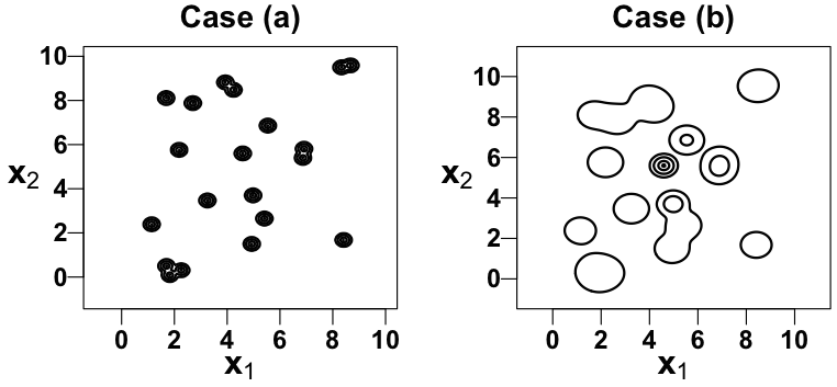
Figure 2: The first panel exhibits the contour plot of the target density in Example 1, case (a) and the second panel shows that of the target density in Example 1, case (b). The plotted contours outline regions with probability 1%, 10%, 50%, and 95% under $\pi(x)$.

Kou et al., (2006) used this target distribution to compare the equi-energy sampler (EE) and parallel tempering (PT). We follow their simulation configurations by running RAM for 75,000 iterations for both cases, initializing the chain at random values of $x^{(0)}$ and $z^{(0)}$ in the unit square. Although Kou et al., (2006) do not specify the burn-in size, we discard the first 25,000 iterations because they consistently use one third of the iterations as burn-in in the other examples. We set $q$ to be Gaussian with covariance matrix $\sigma^{2}I_{2}$, where $I_{2}$ is the identity matrix. To tune $\sigma$, we initilize ten independent chains with ten different values of $\sigma\in\{3.0,3.5,\ldots,7.5\}$. Following Kou et al., (2006), we set $\sigma$ to the value that leads to the best autocorrelation function among those that visit all modes. This is 4.0 in case (a) and $3.5$ in case (b). The acceptance rate is $0.048$ for case (a) and $0.228$ for case (b).

Fig. 3 gives bivariate scatterplots of the Monte Carlo sample of size 50,000 obtained with RAM for the two cases, bivariate trace plots of the last 2,000 iterations for case (a) and the last 1,000 iterations for case (b), and autocorrelation plots for $x_{1}$. Fig. 3 can be compared to Fig. 3 and Fig. 4 of Kou et al., (2006), which summarize the performance of EE and PT for cases (a) and (b), respectively.

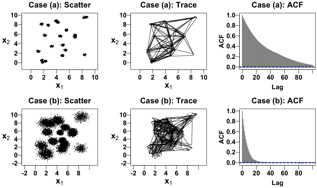
Figure 3: Results of the RAM algorithm. The first column displays bivariate scatterplots for 50,000 samples, the middle column displays the bivariate trace plots for the last 2,000 samples for case (a) and the last 1,000 samples for case (b), and the last column displays the autocorrelation functions for 50,000 samples of $x_{1}$.

To compare the accuracy of the moment estimates obtained with the algorithms, we again follow Kou et al., (2006) and run 20 independent chains using RAM. Table 2 summarizes the comparisons, where the ratios of the mean squared error (MSE) of both EE and PT to that of RAM are all greater than one. The improvement is particularly striking for case (b). These indicate that RAM leads to a more reliable proportion of iterations that are associated with each mode across the 20 runs.

Table 2: Moment estimates for cases (a) and (b) based on 20 independent chains, each of length 50,000, generated with RAM, EE (equi-energy sampler), and PT (parallel tempering). The results for EE and PT are from Kou et al., (2006), and presented in their original format: Sample average (sample standard deviation) over the 20 replications.

Case (a)	Truth	RAM	EE	PT	MSE ratio	MSE ratio
					(EE/RAM)	(PT/RAM)
$E(x_{1})$	$4.478$	$4.4708$ $(0.091)$	$4.5019$ $(0.107)$	$4.4185$ $(0.170)$	$1.44$	$3.89$
$E(x_{2})$	$4.905$	$4.9318$ $(0.101)$	$4.9439$ $(0.139)$	$4.8790$ $(0.283)$	$1.91$	$7.40$
$E(x^{2}_{1})$	$25.605$	$25.5717$ $(0.900)$	$25.9241$ $(1.098)$	$24.9856$ $(1.713)$	$1.61$	$4.09$
$E(x^{2}_{2})$	$33.920$	$33.2234$ $(1.100)$	$34.4763$ $(1.373)$	$33.5966$ $(2.867)$	$1.69$	$6.39$
Case (b)	Truth	RAM	EE	PT	MSE ratio	MSE ratio
					(EE/RAM)	(PT/RAM)
$E(x_{1})$	$4.688$	$4.673$ $(0.026)$	$4.699$ $(0.072)$	$4.709$ $(0.116)$	$5.89$	$15.42$
$E(x_{2})$	$5.030$	$5.029$ $(0.035)$	$5.037$ $(0.086)$	$5.001$ $(0.134)$	$6.07$	$15.33$
$E(x^{2}_{1})$	$25.558$	$25.508$ $(0.263)$	$25.693$ $(0.739)$	$25.813$ $(1.122)$	$7.87$	$18.47$
$E(x^{2}_{2})$	$31.378$	$31.456$ $(0.334)$	$31.433$ $(0.839)$	$31.105$ $(1.186)$	$6.01$	$12.59$

Finally, we compare the average evaluation cost of each algorithm by reporting the expected total number of evaluations of the target density $\pi$ needed to obtain the final sample, including burn-in, divided by the final sample size; we denote this quantity by $\textrm{N}_{\pi}^{\textrm{X}}$, where ‘X’ specifies the algorithm. As detailed in Appendix A, $\textrm{N}_{\pi}^{\textrm{EE}}=16.0$ and $\textrm{N}_{\pi}^{\textrm{PT}}=5.8$. For RAM, $\textrm{N}_{\pi}^{\textrm{RAM}}=7.1$ in case (a) and $\textrm{N}_{\pi}^{\textrm{RAM}}=5.0$ in case (b). More evaluations are needed for case (a) because the area of near zero density is much larger than that in case (b), see Fig. 2, and a forced uphill transition thus requires more proposals (and thus more evaluations). Nonetheless, the number of target density evaluations (and thus CPU time) required by RAM indicates that the gain of using RAM in terms of MSE is competitive.

3.2 Example 2: High-dimensional multimodal distributions

Consider an equal mixture of eight $d$-dimensional Gaussian distributions:

$$\pi(x)\propto\sum_{j=1}^{8}\exp\!\left(-\frac{1}{2}(x-\mu_{j})^{\top}(x-\mu_{j})\right)\!,$$ (11)

where $x=(x_{1},x_{2},\ldots,x_{d})^{\top}$ and the eight mean vectors are defined by setting their first three coordinates to the eight vertices of a cube of edge length ten situated with its corner at the origin and their remaining coordinates are filled with (10, 0) or (0, 10) repeatedly:

$$\begin{aligned} \mu_{1}=(10,10,10,{\color[rgb]{1,1,1}1}0,10,{\color[rgb]{1,1,1}1}0,10,...,{\color[rgb]{1,1,1}1}0,10),~{}~{}\mu_{2}=({\color[rgb]{1,1,1}1}0,{\color[rgb]{1,1,1}1}0,{\color[rgb]{1,1,1}1}0,10,{\color[rgb]{1,1,1}1}0,10,{\color[rgb]{1,1,1}1}0,...,10,{\color[rgb]{1,1,1}1}0),\\ \mu_{3}=(10,{\color[rgb]{1,1,1}1}0,10,{\color[rgb]{1,1,1}1}0,10,{\color[rgb]{1,1,1}1}0,10,...,{\color[rgb]{1,1,1}1}0,10),~{}~{}\mu_{4}=({\color[rgb]{1,1,1}1}0,10,10,{\color[rgb]{1,1,1}1}0,10,{\color[rgb]{1,1,1}1}0,10,...,{\color[rgb]{1,1,1}1}0,10),\\ \mu_{5}=({\color[rgb]{1,1,1}1}0,{\color[rgb]{1,1,1}1}0,10,{\color[rgb]{1,1,1}1}0,10,{\color[rgb]{1,1,1}1}0,10,...,{\color[rgb]{1,1,1}1}0,10),~{}~{}\mu_{6}=({\color[rgb]{1,1,1}1}0,10,{\color[rgb]{1,1,1}1}0,10,{\color[rgb]{1,1,1}1}0,10,{\color[rgb]{1,1,1}1}0,...,10,{\color[rgb]{1,1,1}1}0),\\ \mu_{7}=(10,{\color[rgb]{1,1,1}1}0,{\color[rgb]{1,1,1}1}0,10,{\color[rgb]{1,1,1}1}0,10,{\color[rgb]{1,1,1}1}0,...,10,{\color[rgb]{1,1,1}1}0),~{}~{}\mu_{8}=(10,10,{\color[rgb]{1,1,1}1}0,10,{\color[rgb]{1,1,1}1}0,10,{\color[rgb]{1,1,1}1}0,...,10,{\color[rgb]{1,1,1}1}0).\end{aligned}$$

Suppose that the first two modes, $\mu_{1}$ and $\mu_{2}$, are known, perhaps from an initial search, while the other six modes are unknown. Here, we investigate RAM’s ability to explore a high dimensional distribution by using it to sample (11) with the five values of $d\in\{3,5,7,9,11\}$. We also compare RAM to both Metropolis and PT, taking into account their average evaluation cost, $\textrm{N}_{\pi}^{\textrm{X}}$, as defined in Section 3.1.

We set $q$ to be a $d$-dimensional Gaussian density with covariance matrix $\Sigma$. To achieve a reasonable acceptance rate, we first run two Metropolis chains each of length 5,000, initialized at the two known mode locations and using a Gaussian jumping rule with covariance matrix $(2.38^{2}/d)\times I_{d}$, where $I_{d}$ is the identity matrix. We then set $\Sigma$ to the sample covariance matrix of the combined sample from the two chains. To improve Metropolis’ ability to jump between modes, we reset $\Sigma$ to the sample covariance matrix of the burn-in sample. This one-time adaptation does not affect the validity of the resulting chain.

For each $d$, we run RAM ten times to obtain ten chains each of length 500,000, discarding the first 200,000 iterations of each chain as burn-in. RAM’s average evaluation cost $\textrm{N}_{\pi}^{\textrm{RAM}}$ is 6.54 for $d=3$, 7.54 for $d=5$, 8.45 for $d=7$, 9.58 for $d=9$, and 10.77 for $d=11$. As $d$ increases, RAM requires more evaluations because it is more difficult to find a proposal that increases the density in the forced uphill transition.

For each $d$, we also obtain ten chains each using both Metropolis and PT with the same Gaussian jumping rule used by RAM. PT runs five parallel chains under five temperature levels, $2^{k}$ for $k=0,1,\ldots,4$, each of which uses Metropolis transitions. PT always proposes a single swap between a randomly chosen pair of chains under adjoining temperature levels at the end of each iteration. We determine the length of each chain and the burn-in size for Metropolis and PT by taking into account their average evaluation cost, denoted by $\textrm{N}^{\textrm{M}}_{\pi}$ and $\textrm{N}^{\textrm{PT}}_{\pi}$, respectively. For example, the length of each chain for Metropolis is 500,000$\times\textrm{N}^{\textrm{RAM}}_{\pi}/\textrm{N}^{\textrm{M}}_{\pi}$ and that for PT is 500,000$\times\textrm{N}^{\textrm{RAM}}_{\pi}/\textrm{N}^{\textrm{PT}}_{\pi}$ so that the (expected) total number of target density evaluations is the same for each algorithm. We need to adjust the burn-in size by the average evaluation cost for a fair comparison because a large burn-in size improves the effectiveness of the one-time adaptation.

We use two numerical measures to evaluate each algorithm. The first is the average number of the unknown modes that are discovered by each chain; we denote this by N${}_{\textrm{dis}}$ $(\leq 6)$. The second is the average frequency error rate (Kou et al.,, 2006), denoted by $\textrm{F}_{\textrm{err}}=\sum_{i=1}^{10}\sum_{j=1}^{8}|\textrm{F}_{i,j}-1/8|/80$, where $\textrm{F}_{i,j}$ is the proportion of iterations in chain $i$ whose nearest mode measured by the Euclidean distance is $\mu_{j}$.

Table 3: The sampling results include the length of each chain before discarding burn-in; the number of burn-in iterations; N_π = the average number of target density evaluations at each iteration; $\textrm{N}_{d}$ = the average number of downhill proposals for RAM; $\textrm{N}_{u}$ = the average number of uphill proposals for RAM; $\textrm{N}_{z}$ = the average number of downhill proposals for the auxiliary variable for RAM; acceptance rate; N${}_{\textrm{dis}}$ = the average number of the unknown modes that are discovered by each chain; and F${}_{\textrm{err}}=\sum_{i=1}^{10}\sum_{j=1}^{8}|\textrm{F}_{i,j}-1/8|/80$, where $\textrm{F}_{i,j}$ is the proportion of iterations in chain $i$ whose nearest mode is $\mu_{j}$.

$d$	Kernel	Length of a chain	$\textrm{N}_{\pi}$	Acceptance	N${}_{\textrm{dis}}$	F${}_{\textrm{err}}$
		(burn-in size)	($\textrm{N}_{d}$, $\textrm{N}_{u}$, $\textrm{N}_{z}$)	rate
$3$	Metropolis	3,272,000 (1,308,800)	1	0.036	6.0	0.021
	PT	2,467,429 2,(186,971)	7	0.025	6.0	0.025
	RAM	2,500,000 2,(200,000)	6.544	0.101	6.0	0.019
			(1.014, 4.210, 1.320)
$5$	Metropolis	3,768,500 (1,507,400)	1	0.019	6.0	0.047
	PT	2,538,357 2,(215,343)	7	0.041	6.0	0.041
	RAM	2,500,000 2,(200,000)	7.537	0.052	6.0	0.038
			(1.009, 5.222, 1.306)
$7$	Metropolis	4,220,500 (1,688,200)	1	0.014	5.8	0.209
	PT	2,602,929 2,(241,171)	7	0.058	6.0	0.058
	RAM	2,500,000 2,(200,000)	8.441	0.036	6.0	0.075
			(1.006, 6.136, 1.299)
$9$	Metropolis	4,734,000 (1,893,600)	1	0.012	5.6	0.312
	PT	2,676,286 2,(270,514)	7	0.075	6.0	0.075
	RAM	2,500,000 2,(200,000)	9.468	0.029	5.7	0.182
			(1.005, 7.171, 1.292)
$11$	Metropolis	5,350,000 (2,140,000)	1	0.023	5.3	0.512
	PT	2,764,286 2,(305,714)	7	0.004	6.0	0.108
	RAM	2,500,000 2,(200,000)	10.700	0.021	5.5	0.267
			(1.003, 8.416, 1.281)

Table 3 summarizes the results, and shows that using the same jumping rule, RAM is never worse than Metropolis in terms of $\textrm{N}_{\textrm{dis}}$ and $\textrm{F}_{\textrm{err}}$ regardless of dimension, and the improvement on $\textrm{F}_{\textrm{err}}$ can be substantial. It also shows that RAM’s $\textrm{F}_{\textrm{err}}$ starts off smaller than that of PT but deteriorates faster than PT’s once $d>5$, and that PT discovers all six modes for every $d$. This demonstrates the value of fine tuning particularly in higher dimensions for PT, including the number of parallel chains, temperature and proposal scale at each chain, and the number and rate of swaps at each iteration. Therefore, if one can afford the tuning cost, then PT has much to recommend it, especially in high dimensions.

3.3 Example 3: Sensor network localization

For high dimensional sampling, a blocked Gibbs sampler (Geman and Geman,, 1984) is sometimes more convenient and intuitive than direct Metropolis sampling. Here, we consider a realistic example from Ihler et al., (2005): Searching for unknown sensor locations within a network using the noisy distance data. This is called sensor network localization (Ihler et al.,, 2005; Lan et al.,, 2014). This problem is known to produce a high-dimensional, banana-shaped, and multimodal joint posterior distribution.

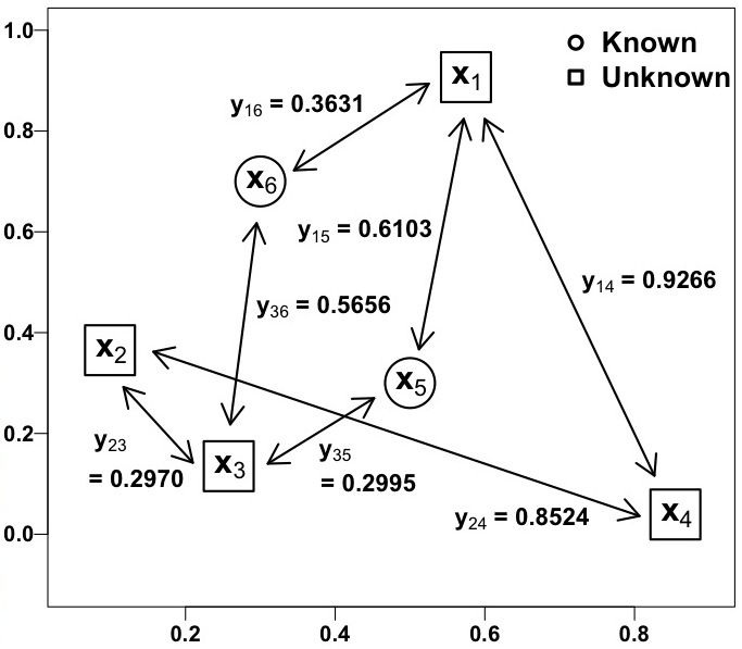
Figure 4: The simulated distances $y_{ij}~{}(=y_{ji})$ among the six stationary sensor locations, $x_{1},x_{2},\ldots,x_{6}$, are displayed if observed. The observation indicator $w_{ij}~{}(=w_{ji})$ is one if $y_{ij}$ is specified and is zero otherwise. The locations of the sensors are $x_{1}=(0.57,0.91)$, $x_{2}=(0.10,0.37)$, $x_{3}=(0.26,0.14)$, $x_{4}=(0.85,0.04)$, $x_{5}=(0.50,0.30)$, and $x_{6}=(0.30,0.70)$, where the first four locations, $x_{1}$, $x_{2}$, $x_{3}$, and $x_{4}$, are assumed to be unknown.

Modifying Lan et al., (2014)’s simulation setting, we suppose there are six stationary sensors scattered on a two dimensional space, and let $x_{k}^{\top}=(x_{k1},x_{k2})$ denote the two dimensional coordinates of the location of sensor $k$ for $k=1,2,\ldots,6$. We assume that the locations of the last two sensors, $x_{5}$ and $x_{6}$, are known and the locations of the other sensors, $x_{1},x_{2},x_{3}$, and $x_{4}$, are unknown parameters of interest. The Euclidean distance between two sensors, $x_{i}$ and $x_{j}$, denoted by $y_{ij}~{}(=y_{ji})$, is observed with a distance-dependent probability and Gaussian measurement error for $i=1,2,\ldots,5$ and $j=i+1,\ldots,6$. The probability distributions for the observed data are

$$w_{ij}\mid x_{1},\ldots,x_{4}~{}\sim\textrm{Bernoulli}\!\left(\exp\!\left(-\frac{\|x_{i}-x_{j}\|^{2}}{2\times 0.3^{2}}\right)\right)\!\\$$

and

$$y_{ij}\mid(w_{ij}=1),x_{1},\ldots,x_{4}~{}\sim\textrm{N}_{1}\!\left(\|x_{i}-x_{j}\|,~{}0.02^{2}\right)\!,$$

where $w_{ij}~{}(=w_{ji}$) is an indicator variable that equals one if the distance between $x_{i}$ and $x_{j}$ is observed. Simulated distances $y_{ij}$ are displayed in Fig. 4 where $w_{ij}=1$ if $y_{ij}$ is specified and zero otherwise. For each unknown location, we assume a diffuse bivariate Gaussian prior distribution with mean (0, 0) and covariance matrix $10^{2}\times I_{2}$. The eight dimensional likelihood function is thus

$$\begin{aligned} L(x_{1},x_{2},x_{3},x_{4})\propto&\prod_{j>i}\bigg{[}\exp\!\left(-\frac{(y_{ij}-\|x_{i}-x_{j}\|)^{2}}{2\times 0.02^{2}}\right)\\ &\times\exp\!\left(-\frac{w_{ij}\times\|x_{i}-x_{j}\|^{2}}{2\times 0.3^{2}}\right)\times\left(1-\exp\!\left(-\frac{\|x_{i}-x_{j}\|^{2}}{2\times 0.3^{2}}\right)\right)^{1-w_{ij}}\bigg{]}\end{aligned}$$

and the full posterior distribution is

$$\pi(x_{1},x_{2},x_{3},x_{4}\mid y,w)\propto L(x_{1},x_{2},x_{3},x_{4})\times\exp\left(-\frac{\sum_{k=1}^{4}x_{k}^{\top}x_{k}}{2\times 10^{2}}\right),$$ (12)

where $y=\{y_{ij},i>j\}$ and $w=\{w_{ij},i>j\}$. This model may suffer from non-identifiability when the number of observed distances is small because unknown locations appear in the likelihood only through distances; if $y_{ij}$ is observed between an unknown $x_{i}$ and a known $x_{j}$, the posterior distribution of $x_{i}$ may form a circle around $x_{j}$ without further observations.

We sample (12) using a Gibbs sampler by iteratively sampling the four bivariate conditionals denoted by $\pi_{i}(x_{i}\mid x_{j},j\not=i,y,w)$ for $i=1,2,3,4$. Since none of these is a standard distribution, we use Metropolis, RAM, or tempered transition (TT) (Neal,, 1996) kernels that are invariant with respect to each conditional distribution; see Appendix B for details of TT, jumping rules, and initial values. To sample $x_{k}$ from a RAM kernel that is marginally invariant to $\pi_{k}$, we must keep track of the auxiliary variable during the run, i.e., {$z^{(i)}_{k}$, $i=0,1,2,\ldots$}. At iteration $i$, we sequentially draw $x_{k}^{\prime}\sim q^{\textrm{D}}(x_{k}^{\prime}\mid x_{k}^{(i-1)})$, $x_{k}^{\ast}\sim q^{\textrm{U}}(x_{k}^{\ast}\mid x_{k}^{\prime})$, and $z_{k}^{\ast}\sim q^{\textrm{D}}(z_{k}^{\ast}\mid x_{k}^{\ast})$. We set $(x_{k}^{(i)},z_{k}^{(i)})$ to $(x_{k}^{\ast},z_{k}^{\ast})$ with probability $\alpha^{\textrm{J}}(x_{k}^{\ast},z_{k}^{\ast}\mid x_{k}^{(i-1)},z_{k}^{(i-1)})$ given in (8), and set $(x_{k}^{(i)},z_{k}^{(i)})$ to $(x_{k}^{(i-1)},z_{k}^{(i-1)})$ otherwise. Because {$z^{(i)}_{k}$, $i=0,1,2,\ldots$} are introduced solely to enable sampling $x_{k}$ from a RAM kernel, only $x_{k}^{(i)}$ is used to sample the other locations, and $z_{k}^{(i)}$ is used to draw $x_{k}^{(i+1)}$ at the next iteration.

For a fair comparison, we set the length of each chain to have the same average number of evaluations of $\pi_{i}$’s per iteration. As before, we use $\textrm{N}_{\pi}^{\textrm{X}}$ to denote the average evaluation cost. We first implement RAM within a Gibbs sampler for 220,000 iterations with the first 20,000 as burn-in, resulting in $\textrm{N}_{\pi}^{\textrm{RAM}}=36.13$, i.e., about nine density evaluations are required to sample each of the $\pi_{i}$’s (with caching). Since $\textrm{N}_{\pi}^{\textrm{M}}=4$ and $\textrm{N}_{\pi}^{\textrm{TT}}=24$ (with caching), we set the length of each Metropolis chain and TT chain respectively to 220,000$\times\textrm{N}_{\pi}^{\textrm{RAM}}/\textrm{N}_{\pi}^{\textrm{M}}$ and 220,000$\times\textrm{N}_{\pi}^{\textrm{RAM}}/\textrm{N}_{\pi}^{\textrm{TT}}$. However, unlike the previous example where there is a one-time adaption and hence it is important to adjust for the burn-in length as well, here we discard the first 20,000 iterations as burn-in for all three algorithms. This burn-in size is sufficient to remove the effect of random initial values of the algorithms.

Table 4: The sampling results summarize the length of each chain (including the 20,000 burn-in iterations); $\textrm{N}_{\pi}=$ the average number of evaluating $\pi_{1}$, $\pi_{2}$, $\pi_{3}$, and $\pi_{4}$ at each iteration; details of $\textrm{N}_{\pi}$ for each location; and the acceptance rates.

Kernel	Length of a chain	$\textrm{N}_{\pi}$	Details of $\textrm{N}_{\pi}$	Acceptance
			($\textrm{N}_{d}$, $\textrm{N}_{u}$, $\textrm{N}_{z}$)	rate
Metropolis	1,987,150	$\textrm{N}_{\pi}^{\textrm{M}}=4$	1 for each of $x_{1},\ldots,x_{4}$	0.00057 for $x_{1}$
				0.00151 for $x_{2}$
				0.00053 for $x_{3}$
				0.00115 for $x_{4}$
Tempered	331,192	$\textrm{N}_{\pi}^{\textrm{TT}}=24$	6 for each of $x_{1},\ldots,x_{4}$	0.00360 for $x_{1}$
transitions				0.01034 for $x_{2}$
				0.00369 for $x_{3}$
				0.00918 for $x_{4}$
RAM	220,000	$\textrm{N}_{\pi}^{\textrm{RAM}}=36.13$	9.40 for $x_{1}$ (1, 7.33, 1.07)	0.00349 for $x_{1}$
			8.64 for $x_{2}$ (1, 6.56, 1.08)	0.00830 for $x_{2}$
			9.22 for $x_{3}$ (1, 7.16, 1.06)	0.00353 for $x_{3}$
			8.87 for $x_{4}$ (1, 6.74, 1.13)	0.00730 for $x_{4}$

Table 4 summarizes the configurations of the samplers and their acceptance rates. RAM improves the acceptance rate of Metropolis by a factor at least of 5.5 given the same jumping rule without additional tuning. TT improves the acceptance rates even further by a factor of at least 6.3 (relative to Metropolis), but it requires additional tuning of the number of temperature levels, temperature, and jumping scale at each temperature level.

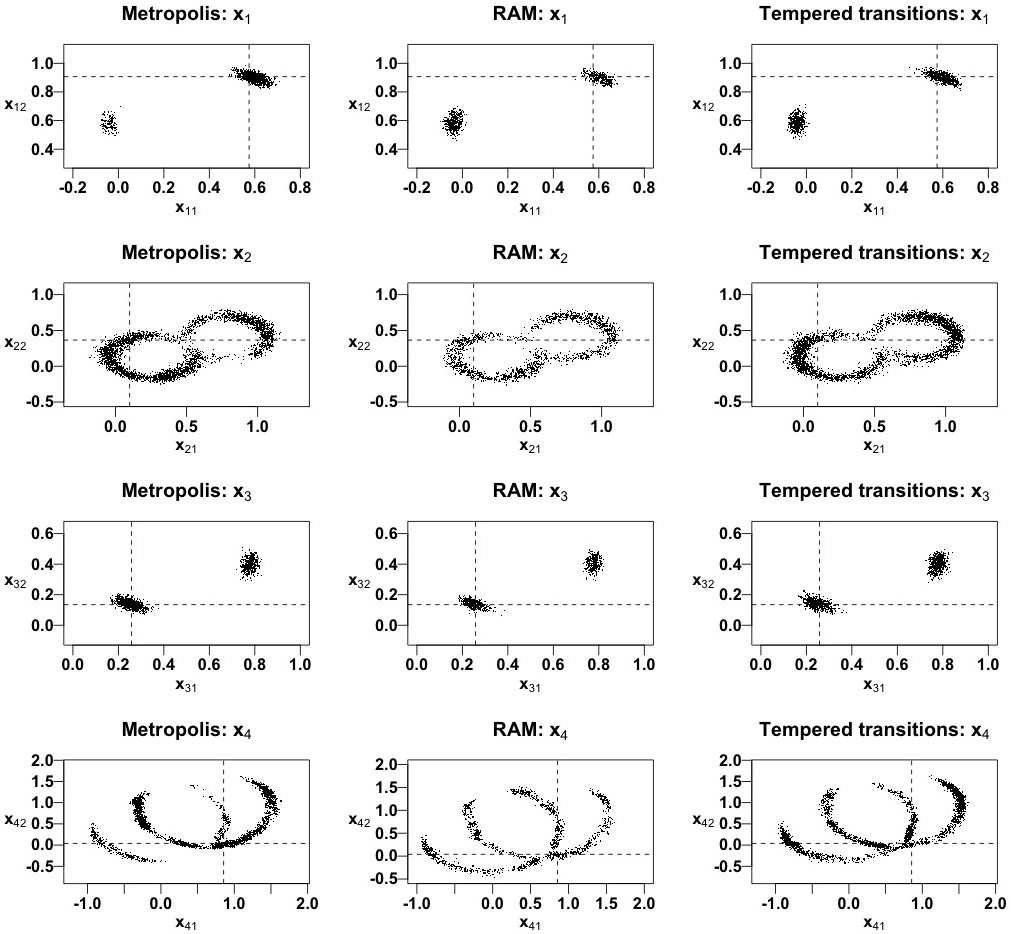
Figure 5: Scatterplots of the posterior sample of each location (rows) obtained by different samplers (column). The coordinates of the unknown sensors are denoted by dashed lines.

Fig. 5 gives scatterplots of the posterior samples of each unknown sensor location (rows) obtained by the three samplers (columns), where the dashed lines indicate the coordinates of the true location. The RAM sample is more dispersed than that of Metropolis, especially for $x_{1}$, $x_{2}$, and $x_{4}$, with the same jumping rule, and is as dispersed as that of TT without subtle tuning that TT requires. The posterior samples of both Metropolis and TT, however, are denser than that of RAM because of their larger sample sizes.

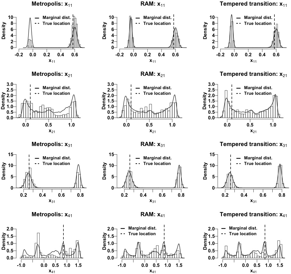
Figure 6: Histograms of the posterior sample of each first coordinate (rows) obtained by different kernels (columns). In each histogram, the marginal posterior density based on twenty million posterior samples obtained with each sampler is superimposed. The vertical dashed lines indicate the true sensor locations.

Fig. 6 compares the relative sizes of modes for the first coordinate of each unknown location (rows) obtained by each sampler (columns). In each histogram, we superimpose the marginal posterior density based on twenty million posterior draws obtained from each sampler after confirming that the shapes of the posterior densities obtained in this manner are almost identical for the three algorithms. The vertical dashed lines indicate the true sensor locations. RAM represents all four distributions better than Metropolis does, and it does as well as TT, but without the tuning requirement of the latter.

3.4 Example 4: Strong lens time delay estimation

Our final numerical illustration targets a multimodal distribution where one mode is extremely distant from the others. This multimodal distribution arises from the applied astrophysical problem that originally motivated the development of RAM; see Tak et al., (2017) for details. Here we review the problem and discuss a new efficient algorithm.

When there is a massive galaxy between a highly luminous quasar and the Earth, the gravitational field of the galaxy may act as a lens, bending the light emitted by the quasar. This may produce two (or more) slightly offset images of the quasar, an effect known as strong gravitational lensing (Schneider et al.,, 2006). There may be a time delay between the images in that their light follows different paths with different travel times. Thus, temporal features in time series of the brightness of each image appear shifted in time. The time delay is, for example, used to calculate the current expansion rate of the Universe, i.e., the Hubble constant (Refsdal,, 1964).

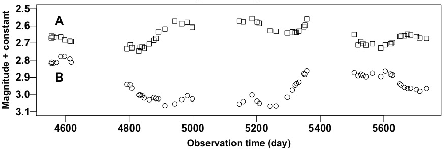
Figure 7: Two observed time series of doubly-lensed quasar Q0957+561 (Hainline et al.,, 2012). Time series $A$ is denoted by squares and time series $B$ is denoted by circles. Magnitude is an astronomical measure of brightness. Both time series are plotted with an offset (constant) in magnitude, but this does not affect the time delay estimation.

Fig. 7 displays two irregularly-observed time series of the brightness of the doubly-lensed quasar Q0957+561 (Hainline et al.,, 2012); the two time series are labeled $A$ and $B$. Brightness is reported on a magnitude scale where smaller values correspond to brighter images. Let $x\equiv\{x_{1},\ldots,x_{n}\}$ and $y\equiv\{y_{1},\ldots,y_{n}\}$ denote the $n$ magnitudes irregularly observed at time $t\equiv\{t_{1},\ldots,t_{n}\}$ in time series $A$ and $B$, respectively. Let $\delta\equiv\{\delta_{1},\ldots,\delta_{n}\}$ and $\eta\equiv\{\eta_{1},\ldots,\eta_{n}\}$ represent the $n$ known measurement standard deviations for $x$ and $y$, respectively. There are fifty seven observations in each time series, i.e., $n=57$.

We assume that for each observed time series there is an unobserved underlying brightness curve. Let $X(t)\equiv\{X(t_{1}),\ldots,X(t_{n})\}$ denote the latent magnitudes for time series $A$ and $Y(t)\equiv\{Y(t_{1}),\ldots,Y(t_{n})\}$ denote those for time series $B$. We further assume that one of the latent brightness curves is a shifted version of the other, i.e.,

$$Y(t_{j})=X(t_{j}-\Delta)+\beta_{0},$$ (13)

where $\Delta$ is the unknown time delay and $\beta_{0}$ is an unknown magnitude offset.

The observed magnitudes given the latent magnitudes are assumed to be independent Gaussian variables:

$$x_{j}\mid X(t_{j})\sim\textrm{N}_{1}\!\left(X(t_{j}),~{}\delta^{2}_{j}\right)\!\quad\textrm{and}\quad y_{j}\mid Y(t_{j})\sim\textrm{N}_{1}\!\left(Y(t_{j}),~{}\eta^{2}_{j}\right)\!.$$ (14)

Using (13), we can express the model for $y$ in (14) as

$$y_{j}\mid X(t_{j}-\Delta),\Delta,\beta_{0}\sim\textrm{N}_{1}\!\left(X(t_{j}-\Delta)+\beta_{0},~{}\eta^{2}_{j}\right)\!.$$ (15)

We assume $X(\cdot)$ follows an Ornstein-Uhlenbeck process (Kelly et al.,, 2009). Solving the resulting stochastic differential equation yields the sampling distribution of $X(t^{\Delta})$, where $t^{\Delta}\equiv(t^{\Delta}_{1},\ldots,t^{\Delta}_{2n})^{\top}$ contains the sorted $2n$ times among the $n$ observation times, $t$, and the $n$ time-delay-shifted observation times, $t-\Delta$. Specifically,

$$\begin{aligned} X(t_{1}^{\Delta})\mid\Delta,\theta&~{}\sim~{}\textrm{N}_{1}\!\left(\mu,~{}\frac{\tau\phi^{2}}{2}\right)\!,~{}~{}~{}\textrm{and for}~{}j=2,3,\ldots,2n,\\ ~{}~{}X(t_{j}^{\Delta})\mid X(t_{j-1}^{\Delta}),\Delta,\theta&~{}\sim~{}\textrm{N}_{1}\!\left(\mu+a_{j}\big{(}X(t_{j-1}^{\Delta})-\mu\big{)},~{}\frac{\tau\phi^{2}}{2}(1-a^{2}_{j})\right)\!,\end{aligned}$$ (16)

where $\theta\equiv(\mu,\phi^{2},\tau)^{\top}$ and $a_{j}=\exp(-(t^{\Delta}_{j}-t^{\Delta}_{j-1})/\tau)$.

Following Tak et al., (2017), we set independent priors for the model parameters:

$$\begin{aligned} \Delta&\sim\textrm{Uniform}[-1178.939,~{}1178.939],~{}\beta_{0}\sim\textrm{Uniform}[-60,60],\\ \mu&\sim\textrm{Uniform}[-30,30],~{}\phi^{2}\sim\textrm{inverse-Gamma}(1,2/10^{7}),~{}\tau\sim\textrm{inverse-Gamma}(1,1).\end{aligned}$$ (17)

The resulting joint posterior density function is

$$\begin{aligned} \pi(X(t^{\Delta}),\Delta,\beta_{0},\theta\mid x,y)\propto&\left[\prod_{j=1}^{n}f_{1}\!\left(x_{j}\mid X(t_{j})\right)\times f_{2}\!\left(y_{j}\mid X(t_{j}-\Delta),\Delta,\bm{\beta}\right)\right]\\ \times~{}g(X(t^{\Delta}_{1})\mid\Delta,\bm{\theta})&\times\left[\prod_{j=2}^{2n}g(X(t^{\Delta}_{j})\mid X(t^{\Delta}_{j-1}),\Delta,\bm{\theta})\right]\times h(\Delta,\beta_{0},\theta),\end{aligned}$$ (18)

where the density functions, $f_{1}$, $f_{2}$, $g$, and $h$ are defined by (14)–(17), respectively.

Table 5: A Metropolis-Hastings within Gibbs sampler for the time delay model. We draw $\Delta$ from a kernel that is invariant to $\pi_{11}$ and draw $X(t^{\Delta})$ from $\pi_{12}$ if $\Delta$ is newly updated.

Set initial values $\Delta^{(0)}$, $X^{(0)}(t^{\Delta^{(0)}})$, $\beta_{0}^{(0)}$, and $\theta^{(0)}$. For $i=1,2,\ldots$,

Step 1: Draw $\left(X^{(i)}(t^{\Delta^{(i)}}),\Delta^{(i)}\right)\sim\pi_{1}\left(X(t^{\Delta}),\Delta\mid\beta^{(i-1)}_{0},\theta^{(i-1)}\right)$

= $\pi_{11}\left(\Delta\mid\beta^{(i-1)}_{0},\theta^{(i-1)}\right)\pi_{12}\left(X(t^{\Delta})\mid\Delta,\beta^{(i-1)}_{0},\theta^{(i-1)}\right).$

Step 2: Draw $\beta^{(i)}_{0}\sim\pi_{2}\left(\beta_{0}\mid\theta^{(i-1)},X^{(i)}(t^{\Delta^{(i)}}),\Delta^{(i)}\right)$.

Step 3: Draw $\theta^{(i)}\sim\pi_{3}\left(\theta\mid X^{(i)}(t^{\Delta^{(i)}}),\Delta^{(i)},\beta^{(i)}_{0}\right).$

To sample from (18), we adopt an MH within Gibbs sampler (Tierney,, 1994) composed of the three steps shown in Table 5; see Appendices A–C of Tak et al., (2017) for details. We suppress conditioning on $x$ and $y$ here and elsewhere. Because we cannot directly sample $\pi_{11}(\Delta\mid\beta_{0},\theta)$ in Step 1 and the marginal posterior distribution of $\Delta$ is often multimodal, we draw $\Delta$ using one of four algorithms: (i) Metropolis, (ii) Metropolis with a mixture jumping rule, (iii) RAM, or (iv) TT. The mixture jumping rule generates a proposal from the Gaussian jumping rule used by Metropolis with probability 0.5 and from the prior distribution of $\Delta$ otherwise. To sample $\Delta$ using the RAM kernel, we additionally keep track of the auxiliary variable during the run, i.e., {$z^{(i)}$, $i=0,1,2,\ldots$}. At iteration $i$, we draw $\Delta^{\prime}\sim q^{\textrm{D}}(\Delta^{\prime}\mid\Delta^{(i-1)})$, $\Delta^{\ast}\sim q^{\textrm{U}}(\Delta^{\ast}\mid\Delta^{\prime})$, and $z^{\ast}\sim q^{\textrm{D}}(z^{\ast}\mid\Delta^{\ast})$ sequentially. We set $(\Delta^{(i)},z^{(i)})$ to $(\Delta^{\ast},z^{\ast})$ with probability $\alpha^{\textrm{J}}(\Delta^{\ast},z^{\ast}\mid\Delta^{(i-1)},z^{(i-1)})$ given in (8), and set $(\Delta^{(i)},z^{(i)})$ to $(\Delta^{(i-1)},z^{(i-1)})$ otherwise. Because {$z^{(i)}$, $i=0,1,2,\ldots$} are introduced solely to enable sampling $\Delta$ from the RAM kernel, only $\Delta^{(i)}$ is used to sample $X(t^{\Delta})$, $\beta_{0}$, and $\theta$ in the other steps in Table 5, and $z^{(i)}$ is used to draw $\Delta^{(i+1)}$ at the next iteration.

Specifically, we fit the time delay model using the MH within Gibbs sampler equipped with TT for $\Delta$ first, initiating a single long chain of length 5,050,000 at the center of the entire range of $\Delta$, i.e., $\Delta^{(0)}=0$. We set the initial values of the other parameters as follows; $\beta_{0}^{(0)}=\sum_{j=1}^{n}\{y_{j}-x_{j}\}/n=-0.113$, $\mu^{(0)}=\sum_{j=1}^{n}x_{j}/n={2.658}$, $\phi^{(0)}=0.01$, $\tau^{(0)}=200$, and $X^{(0)}(t^{\Delta^{(0)}})$ is a vector of $x$ and $y-\beta_{0}^{(0)}$ that are sorted in time, $t$ for $x$ and $t-\Delta$ for $y-\beta_{0}^{(0)}$. Multiple initial values spread across the entire range result in nearly identical posterior distributions. We discard the first 50,000 draws as burn-in. For the tuning parameters of TT, we set five temperature levels, $T_{j}=4^{j}$ for $j=1,\ldots,5$, and corresponding jumping scales for Metropolis updates, $\sigma_{j}=500\times 1.2^{j-1}$, so that $\sigma_{5}$ (= 1,037) is about a half of the length of the range of $\Delta$. Using the same initial values ($z^{(0)}=\Delta^{(0)}$ for RAM), we obtain an additional chain using each of the MH within Gibbs sampler equipped with Metropolis, RAM, and Metropolis with a mixture jumping rule. In all these cases, we set $q$ to be Gaussian with $\sigma=700$, i.e., about one third length of the entire range and similar to the jumping scale of TT at the middle temperature level ($\sigma_{3}=720$). This value of $\sigma$ should be advantageous to Metropolis because it roughly equals the distance between the modes. Since Metropolis, RAM, and Metropolis with a mixture jumping rule take less CPU time than TT, we run longer chains of the three algorithms to match the CPU time, discarding the first 50,000 iterations of each as burn-in; see Appendix C for details of the average number of $\pi_{11}$ evaluations.

Table 6: The length of a chain including burn-in; acceptance rate for $\Delta$; and $\textrm{N}_{\textrm{jumps}}$ = the total number of jumps between the two distant modes during the post burn-in run.

	Length of	Acceptance	$\textrm{N}_{\textrm{jumps}}$
	a chain	rate
i(i)i Metropolis	22,266,816	0.0150	144
i​(ii)i​ Metropolis with mixture jumping rule	19,710,188	0.0129	190
(iii) RAM	7,111,612	0.0508	326
(iv) Tempered transitions	5,050,000	0.3022	311

Table 6 summarizes the results from running each algorithm for nearly the same CPU time (28,352 seconds). Overall, given the same jumping rule and without additional tuning, RAM improves upon both versions of Metropolis; the total number of jumps between the two distant modes in the post burn-in sample, denoted by $\textrm{N}_{\textrm{jumps}}$, is at least 1.7 times higher for RAM, and RAM’s acceptance rate is at least 3.4 times higher. With additional tuning of the number of rungs, temperature, and jumping scale, TT performs no better than RAM in terms of $\textrm{N}_{\textrm{jumps}}$ but its acceptance rate is about 5.9 times higher than Metropolis.

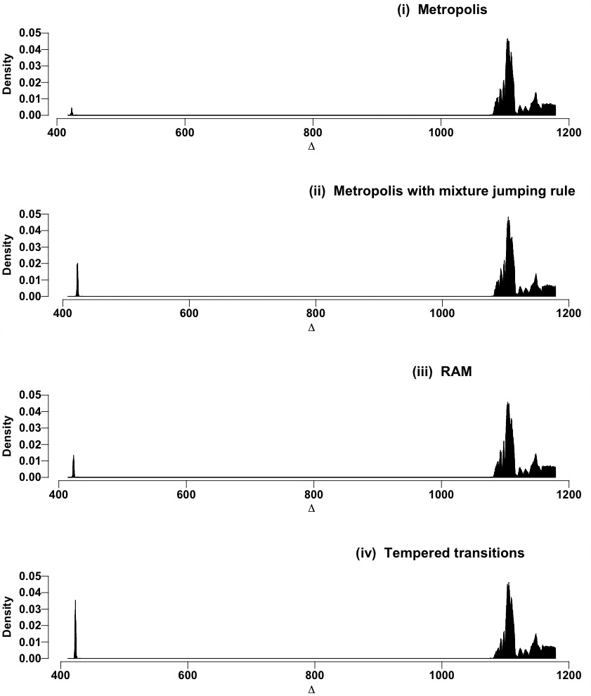
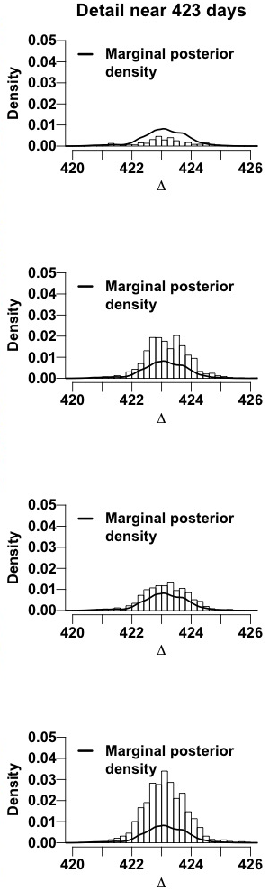
Figure 8: Results of running the algorithms for nearly the same CPU time. The rows represent the four samplers. The first column displays the histograms based on the posterior sample of $\Delta$ and the second column focuses on the mode near 423 days. In the second column, we superimpose the posterior density of $\Delta$ obtained by an oracle sampler (assuming the mode locations are known) to check the reliability of the relative sizes of the modes.

The first column of Fig. 8 displays histograms of the posterior sample of $\Delta$ obtained using the four different kernels. The size of the mode near 423 days, which is of great scientific interest, differs substantially among the samplers. In the second column of Fig. 8, we magnify this mode, superimposing a curve that represents the marginal posterior density of $\Delta$ based on twenty million posterior samples obtained with an oracle sampler constructed with knowledge of both mode locations. The size and shape of the mode near 423 days obtained with RAM match the oracle sampler better than the other algorithms, which is an algorithmic confirmation of the reliability of RAM.

4 Concluding remarks

We propose RAM both as an alternative to deal with multimodality, and as a newer strategy of forming acceptance probabilities. It can also be viewed as using negative temperature in annealing type of strategies, as Professor Art Owen recognized in his comments on an early version of our paper.

More work is needed to extend RAM’s applicability. In particular, we plan to compare the theoretical convergence rate of our algorithm to others, but this is difficult partially owing to the intractable down-up jumping density, $q^{\textrm{DU}}$. Also, a better set of strategies for tuning RAM in various multimodal cases needs to be investigated. Different ways to encourage a down-up movement in density may exist, e.g., mixing anti-Langevin and Langevin algorithms or tempering with negative and positive temperature levels, both of which were suggested in a personal blog of Professor Christian P. Robert. Another avenue for further improvement is to apply the ideas of the mode-jumping proposal and the delayed rejection method to RAM, e.g., allowing an asymmetric density function $q$ so that the downhill move encourages longer jumps than the uphill move does. Using this down-up idea to construct a global optimizer is another possible extension as the tempering idea is used for a statistical annealing. We invite interested readers to explore these possibilities.

Supplementary materials

Appendices:

Appendices A, B, and C as cited in the article (Appendices.pdf).

R code and data:

All the R code and data used in this article (RAM.zip).

Acknowledgements
This project was conducted under the auspices of the CHASC International Astrostatistics Center. CHASC is supported by the NSF grants DMS 1208791, 1209232, 1513484, 1513492, and 1513546. Xiao-Li Meng acknowledges partial financial support from the NSF grants given to CHASC. Hyungsuk Tak acknowledges partial support from the NSF grant DMS 1127914 given to SAMSI. David A. van Dyk acknowledges support from a Wolfson Research Merit Award (WM110023) provided by the British Royal Society and from a Marie-Curie Career Integration Grant (FP7-PEOPLE-2012-CIG-321865) provided by the European Commission. The authors thank the associate editor and two referees for their insightful comments and suggestions that significantly improved the presentation. We also thank Christian P. Robert, Pierre E. Jacob, Art B. Owen, and Natesh S. Pillai for very helpful discussions and Steven R. Finch for his proofreading.

Appendix A The average number of density evaluations in Section 3.1

Kou et al., (2006) implement the EE (equi-energy) sampler by running five parallel chains under five different temperature levels. The chain under the highest temperature adopts only MH transitions, and the other four chains use an EE jump with probability 0.1 and an MH transition otherwise at each iteration. The EE sampler begins by running a chain under the highest temperature for 75,000 iterations; the first 25,000 are burn-in iterations and the next 50,000 iterations form an energy ring at the highest temperature. The first chain uses only MH transitions. After running the first chain for 75,000 iterations, the sampler initiates the next chain under the second highest temperature and runs it for 75,000 iterations; the first 25,000 are burn-in iterations and the next 50,000 iterations form an energy ring at the second highest temperature. From the second chain, the sampler adopts an EE jump with probability 0.1 and an MH transition otherwise at each iteration. This process continues until the EE sampler finishes running the fifth chain under the unit temperature for 75,000 iterations; the first 25,000 iterations are discarded. All chains keep running until the end of the fifth chain, which means that the first chain runs for $5\times$75,000 iterations in total and the second one runs for $4\times$75,000 iterations, etc. Each EE jump needs to evaluate the target density twice (with caching). Thus, the (expected) total number of the density evaluations is $16\times$75,000 and that per iteration is 16.0.

Similarly, Kou et al., (2006) implement parallel tempering with five temperature levels and propose four swaps with probability 0.1 at the end of each iteration. Five chains under five different temperature levels are run simultaneously for 75,000 iterations, using MH transitions. At the end of each iteration, four swaps occur with probability 0.1 and no swaps otherwise. Each swap requires two additional evaluations of the target (with caching). Thus, the (expected) total number of the target density evaluations is 435,000 and the average number of the density evaluations per iteration is 5.8 (=435,000/75,000).

Appendix B Implementation details in Section 3.3

Tempered transitions require several tuning parameters, e.g., the number of rungs of the temperature ladder and the temperature and jumping scale of each rung, and setting these parameters is known to be challenging in practice (Behrens et al.,, 2012). At each iteration, the tempered transitions ascend the temperature ladder to explore a flatter surface where the modes are melted down, and then descend the ladder, accepting the last candidate with a modified acceptance probability to maintain the stationary distribution (Neal, 1996). To sample $\pi_{1}$ in (12) at iteration $i$, for example, suppose ${\pi_{1j}(x_{1})\propto\{\pi_{1}(x_{1}\mid x_{2}^{(i-1)},x_{3}^{(i-1)},x_{4}^{(i-1)},y,w)\}^{1/T_{j}}}$, where $T_{j}$ is the temperature at rung $j$ for $j=1,\ldots,J$. The target density is $\pi_{10}(x_{1})$ and the ladder has $J$ rungs with $T_{0}=1<T_{1}<\cdots<T_{J}$. Within each iteration $i$, starting from $j=1$ to $J$, we generate $\hat{x}_{1j}$ from $\textrm{N}_{2}(\hat{x}_{1,j-1},\Sigma_{j})$, where $\hat{x}_{10}=x_{1}^{(i-1)}$, and accept it with probability $\min\{1,\pi_{1j}(\hat{x}_{1j})/\pi_{1j}(\hat{x}_{1,j-1})\}$ and set $\hat{x}_{1j}=\hat{x}_{1,j-1}$ otherwise. Once we reach $j=J$, we reverse the process from $j=J$ to $1$ and generate $\check{x}_{1,j-1}$ from $\textrm{N}_{2}(\check{x}_{1j},\Sigma_{j})$ where $\check{x}_{1J}=\hat{x}_{1J}$, and accept it with probability $\min\{1,\pi_{1,j-1}(\check{x}_{1,j-1})/\pi_{1,j-1}(\check{x}_{1j})\}$ and set $\check{x}_{1,j-1}=\check{x}_{1j}$ otherwise until we reach the bottom of the temperature ladder, collecting $\check{x}_{1,J-1},\ldots,\check{x}_{10}$. After generating the last proposal $\check{x}_{10}$, we set $x_{1}^{(i)}=\check{x}_{10}$ with an MH acceptance probability of

$$\min\left\{1,~{}~{}\frac{\pi_{11}(x_{1}^{(i-1)})}{\pi_{10}(x_{1}^{(i-1)})}\times\cdots\times\frac{\pi_{1J}(\hat{x}_{1,J-1})}{\pi_{1,J-1}(\hat{x}_{1,J-1})}\frac{\pi_{1,J-1}(\check{x}_{1,J-1})}{\pi_{1J}(\check{x}_{1,J-1})}\times\cdots\times\frac{\pi_{10}(\check{x}_{10})}{\pi_{11}(\check{x}_{10})}\right\},$$

and set $x_{1}^{(i)}=x_{1}^{(i-1)}$ otherwise.

To fit the simulated data, we set three rungs with temperature equal to $2^{j}$ for the $j$th rung. Because the longest observed distance between two sensors is about 0.9, we set the jumping covariance matrix $\Sigma_{j}=(0.9\times 1.2^{j-1})^{2}\times I_{2}$ for each Metropolis update of the tempered transitions for the $j$th rung. For Metropolis and RAM, we set $\Sigma=1.08^{2}\times I_{2}$. This is the same as the jumping covariance matrix of tempered transitions at the middle rung, i.e., $\Sigma_{2}$. An initial value for each unknown location for each Markov chain is randomly selected from the unit square, $[0,1]\times[0,1]$.

Appendix C The average number of $\pi_{11}$ evaluations in Section 3.4

Since the kernels are used only to sample $\pi_{11}$ in Step 1 of Table 5, the average number of $\pi_{11}$ evaluations at each iteration ($\textrm{N}_{\pi_{11}}$) is not proportional to the entire CPU time needed for sampling the full posterior $\pi$ in (18). For reference, $\textrm{N}^{\textrm{M}}_{\pi_{11}}=2$ (with either the Gaussian or mixture proposal), $\textrm{N}^{\textrm{RAM}}_{\pi_{11}}=8.76$ ($\textrm{N}_{d}=1$, $\textrm{N}_{u}=4.48$, $\textrm{N}_{z}=1.28$), and $\textrm{N}^{\textrm{TT}}_{\pi_{11}}=11$. Each Metropolis transition evaluates $\pi_{11}$ twice, once for the current state and once for the proposal at each iteration. Caching the density value of the current state does not help reduce $\textrm{N}_{\pi_{11}}$ because the density of the current state changes according to the updates of the other parameters in Steps 2 and 3 of Table 5.

References

- Andrieu and Roberts, (2009) Andrieu, C. and Roberts, G. O. (2009). The Pseudo-Marginal Approach for Efficient Monte Carlo Computations. The Annals of Statistics, 37(2):697–725.
- Beaumont, (2003) Beaumont, M. A. (2003). Estimation of Population Growth or Decline in Genetically Monitored Populations. Genetics, 164(3):1139–1160.
- Behrens et al., (2012) Behrens, G., Friel, N., and Hurn, M. (2012). Tuning Tempered Transitions. Statistics and Computing, 22(1):65–78.
- Chib and Greenberg, (1995) Chib, S. and Greenberg, E. (1995). Understanding the Metropolis-Hastings Algorithm. The American Statistician, 49(4):327–335.
- Geman and Geman, (1984) Geman, S. and Geman, D. (1984). Stochastic Relaxation, Gibbs distributions, and the Bayesian Restoration of Images. IEEE Transactions on Pattern Analysis and Machine Intelligence, 6:721–741.
- Geyer, (1991) Geyer, C. J. (1991). Markov chain Monte Carlo Maximum Likelihood. Computing Science and Statistics: Proceedings of the 23rd Symposium on the Interface, 156–163.
- Geyer and Thompson, (1995) Geyer, C. J. and Thompson, E. A. (1995). Annealing Markov chain Monte Carlo with Applications to Ancestral Inference. Journal of the American Statistical Association, 90(431):909–920.
- Hainline et al., (2012) Hainline, L. J., Morgan, C. W., Beach, J. N., Kochanek, C., Harris, H. C., Tilleman, T., Fadely, R., Falco, E. E., and Le, T. X. (2012). A New Microlensing Event in the Doubly Imaged Quasar Q0957+561. The Astrophysical Journal, 744(2):104–113.
- Hastings, (1970) Hastings, W. K. (1970). Monte Carlo Sampling Methods using Markov Chains and Their Applications. Biometrika, 57(1):97–109.
- Ihler et al., (2005) Ihler, A. T., Fisher, J. W., Moses, R. L., and Willsky, A. S. (2005). Nonparametric Belief Propagation for Self-Localization of Sensor Networks. IEEE Journal on Selected Areas in Communications, 23(4):809–819.
- Kelly et al., (2009) Kelly, B. C., Bechtold, J., and Siemiginowska, A. (2009). Are the Variations in Quasar Optical Flux Driven by Thermal Fluctuations? The Astrophysical Journal, 698(1):895–910.
- Kou et al., (2006) Kou, S. C., Zhou, Q., and Wong, W. H. (2006). Discussion Paper: Equi-Energy Sampler with Applications in Statistical Inference and Statistical Mechanics. The Annals of Statistics, 34(4):1581–1619.
- Lan et al., (2014) Lan, S., Streets, J., and Shahbaba, B. (2014). Wormhole Hamiltonian Monte Carlo. Proceedings of the AAAI Conference on Artificial Intelligence, 2014:1953–1959.
- Metropolis et al., (1953) Metropolis, N., Rosenbluth, A. W., Rosenbluth, M. N., Teller, A. H., and Teller, E. (1953). Equation of State Calculations by Fast Computing Machines. The Journal of Chemical Physics, 21(6):1087–1092.
- Møller et al., (2006) Møller, J., Pettitt, A. N., Reeves, R., and Berthelsen, K. K. (2006). An Efficient Markov Chain Monte Carlo Method for Distributions with Intractable Normalising Constants. Biometrika, 93(2):451–458.
- Neal, (1996) Neal, R. M. (1996). Sampling From Multimodal Distributions Using Tempered Transitions. Statistics and Computing, 6(4):353–366.
- R Core Team, (2016) R Core Team (2016). R: A Language and Environment for Statistical Computing. R Foundation for Statistical Computing, Vienna, Austria.
- Refsdal, (1964) Refsdal, S. (1964). The Gravitational Lens Effect. Monthly Notices of the Royal Astronomical Society, 128:295–306.
- Schneider et al., (2006) Schneider, P., Wambsganss, J., and Kochanek, C. (2006). Gravitational Lensing: Strong, Weak and Micro. Springer-Verlag, New York.
- Tak et al., (2017) Tak, H., Mandel, K., van Dyk, D. A., Kashyap, V. L., Meng, X.-L., and Siemiginowska, A. (2017). Bayesian Estimates of Astronomical Time Delays between Gravitationally Lensed Stochastic Light Curves. The Annals of Applied Statistics, 11(3):1309–1348.
- Tierney, (1994) Tierney, L. (1994). Markov Chains for Exploring Posterior Distributions. The Annals of Statistics, 22(4):1701–1728.
- Tierney and Mira, (1999) Tierney, L. and Mira, A. (1999). Some Adaptive Monte Carlo Methods for Bayesian Inference. Statistics in Medicine, 18(1718):2507–2515.
- Tjelmeland and Hegstad, (2001) Tjelmeland, H. and Hegstad, B. K. (2001). Mode Jumping Proposals in MCMC. Scandinavian Journal of Statistics, 28(1):205–223.
- Trias et al., (2009) Trias, M., Vecchio, A., and Veitch, J. (2009). Delayed Rejection Schemes for Efficient Markov-Chain Monte-Carlo Sampling of Multimodal Distributions. arXiv preprint arXiv:0904.2207.