Chaplygin Gas Hořava-Lifshitz Quantum Cosmology

Abstract

In this paper, we study the Chaplygin gas Hořava-Lifshitz quantum cosmology. Using Schutz formalism and Arnowitt-Deser-Misner decomposition, we obtain the corresponding Schrödinger-Wheeler-DeWitt equation. We obtain exact classical and quantum mechanical solutions and construct wave packets to study the time evolution of the expectation value of the scale factor for two cases. We show that unlike classical solutions and upon choosing appropriate initial conditions, the expectation value of the scale factor never tends to the singular point which exhibits the singularity-free behavior of the solutions in the quantum domain.

I Introduction

In recent years, the results from supernova Ia have shown that the expansion of our Universe is accelerating unlike the Friedmann-Robertson-Walker (FRW) cosmological models with nonrelativistic matter and radiation C1 ; C2 ; C3 . Also, the cosmic background radiation data imply that our Universe is in positively accelerated state C4 ; C5 ; C6 . The cosmological constant $\Lambda$ as the usual vacuum energy may be responsible for this accelerating evolution of the Universe with the negative pressure. Unfortunately, the measured value of the cosmological constant is 120 orders of magnitude smaller than its theoretical predicted value C7 ; C8 .

On the other hand, thr Chaplygin gas, as a perfect fluid which behaves like a pressureless fluid at early times and a cosmological constant at later times, can be a candidate for the dark energy ch_gas2 ; Benaoum ; ZXL ; visc . The generalized Chaplygin gas with negative pressure is described by an exotic equation of state,

$$p=-\frac{A}{\rho^{\alpha}},$$ (1)

where $A$ is a positive parameter, $p$ is the pressure, $\rho$ is the energy density, and $\alpha$ is a positive parameter so that $0<\alpha\leq 1$. In the standard model of Chaplygin gas, we set $\alpha=1$ ch_gas4 . Recently, various studies have been done in the literature, such as cosmology with the Chaplygin gas to explain the transition from a dust-dominated Universe to the accelerating expansion stage ch_gas1 ; ch_gas4 , modified generalized Chaplygin gas MCG1 ; MCG2 ; MCG3 , modified cosmic Chaplygin gas MCCG1 ; MCCG2 , and phenomenological relations between brane-world scenarios and FRW minisuperspace cosmologies in the presence of the generalized Chaplygin gas BLM .

The idea of an early Chaplygin gas phase in the Universe was first suggested in Refs. BLM ; L20 ; L21 and later extended in Refs. L22 ; L23 ; L24 . It is interesting to note that the generalized Chaplygin gas has a connection with string theory. It can be effectively obtained in the light cone parametrization from the Nambu-Goto action for a $d$-brane in a ($d+1$,1)-dimensional spacetime J25 . This motivates the application of the generalized Chaplygin gas model at early time in the evolution of the Universe. In particular, the Chaplygin inflation is addressed in Ref. L20 and the tachyon-Chaplygin inflationary Universe is studied in Ref. J27 .

In fact, Chaplygin spacetime models are related to a generalized Born-Infeld action with a complex scalar field which corresponds to a perturbed $d$-brane in a ($d+1$,1)-dimensional spacetime ch_gas2 ; ch_gas1 ; x31 . A generalized Born-Infeld phantom inspired generalized Chaplygin gas model is presented in Ref. x30 . This opens a window to investigate brane-world physics based on a phenomenological point of view. Brane-world scenarios could explain various cosmological effects such as the inflation based on the WMAP data C5 , the origin of our Universe, and other fundamental issues such as the hierarchy problem x34 . The quantum cosmological creation of brane-world models is also addressed in Refs. x37 ; x42 ; x43 ; x44 ; x45 ; x46 ; x47 ; x48 . This allows us to use the similarities between the quantum cosmology of a brane-world model and the Chaplygin gas quantum cosmology.

Recently, a single-field inflation scenario is presented in Ref. JCAP where the properties of the inflaton field areequivalent to a generalized Chaplygin gas. Based on the measurements released by the Planck data and the WMAP large-angle polarization, it is found that the $\alpha$ parameter is given by $\alpha=0.2578\pm 0.0009$ JCAP ; alpha ; comment . In Ref. Lopez2013 , a slow-roll inflationary scenario is modeled by a generalized Chaplygin gas that can interpolate between a network of frustrated topological defects and a de Sitter-like or a power-law inflationary era.

After the Universe reached the dust-dominated stage, the exponentially expanding evolution of the Universe represents a quantum mechanical transition with some remnant component of the original wave function of the Universe BLM . In fact, there is a quantum mechanical background behind the classically observed Universe on large scales during the dust dominance epoch which is based on the cosmological influence of a rapidly oscillating wave function with a small amplitude. This wave function remnant can be considered as a robust component with respect to decoherence processes in the early times x49 ; x50 ; x51 ; x52 .

In 1970, Schutz introduced a velocity potential representation for the four-velocity of a perfect fluid in general relativity schutz1 . The equations of hydrodynamics for a perfect fluid are expressed in terms of six scalar potentials $\mu$, $\phi$, $\bar{\alpha}$, $\beta$, $\theta$, and $S$ so that

$$u_{\nu}=\frac{1}{\mu}(\partial_{\nu}\phi+\bar{\alpha}\,\partial_{\nu}\beta+\theta\,\partial_{\nu}S),$$ (2)

where each of these potentials has their own equation of motion. Indeed, these equations are equivalent to those based on divergence of the stress-energy tensor schutz1 . Here, $\mu$ is the specific enthalpy and $S$ is the specific entropy of the fluid. The potentials $\bar{\alpha}$ and $\beta$ are related with rotations and, hence, they are absent in the FRW Universe due to the symmetry of the model. The potentials $\phi$ and $\theta$ do not have clear physical meaning. Moreover, the four-velocity obeys the usual normalization, namely, $u^{\nu}u_{\nu}=-1$.

The velocity potential version of the perfect fluid is based on the variational principle with the following Lagrangian density

$$\mathcal{L}=\sqrt{-g}\,(R+16\pi\,p),$$ (3)

where $R$ is the Ricci curvature scalar in four dimensions, $p$ is the pressure of the perfect fluid, and $g$ is determinate of the four-metric. Variation of this action with respect to the metric gives rise to the Einstein field equations, and the variation with respect to each of the velocity potentials yields the equations of motion for the potentials schutz1 ; schutz2 . Also, in this framework, the Arnowitt-Deser-Misner (ADM) formalism can be used to decompose the spacetime metric $g_{\mu\nu}(t,\mathbf{x})$ in terms of the three-dimensional metric $\gamma_{ij}(t,\mathbf{x})$, shift vector $N^{i}(t,\mathbf{x})$, and the lapse function $N(t,\mathbf{x})$ to obtain the Hamiltonian and Einstein equations in three dimensions ADM ; schutz2 .

A new theory of gravity presented by Hořava is based on the asymmetry scaling of space x and time $t$, where it is characterized by a scaling parameter $b$ and the dynamical critical exponent $z$ as Horava1 ; Horava2 ; Horava3 ; Horava4

$$\textbf{x}\rightarrow b\,\textbf{x},\qquad t\rightarrow b^{z}\,t.$$ (4)

The resulting theory, the so-called Hořava-Lifshitz (HL) gravity, is proved to be power-countable renormalizable. This theory is based on the assumption that higher spatial-derivative correction terms such as different powers of the spatial curvature and its derivatives could be added to the standard Einstein-Hilbert action. This result leads to improvement in the UV behavior of the graviton propagator, but the Lorentz invariance as a fundamental symmetry of theory is broken HL1 .

Hořava made an important assumption about the lapse function which simplified the HL gravitational action, the so-called “projectability condition,” as $N\equiv N(t)$. Projectable theories lead to a unique integrated Hamiltonian constraint, which also cause great complications when they are compared with general relativity. On the other hand, as in general relativity, nonprojectable theories give rise to a local Hamiltonian constraint nonprojHL . However, since FRW spacetime is homogeneous and isotropic, the spatial integral can be dropped from the integrated Hamiltonian constraint HL2 ; HL3 which results in a true local constraint even for the projectable case. Thus, in our study it is sufficient to consider the FRW-HL projectable theory as the starting point. Another assumption that is introduced by Hořava is the principle of detailed balance. Based on this condition, the potential in the gravitation action is originated from the gradient flow generated by a three-dimensional action and reduces the number of independent coupling constants. Notice that it has been recently found that the detailed balance condition can also be relaxed HL4 ; HL5 ; HL6 ; HL7 .

When the spacetime is asymmetric (4), the dimensions of space and time are different, namely,

$$[\textbf{x}]=[\kappa]^{-1},\qquad[t]=[\kappa]^{-z},$$ (5)

where $\kappa$ is a placeholder symbol with the dimensions of momentum. For general values of $z$, the classical scaling dimensions of the fields are given by

$$[g_{ij}]=[N]=1,\qquad[N^{i}]=[\kappa]^{z-1},\qquad[ds]=[\kappa]^{-1},$$ (6)

and therefore $[dV_{d+1}]=[\kappa]^{-z-d}$ Lv . Throughout the paper, we take $z=3$.

The gravitational action of the HL model consists of the kinetic part $S_{K}$ and the potential part $S_{V}$ in the form $S_{HL}=S_{K}+S_{V}$. The kinetic part comes from the Einstein-Hilbert action and in terms of the ADM variables takes the form

$$S_{K}=\int d^{3}xdt\,N\sqrt{\gamma}(K_{ij}K^{ij}-\lambda K^{2}),$$ (7)

where $\lambda$ is coupling constant and $K_{ij}$ is the exterior curvature tensor,

$$K_{ij}=\frac{1}{2N}\left(\dot{\gamma}_{ij}-\nabla_{i}N_{j}-\nabla_{j}N_{i}\right),\qquad i,j=1,2,3.$$ (8)

The potential part of the gravitational action is given by

$$S_{V}=\int d^{3}xdt\,N\sqrt{\gamma}\;V[\gamma_{ij}],$$ (9)

where $V[\gamma_{ij}]$ is a scalar function which depends on the spatial metric and its spatial derivatives

$$V[\gamma_{ij}] = g_{0}\zeta^{6}+g_{1}\zeta^{4}R+g_{2}\zeta^{2}R^{2}+g_{3}\zeta^{2}R_{ij}R^{ij}$$ (10)

$$+g_{4}R^{3}+g_{5}RR_{ij}R^{ij}+g_{6}R^{i}_{\,\,j}R^{j}_{\,\,k}R^{k}_{\,\,i}$$

$$+g_{7}R\nabla^{2}R+g_{8}\nabla_{i}R_{jk}\nabla^{i}R^{jk}.\hskip 28.45274pt$$

Here we used $\zeta$ to ensure the coupling constants $g_{k}$s to be all dimensionless. The full HL action that we consider throughout the paper is

$$S_{HL} = \frac{M_{P}^{2}}{2}\int d^{3}xdt\,N\sqrt{\gamma}(K_{ij}K^{ij}-\lambda K^{2}+R-2\Lambda$$ (11)

$$\quad-g_{2}\,M_{P}^{-2}\,R^{2}-g_{3}\,M_{P}^{-2}\,R_{ij}R^{ij}$$

$$\quad-g_{4}\,M_{P}^{-4}\,R^{3}-g_{5}\,M_{P}^{-4}\,RR_{ij}R^{ij}$$

$$\quad-g_{6}\,M_{P}^{-4}\,R^{i}_{\,\,j}R^{j}_{\,\,k}R^{k}_{\,\,i}-g_{7}\,M_{P}^{-4}\,R\nabla^{2}R$$

$$\quad-g_{8}\,M_{P}^{-4}\,\nabla_{i}R_{jk}\nabla^{i}R^{jk}),$$

where we set $c=\hbar=1$ and $M_{P}=\frac{1}{\sqrt{8\pi G}}$ Lv ; vakili-kord ; HL .

The solutions of the Einstein field equations can be classified with respect to the type of singularities as follows: (a) Quasiregular singularities: The observer measures no divergent physical quantity, except when its world line arrives at the singularity, e.g., the conical singularity of a cosmic string. (b) Scalar curvature singularities: The observer feels diverging tidal forces when approaching the singularity, e.g., the singularity inside a black hole and the big bang singularity in FRW cosmology. (c) Nonscalar singularities: The observer experiences unbounded tidal forces just along some world-line curves, e.g., whimper cosmologies HL ; sing . Based on the energy conditions which imply that the gravity must be attractive, singularities are unavoidable in general relativity. In this regard, cosmological models that contain nonexotic fluids (radiation or dust), exhibit an initial singularity, the so-called the big bang singularity. Since this fact is unavoidable in general relativity, it is hoped that the quantum theory of gravitation will solve this issue and lead to the avoidance of the singularities in the quantum domain. In spite of the nonexistence of the completely acceptable theory of quantum gravity, it is shown that various approaches that combine the laws of quantum mechanics with the general relativity could be able to partially solve this problem HL .

In this paper, we study the HL quantum cosmology in the presence of the Chaplygin gas. Note that the Chaplygin gas HL classical cosmology has been studied in Refs. ChGHL1 ; ChGHL2 ; ChGHL3 . Bertolami and Zarro studied the projectable HL gravity in the context of the minisuperspace model of quantum cosmology for a FRW Universe without matter Berto . Also, the HL quantum cosmology in the presence of the perfect fluid has been recently investigated in Ref. HL . Here we show that the existence of the Chaplygin gas results in a different Schrödinger-Wheeler-DeWitt (SWD) equation. Using the Schutz formalism, we investigate the time evolution of the expectation value of the scale factor in the isotropic and homogenous Universe described by the FRW spacetime. In the framework of the Schutz formalism, the variable associated to the degrees of freedom of matter plays the role of time and leads to a well-define Hilbert space structure.

Notice that the proposed approach is a poor approximation of the real dynamics of reducing the brane physics into Hořava-Lifshitz gravity plus the generalized Chaplygin gas. Moreover, the HL gravity model is not fully compatible with general relativity, but it is discussed in order to show that a period of inflation can be obtained. Indeed, the HL theory does not exactly recover general relativity at low energy. However, it mimics general relativity plus dark matter Muko . On the other hand, the nonprojectable Hořava-Lifshitz gravity is equivalent to Einstein-ether theory with a hypersurface orthogonal ether in the IR limit (see, e.g., Ref. Soti for more detail). In Sec. II, we construct Chaplygin gas HL quantum cosmology in minisuperspace in terms of velocity potential variables. In Sec. III, we obtain classical solutions and exhibit the existence of singularities in the classical domain. Then we construct wave packets and find the time evolution of the expectation values of the scale factor to address the existence of singularity-free behavior of the solutions at the quantum level. In Sec. IV, we present our conclusions.

II Quantum cosmology in minisuperspace

The action for the HL gravity in the presence of Chaplygin gas and in the Schutz formalism is given by

$$S=S_{HL}+S_{p},$$ (12)

where $S_{HL}$ is defined in Eq. (11) and $S_{p}$ is the action of the Chaplygin gas QG :

$$S_{p}=\int d^{4}x\sqrt{-g}\;p.$$ (13)

Since our main purpose is to study FRW cosmology, we set $\bar{\alpha}=\beta=0$ due to the symmetry of the FRW model. So, in the rest frame, the four-velocity of the fluid can be written as $u_{\nu}=N\delta^{0}_{\nu}$ QG which leads to

$$\mu=\frac{\dot{\phi}+\theta\dot{S}}{N}.$$ (14)

According to Ref. QG , thermodynamical relations for the Chaplygin gas are given by

$$\rho = \rho_{0}[1+\Pi],$$

$$\mu = 1+\Pi+\frac{p}{\rho_{0}},$$

$$\tau dS = d\Pi+p\,d\left(\frac{1}{\rho_{0}}\right),$$ (15)

$$= \frac{(1+\Pi)^{-\alpha}}{1+\alpha}d\left[(1+\Pi)^{1+\alpha}-\frac{A}{\rho_{0}^{1+\alpha}}\right],$$

where $\tau$ and $S$ are defined as

$$\tau = \frac{(1+\Pi)^{-\alpha}}{1+\alpha},$$ (16)

$$S = (1+\Pi)^{1+\alpha}-\frac{A}{\rho_{0}^{1+\alpha}}.$$ (17)

Therefore, the equation of state, particle number density, and energy density take the following forms, respectively,

$$p = -A\left[\frac{1}{A}\left(1-\frac{\,\,\mu^{\frac{\alpha+1}{\alpha}}}{S^{1/\alpha}}\right)\right]^{\frac{\alpha}{\alpha+1}},$$ (18)

$$\rho = \left[\frac{1}{A}\left(1-\frac{\,\,\mu^{\frac{\alpha+1}{\alpha}}}{S^{1/\alpha}}\right)\right]^{\frac{-1}{\,\,1+\alpha}},$$ (19)

$$\rho_{0} = \frac{\rho+p}{\mu}.$$ (20)

The FRW metric is

$$ds^{2}=-N(t)^{2}dt^{2}+a(t)^{2}\left(\frac{dr^{2}}{1-kr^{2}}+r^{2}d\Omega^{2}\right),$$ (21)

where $a(t)$ is the scale factor, $d\Omega^{2}$ is the metric for the unit sphere and $k=-1,0,1$ denotes the open, flat, and closed Universes, respectively. Thus, the three-metric is $\gamma_{ij}=a^{2}\textmd{diag}\left(\frac{1}{1-kr^{2}},r^{2},r^{2}\sin^{2}\theta\right)$, and $\sqrt{-g}=N\sqrt{\gamma}=Na^{3}\frac{r^{2}\sin\theta}{\sqrt{1-kr^{2}}}$. The Ricci curvature tensor $R_{ij}$ and the exterior curvature tensor $K_{ij}$ are given by

$$R_{ij}=\frac{2k}{a^{2}}\gamma_{ij},\qquad K_{ij}=\frac{\dot{a}}{Na}\gamma_{ij},$$ (22)

and the total action takes the form (in units where $16\pi G=1$)

$$S = \int dt\int d^{3}x\frac{r^{2}\sin\theta}{\sqrt{1-kr^{2}}}\Bigg{\{}-3(3\lambda-1)\frac{a\dot{a}^{2}}{N}+6Nka$$ (23)

$$-2N\Lambda a^{3}-\frac{12Nk^{2}}{a}\frac{3g_{2}+g_{3}}{M_{P}^{2}}-\frac{24Nk^{3}}{a^{3}}\frac{9g_{4}+3g_{5}+g_{6}}{M_{P}^{4}}$$

$$-Na^{3}A\left[\frac{1}{A}\left(1-\frac{(\dot{\phi}+\theta\dot{S})^{\frac{\alpha+1}{\alpha}}}{N^{\frac{\alpha+1}{\alpha}}S^{\frac{1}{\alpha}}}\right)\right]^{\frac{\alpha}{\alpha+1}}\Bigg{\}}.$$

Since the action does not depend on $\dot{N}$, $N$ is indeed the Lagrange multiplier. So, it would not be surprising that the results do not depend on how the spacetime is sliced. Now, the canonical momenta read

$$\begin{array}[]{rcl}p_{a}&=&-6(3\lambda-1)\frac{a\dot{a}}{N},\\ p_{\phi}&=&a^{3}\left(\frac{\dot{\phi}+\theta\dot{S}}{NS}\right)^{\frac{1}{\alpha}}\left[\frac{1}{A}\left(1-\frac{(\dot{\phi}+\theta\dot{S})^{\frac{\alpha+1}{\alpha}}}{N^{\frac{\alpha+1}{\alpha}}S^{\frac{1}{\alpha}}}\right)\right]^{\frac{-1}{\alpha+1}},\\ p_{\theta}&=&0,\\ p_{S}&=&\theta p_{\phi},\end{array}$$ (28)

and the super-Hamiltonian reads QG

$$\mathcal{H} = \frac{1}{N}\left[p_{a}\dot{a}+p_{\phi}(\dot{\phi}+\theta\dot{S})-\mathcal{L}\right],$$ (29)

$$= -\frac{p_{a}^{2}}{12(3\lambda-1)a}+g_{\Lambda}a^{3}-g_{c}(k)a+\frac{g_{r}(k)}{a}$$

$$+\frac{g_{s}(k)}{a^{3}}+\left(Sp_{\phi}^{\alpha+1}+Aa^{3(\alpha+1)}\right)^{\frac{1}{\alpha+1}},$$

where

$$\begin{array}[]{rl}g_{\Lambda}&=2\Lambda,\\ g_{c}(k)&=6k,\\ g_{r}(k)&=12M_{P}^{-2}(3g_{2}+g_{3})k^{2},\\ g_{s}(k)&=24M_{P}^{-4}(6g_{4}+3g_{5}+g_{6})k^{3}.\end{array}$$ (34)

To proceed further, let us consider the following approximation which is valid for the early Universe BLM :

$$\left(Sp_{\phi}^{\alpha+1}+Aa^{3(\alpha+1)}\right)^{\frac{1}{\alpha+1}} = S^{\frac{1}{\alpha+1}}p_{\phi}\left(1+\frac{Aa^{3(\alpha+1)}}{Sp_{\phi}^{\alpha+1}}\right)^{\frac{1}{\alpha+1}},$$ (35)

$$\cong S^{\frac{1}{\alpha+1}}p_{\phi}.$$

So, the super-Hamiltonian can be written as

$$\mathcal{H} = -\frac{p_{a}^{2}}{12(3\lambda-1)a}+g_{\Lambda}a^{3}-g_{c}(k)a+\frac{g_{r}(k)}{a}$$ (36)

$$+\frac{g_{s}(k)}{a^{3}}+S^{\frac{1}{\alpha+1}}p_{\phi}.$$

Now, using the canonical transformations,

$$T = (\alpha+1)p_{\phi}^{-1}S^{\frac{\alpha}{\alpha+1}}p_{S},$$

$$p_{T} = S^{\frac{1}{\alpha+1}}p_{\phi},$$

$$\{T,p_{T}\} = +1,$$ (37)

the super-Hamiltonian takes the following form:

$$\mathcal{H} = -\frac{p_{a}^{2}}{12(3\lambda-1)a}+g_{\Lambda}a^{3}-g_{c}(k)a+\frac{g_{r}(k)}{a}$$ (38)

$$+\frac{g_{s}(k)}{a^{3}}+p_{T}.$$

Here, $p_{T}$ is the only remaining canonical variable associated with the matter. The classical dynamics of the system is governed by the Poisson brackets, namely, $\dot{A}=\{A,N\mathcal{H}\}$. In the quantum domain, we impose the standard quantization condition on all canonical momenta, i.e., $p_{a}=-i\frac{\partial}{\partial a}$ and $p_{T}=-i\frac{\partial}{\partial T}$. Thus, the SWD equation is given by

$$\frac{\partial^{2}\Psi}{\partial a^{2}} +12(3\lambda-1)\Big{(}g_{\Lambda}a^{4}-g_{c}(k)a^{2}+g_{r}(k)+\frac{g_{s}(k)}{a^{2}}\Big{)}\Psi$$ (39)

$$=12i(3\lambda-1)a\frac{\partial\Psi}{\partial T}.$$

Note that the Hermicity condition for the Hamiltonian implies the following inner product for the wave functions SWD ; FRW :

$$(\Psi_{1},\Psi_{2})=\int_{0}^{\infty}da\;a\;\Psi_{1}^{\ast}(a)\Psi_{2}(a).$$ (40)

For the late times we have $Sp_{\phi}^{\alpha+1}\ll Aa^{3(\alpha+1)}$ so that

$$\left(Sp_{\phi}^{\alpha+1}+Aa^{3(\alpha+1)}\right)^{\frac{1}{\alpha+1}}\cong A^{\frac{1}{\alpha+1}}a^{3}+\frac{1}{\alpha+1}A^{-\frac{\alpha}{\alpha+1}}a^{-3\alpha}S{p_{\phi}}^{\alpha+1},\hskip 2.84544pt$$ (41)

and the super-Hamiltonian takes the form

$$\mathcal{H} = -\frac{p_{a}^{2}}{12(3\lambda-1)a}+g_{\Lambda}a^{3}-g_{c}(k)a+\frac{g_{r}(k)}{a}+\frac{g_{s}(k)}{a^{3}}$$ (42)

$$+A^{\frac{1}{\alpha+1}}a^{3}+\frac{A^{-\frac{\alpha}{\alpha+1}}a^{-3\alpha}S{p_{\phi}}^{\alpha+1}}{\alpha+1}.$$

The following canonical transformations,

$$T=-(\alpha+1)A^{\frac{\alpha}{\alpha+1}}{p_{\phi}}^{-(\alpha+1)}p_{S},\quad p_{T}=\frac{1}{\alpha+1}A^{-\frac{\alpha}{\alpha+1}}S{p_{\phi}}^{\alpha+1},$$ (43)

simplify the super-Hamiltonian to

$$\mathcal{H} = -\frac{p_{a}^{2}}{12(3\lambda-1)a}+\left(g_{\Lambda}+A^{\frac{1}{\alpha+1}}\right)a^{3}-g_{c}(k)a$$ (44)

$$+\frac{g_{r}(k)}{a}+\frac{g_{s}(k)}{a^{3}}+\frac{p_{T}}{a^{3\alpha}}.$$

Now, imposing the standard quantization conditions, we obtain the SWD equation as

$$\frac{\partial^{2}\Psi}{\partial a^{2}}+12(3\lambda-1)a\bigg{(}\left(g_{\Lambda}+A^{\frac{1}{\alpha+1}}\right)a^{3}-g_{c}(k)a$$

$$\quad+\frac{g_{r}(k)}{a}+\frac{g_{s}(k)}{a^{3}}\bigg{)}\Psi=12i(3\lambda-1)a^{1-3\alpha}\frac{\partial\Psi}{\partial T}.$$ (45)

Demanding that the Hamiltonian operator $\mathcal{H}$ be self-adjoint, the inner product relation takes the form FRW

$$(\Phi,\Psi)=\int_{0}^{\infty}da\,a^{1-3\alpha}\,\Phi(a)^{*}\Psi(a).$$ (46)

To investigate the singularity problem, we only present the solutions for the early Universe in Sec. III.

Moreover, the wave functions are supposed to obey the boundary conditions

$$\Psi(a=0,T) = 0,\qquad\mbox{Dirichlet B.C.},$$ (47)

$$\left.\frac{\partial\Psi(a,T)}{\partial a}\right|_{a=0} = 0,\qquad\mbox{Neumann B.C.},$$ (48)

where the first condition is called the Dewitt boundary condition to avoid the singularity in the quantum domain.

III Classical and quantum mechanical solutions

The classical equations of motion are governed by

$$\dot{a} = \{a,N\mathcal{H}\}=-\frac{Np_{a}}{6(3\lambda-1)a},$$ (49)

$$\dot{p}_{a} = \{p_{a},N\mathcal{H}\}=N\,\left(-\frac{p_{a}^{2}}{12(3\lambda-1)a^{2}}-3g_{\Lambda}a^{2}\right.$$ (50)

$$\qquad+g_{c}(k)\left.+\frac{g_{r}(k)}{a^{2}}+\frac{3g_{s}(k)}{a^{4}}\right),$$

$$\dot{T} = \{T,N\mathcal{H}\}=N,$$ (51)

$$\dot{p}_{T} = \{p_{T},N\mathcal{H}\}=0\quad\rightarrow p_{T}=\mathrm{const},$$ (52)

and the constraint equation $\mathcal{H}=0$. By taking $\Psi(a,T)=e^{-iET}\psi(a)$, the time-independent SWD equation takes the form

$$\frac{d^{2}\psi(a)}{da^{2}}+12(3\lambda-1)\Big{(}g_{\Lambda}a^{4}-g_{c}(k)a^{2}$$

$$+g_{r}(k)+\frac{g_{s}(k)}{a^{2}}-Ea\Big{)}\psi(a) = 0.$$ (53)

Now, we present classical and quantum mechanical solutions for various values of $g_{k}$s in the following subsections.

III.1 Case $g_{s}(k)\neq 0$

In the case $g_{s}(k)\neq 0$ where all other $g_{k}$s are zero, the classical equations of motion in the gauge $N=1$ read

$$\dot{a} = -\frac{p_{a}}{6(3\lambda-1)a},$$ (54)

$$\dot{p}_{a} = -\frac{p_{a}^{2}}{12(3\lambda-1)a^{2}}+\frac{3g_{s}(k)}{a^{4}},$$ (55)

$$\dot{T} = 1.$$ (56)

After eliminating $p_{a}$ from Eqs. (54) and (55), we obtain

$$T = t,$$ (57)

$$\ddot{a}+\frac{\dot{a}^{2}}{2a} = -\frac{g_{s}}{2(3\lambda-1)}\frac{1}{a^{5}}.$$ (58)

Moreover, since $\mathcal{H}=0$, we find

$$\dot{a}^{2}=\frac{1}{3(3\lambda-1)}\left(\frac{g_{s}}{a^{4}}+\frac{p_{T}}{a}\right).$$ (59)

For $\lambda>\frac{1}{3}$ and $g_{s}>0$, the solution of Eqs. (58) and (59) reads

$$a(t)=(\alpha t^{2}+\beta t)^{\frac{1}{3}},$$ (60)

where $\alpha=\frac{3p_{T}}{4(3\lambda-1)}$ and $\beta=\sqrt{\frac{3g_{s}}{3\lambda-1}}$.

For this case, the time-independent SWD equation is

$$\frac{d^{2}\psi(a)}{da^{2}}+12(3\lambda-1)\left(-Ea+\frac{g_{s}(k)}{a^{2}}\right)\psi(a)=0.$$ (61)

So, the solutions are given by

$$\psi(a) = C_{1}\;\sqrt{a}\;\mathrm{J}_{\nu}\left(\frac{4i}{3}\sqrt{3(3\lambda-1)E}\,a^{\frac{3}{2}}\right)$$ (62)

$$+\;C_{2}\;\sqrt{a}\;\mathrm{Y}_{\nu}\left(\frac{4i}{3}\sqrt{3(3\lambda-1)E}\,a^{\frac{3}{2}}\right),$$

where $\mathrm{J}_{\nu}(x)$ and $\mathrm{Y}_{\nu}(x)$ are Bessel functions with order $\nu=\frac{1}{3}\sqrt{1-48(3\lambda-1)g_{s}}$. Thus, the wave function that satisfies the DeWitt boundary condition reads

$$\Psi_{E}(a,T)=e^{-iET}\sqrt{a}\,\mathrm{J}_{\nu}\left(\frac{4i}{3}\sqrt{3(3\lambda-1)E}\,a^{\frac{3}{2}}\right).$$ (63)

Notice that, in the context of general relativity and for the FRW quantum cosmology with zero spatial curvature, namely, $k=0$, the order of the Bessel functions is $\nu=1/3$ SWD . Now, we construct a wave packet with asymptotic classical behavior upon choosing the appropriate weight function:

$$\Psi(a,T)=\int_{0}^{\infty}dE\,A(E)\,\Psi_{E}(a,T).$$ (64)

To this end, we use the new variable $x=\frac{4i}{3}\sqrt{3(3\lambda-1)E}$ and choose the weight function $A(x)=x^{\nu}e^{-\sigma x^{2}}$ where $\sigma$ is an arbitrary positive constant. So, we have

$$\Psi(a,T) = -\frac{3\sqrt{a}}{8(3\lambda-1)}$$ (65)

$$\times\int_{0}^{\infty}dx\,x^{\nu+1}\,e^{-Zx^{2}}\,\mathrm{J}_{\nu}\left(xa^{\frac{3}{2}}\right),$$

where $Z=\sigma-i\frac{3T}{16(3\lambda-1)}$. Now, using the relation

$$\int_{0}^{\infty}dt\,\,t^{\nu+1}\,e^{-a^{2}t^{2}}\,\mathrm{J}_{\nu}(bt)=\frac{b^{\nu}}{(2a^{2})^{\nu+1}}\,e^{-\frac{b^{2}}{4a^{2}}},$$ (66)

we find the squared integrable wave packet

$$\Psi(a,T)=-\frac{3}{8(3\lambda-1)}\frac{a^{\frac{3\nu+1}{2}}}{(2Z)^{\nu+1}}e^{-\frac{a^{3}}{4Z}},$$ (67)

and the expectation value of the scale factor is given by

$$\langle a\rangle(T)=\frac{\int_{0}^{\infty}da\;a^{2}\;\Psi^{\ast}(a,T)\Psi(a,T)}{\int_{0}^{\infty}da\;a\;\Psi^{\ast}(a,T)\Psi(a,T)}.$$ (68)

Therefore, we obtain

$$\langle a\rangle(T)=\frac{\Gamma\left(\nu+\frac{4}{3}\right)}{\Gamma(\nu+1)}\left(2\sigma+\frac{9T^{2}}{128\sigma(3\lambda-1)^{2}}\right)^{\frac{1}{3}}.$$ (69)

Since $T=t$, for $\sigma=\frac{3}{32(3\lambda-1)p_{T}}\left[\frac{\Gamma\left(\nu+\frac{4}{3}\right)}{\Gamma(\nu+1)}\right]^{3}$, the Universe avoids the singularity in early times and asymptotically tends to the classical solution at late times (see Fig. 1). Moreover, this model predicts an accelerated Universe at the late times. In fact, Eq. (69) could be a sign of a nonsingular behavior of the model as well as general relativity quantum cosmology with proper initial conditions. Notice that the nonsingular behavior is due to the Dewitt boundary condition, i.e., $C_{2}=0$, and the Gaussian smearing function is chosen to represent the classical-quantum correspondence for large $t$. The quantum regime of the HL theory of gravity can also provide a suitable framework for the description of the asymptotic darkness of the visible Universe E. Elizalde .

Note that, various theories of quantum gravity, such as string theory, loop quantum gravity, and black-hole physics all predict the existence of a minimal length scale proportional to the Planck length. The above bouncing behavior could also be related to the presence of a minimal length, namely, $\langle a\rangle_{\mathrm{min}}=\langle a\rangle(0)=\left[\frac{\Gamma\left(\nu+\frac{4}{3}\right)}{\Gamma(\nu+1)}\right]^{2}\left(\frac{16(3\lambda-1)p_{T}}{3}\right)^{-\frac{1}{3}}$ in agreement with various quantum gravity proposals.

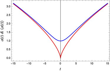
Figure 1: The behavior of $a(t)$ (red line) and $\langle a\rangle(T)$ (blue line) for $g_{s}(k)\neq 0$ in the gauge $N=1$, i.e., $T=t$. The bouncing behavior of the quantum mechanical solution is apparent at $t=0$.

III.2 Case $g_{r}\neq 0$

In this case, the classical equations of motion in the gauge $N=a(t)$ read

$$\dot{a} = -\frac{p_{a}}{6(3\lambda-1)},$$ (70)

$$\dot{p}_{a} = -\frac{{p_{a}}^{2}}{12(3\lambda-1)a}+\frac{g_{r}}{a},$$ (71)

$$\dot{T} = a(t).$$ (72)

After eliminating $p_{a}$ from Eqs. (70) and (71), we obtain

$$\ddot{a}-\frac{\dot{a}^{2}}{2a}+\frac{g_{r}}{6(3\lambda-1)a}=0.$$ (73)

Also, the constraint $\mathcal{H}=0$ leads to

$$\dot{a}^{2}=\frac{1}{3(3\lambda-1)}(g_{r}+p_{T}\,a).$$ (74)

For $\lambda\neq\frac{1}{3}$, the solution reads

$$a(t)=\alpha t^{2}+\beta t,$$ (75)

where $\alpha=\frac{p_{T}}{12(3\lambda-1)}$ and $\beta=\sqrt{\frac{g_{r}}{3(3\lambda-1)}}$.

For the quantum solution, the time-independent SWD equation reads

$$\frac{d^{2}\psi}{da^{2}}-12(3\lambda-1)E\left(a-\frac{g_{r}}{E}\right)\psi=0.$$ (76)

Using the variable $x=(12(3\lambda-1)E)^{\frac{1}{3}}\left(a-\frac{g_{r}}{E}\right)$, the above equation can be written as

$$\frac{d^{2}\psi}{dx^{2}}-x\psi=0,$$ (77)

and the solutions are the Airy functions:

$$\psi(x) = C_{1}\;\mathrm{Ai}(x)\;+\;C_{2}\;\mathrm{Bi}(x).$$ (78)

Airy functions $\mathrm{Ai}(x)$ [$\mathrm{Bi}(x)$] have oscillatory behaviors for $x<0$ ($a<\frac{g_{r}}{E}$) and decrease (increase) exponentially for $x>0$ ($a>\frac{g_{r}}{E}$) which shows that $\mathrm{Bi}(x)$ is physically unacceptable. Therefore, we find

$$\psi(a,T)=\mathrm{Ai}\left[(12(3\lambda-1)E)^{\frac{1}{3}}\left(a-\frac{g_{r}}{E}\right)\right].$$ (79)

Now, the DeWitt boundary condition implies

$$-\left(\frac{12(3\lambda-1)}{E_{n}^{2}}\right)^{\frac{1}{3}}g_{r}=r_{n},$$ (80)

where $r_{n}$ are zeros of the Airy function. Therefore, the energy spectrum reads

$$E_{n}=\pm\sqrt{12(3\lambda-1)}\left(-\frac{g_{r}}{r_{n}}\right)^{\frac{3}{2}},$$ (81)

and the time-dependent solutions take the form

$$\Psi_{n}(a,T)=e^{-iE_{n}T}\mathrm{Ai}\left[(12(3\lambda-1)E_{n})^{\frac{1}{3}}a+r_{n}\right].$$ (82)

Notice that, for $E>0$, the Airy’s function $\mathrm{Ai}(x)$ exhibits an oscillatory behavior for $x<0$ ($a<\frac{g_{r}}{E}$), whereas for $x>0$ ($a>\frac{g_{r}}{E}$), it decreases monotonically and for large $x$ becomes an exponentially damped function. Therefore, contrary to what is usually expected, Eq. (82) represents a classical behavior for small $a$ and a quantum behavior for large values of the scale factor. This is in contrast to the usual expected results. In fact, detecting quantum gravitational effects in large Universes is noticeable which is also observed in the FRW, Stephani, and Kaluza-Klein models in the context of general relativity Pedram 2007 ; Lemos ; Colistete . Note that for $E>0$, the solution (82) is squared integrable.

III.3 Case $g_{\Lambda}\neq 0$ and $g_{s}\neq 0$

In this case, the dynamics of the classical system in the gauge $N=1$ is governed by

$$\dot{a} = -\frac{p_{a}}{6(3\lambda-1)a},$$ (83)

$$\dot{p}_{a} = -\frac{{p_{a}}^{2}}{12(3\lambda-1)a^{2}}-3g_{\Lambda}a^{2}+\frac{3g_{s}}{a^{4}},$$ (84)

$$\dot{T} = 1.$$ (85)

So, we obtain

$$\ddot{a}+\frac{\dot{a}^{2}}{2a}+\frac{1}{2(3\lambda-1)}\left(-g_{\Lambda}a+\frac{g_{s}}{a^{5}}\right)=0.$$ (86)

Also, the constraint $\mathcal{H}=0$ leads to

$$\dot{a}^{2}=\frac{1}{3(3\lambda-1)}\left(g_{\Lambda}a^{2}+\frac{g_{s}}{a^{4}}+\frac{p_{T}}{a}\right).$$ (87)

For $\lambda\neq\frac{1}{3}$ and $g_{\Lambda}\neq 0$, the solution reads

$$a(t)=\left[\sqrt{\frac{g_{s}}{g_{\Lambda}}}\sinh\chi t+\frac{p_{T}}{2g_{\Lambda}}(\cosh\chi t-1)\right]^{\frac{1}{3}},$$ (88)

where $\chi=\sqrt{\frac{3g_{\Lambda}}{3\lambda-1}}$.

For the quantum solution, the time-independent SWD equation is

$$\frac{d^{2}\psi(a)}{da^{2}}+12(3\lambda-1)\Big{(}g_{\Lambda}(k)a^{4}-Ea$$

$$\qquad+\frac{g_{s}(k)}{a^{2}}\Big{)}\psi(a) = 0.$$ (89)

For $\lambda>\frac{1}{3}$ the solution is

$$\psi(a)=C_{1}\;\frac{1}{a}\;\mathrm{M}_{\mu,\nu}(\xi a^{3})\;+\;C_{2}\;\frac{1}{a}\;\mathrm{W}_{\mu,\nu}(\xi a^{3}),$$ (90)

where $\mathrm{M}_{\mu\nu}(x)$ and $\mathrm{W}_{\mu\nu}(x)$ are Whittaker functions upon choosing $\mu=iE\sqrt{\frac{3\lambda-1}{3g_{\Lambda}}}$, $\nu=\frac{1}{6}\sqrt{1-48(3\lambda-1)g_{s}}$, and $\xi=4i\sqrt{\frac{(3\lambda-1)g_{\Lambda}}{3}}$. Now the DeWitt boundary condition is fulfilled if we set $C_{1}\neq 0$ and $C_{2}=0$.

III.4 Case $g_{c}\neq 0$, $g_{s}\neq 0$, and $g_{r}\neq 0$

The time-independent SWD equation for this case reads

$$\frac{d^{2}\psi(a)}{da^{2}}+12(3\lambda-1)\Big{(}-g_{c}(k)a^{2}+g_{r}(k)$$

$$+\frac{g_{s}(k)}{a^{2}}-Ea\Big{)}\psi(a) = 0.$$ (91)

The solution for $\lambda>\frac{1}{3}$ is given by

$$\psi(a) = C_{1}\;e^{\kappa(g_{c}a^{2}+Ea)}a^{\frac{1+\alpha}{2}}\mathrm{B}_{\alpha,\beta,\gamma,\delta}(\xi a)$$ (92)

$$+\;C_{2}\;e^{\kappa(g_{c}a^{2}+Ea)}a^{\frac{1-\alpha}{2}}\;\mathrm{B}_{-\alpha,\beta,\gamma,\delta}(\xi a),$$

where $\mathrm{B}_{\alpha,\beta,\gamma,\delta}(x)$ is the biconfluent Heun function heun , and $\kappa=\sqrt{\frac{3(3\lambda-1)}{g_{c}}}$, $\alpha=\sqrt{1-48(3\lambda-1)g_{s}}$, $\beta=i\left(\frac{12(3\lambda-1)}{g_{c}^{3}}E\right)^{\frac{1}{4}}E$, $\gamma=-\sqrt{\frac{3(3\lambda-1)}{g_{c}^{3}}}\frac{4g_{r}g_{c}+E^{2}}{2g_{c}}$, $\delta=0$, and $\xi=i(12(3\lambda-1)g_{c})^{\frac{1}{4}}$. The above solution with $C_{1}\neq 0$ and $C_{2}\neq 0$ satisfies the DeWitt boundary condition for $0<g_{s}<\frac{1}{48(3\lambda-1)}$.

III.5 Case $g_{\Lambda}\neq 0$, $g_{c}\neq 0$, and $g_{r}\neq 0$

In this case, the time-independent SWD equation is

$$\frac{d^{2}\psi(a)}{da^{2}}+12(3\lambda-1)\Big{(}g_{\Lambda}a^{4}-g_{c}(k)a^{2}$$

$$+g_{r}(k)-Ea\Big{)}\psi(a) = 0,$$ (93)

and the solution for $\lambda>\frac{1}{3}$ reads

$$\psi(a) = C_{1}\;e^{\kappa(2g_{\Lambda}a^{3}-3g_{c}a)}\;\mathrm{T}_{\alpha,\beta,\gamma}(\xi a)$$ (94)

$$+\;C_{2}\;e^{-\kappa(2g_{\Lambda}a^{3}-3g_{c}a)}\;\mathrm{T}_{\alpha,-\beta,\gamma}(-\xi a),$$

where $\mathrm{T}_{\alpha,\beta,\gamma}(x)$ is the triconfluent Heun function heun , and $\kappa=\sqrt{-\frac{3\lambda-1}{3g_{\Lambda}}}$, $\alpha=\frac{3}{2}\frac{g_{c}^{2}-4g_{\Lambda}g_{r}}{g_{\Lambda}}\left(\frac{3(3\lambda-1)^{2}}{2g_{\Lambda}}\right)^{\frac{1}{4}}$, $\beta=-3E\sqrt{-\frac{3(3\lambda-1)}{g_{\Lambda}}}$, $\gamma=g_{c}\left(\frac{18(3\lambda-1)}{g_{\Lambda}^{2}}\right)^{\frac{1}{3}}$, and $\xi=\left(-\frac{16(3\lambda-1)g_{\Lambda}}{3}\right)^{\frac{1}{6}}$. Note that $\mathrm{T}_{\alpha,\beta,\gamma}(x)$ do not obey the DeWitt boundary condition.

III.6 Case $g_{c}(k)\neq 0$ and $g_{r}(k)\neq 0$

In the particular case $g_{\Lambda}(k)=0$ and $g_{s}(k)=0$, the classical dynamics of the system in gauge $N=a$ is governed by

$$\dot{a} = -\frac{p_{a}}{6(3\lambda-1)},$$ (95)

$$\dot{p}_{a} = -\frac{p_{a}^{2}}{12(3\lambda-1)a}+g_{c}(k)a+\frac{g_{r}(k)}{a}$$ (96)

$$\dot{T} = a(t),$$ (97)

so, we have

$$\ddot{a}-\frac{\dot{a}^{2}}{2a}+\frac{1}{6(3\lambda-1)}\left(g_{c}(k)a+\frac{g_{r}(k)}{a}\right)=0.$$ (98)

Also, using the Hamiltonian’s constraint $\mathcal{H}=0$, we find

$$\dot{a}^{2}+\frac{a}{3(3\lambda-1)}\left(g_{c}(k)\,a-\frac{g_{r}(k)}{a}-p_{T}\right)=0.$$ (99)

Thus, the classical solution reads

$$a(t)=\sqrt{\frac{g_{r}}{g_{c}}}\sin\omega t+\frac{p_{T}}{2g_{c}}\left(1-\cos\omega t\right),$$ (100)

where $\omega=\sqrt{\frac{g_{c}}{3(3\lambda-1)}}$ is the frequency of the oscillation.

At the quantum domain, the SWD equation is

$$\frac{d^{2}\psi}{da^{2}}+12(3\lambda-1)\left(g_{r}(k)-Ea-g_{c}(k)a^{2}\right)\psi=0,$$ (101)

where its solution reads

$$\psi_{n}(a)=e^{-\xi(a+E_{n}/2g_{c})^{2}}\;\mathrm{H}_{n}\left(\sqrt{2\xi}(a+E_{n}/2g_{c})\right).$$ (102)

Here, $\mathrm{H}_{n}(x)$ are Hermite functions, $\xi=\sqrt{3(3\lambda-1)g_{c}}$, and

$$E_{n}=\pm 2g_{c}\sqrt{\frac{2n+1}{2\xi}-\frac{g_{r}}{g_{c}}}\,,\qquad n=0,1,2,\ldots\,.$$ (103)

Therefore, the time-dependent squared integrable solution is

$$\Psi_{n}(a,T) = N_{n}\,e^{-iE_{n}T}\psi_{n}(a)$$ (104)

$$= N_{n}\,e^{-iE_{n}T}e^{-\xi\left(a+E_{n}/2g_{c}\right)^{2}}$$

$$\quad\times\mathrm{H}_{n}\left(\sqrt{2\xi}(a+E_{n}/2g_{c})\right),$$

where

$$N_{n}=\sqrt{\frac{-\xi}{2^{n-1}n!{\sqrt{\pi}d_{n}}}}$$ (105)

is the normalization coefficient and $d_{n}=\frac{E_{n}}{2g_{c}}\sqrt{2\xi}$. The eigenfunctions (104) do not satisfy either of the two boundary conditions (47) and (48). Indeed, $\Psi_{n}(a,T)$ is similar to the stationary quantum wormholes which is defined by Hawking. However, this model does not represent static quantum wormholes which are ruled out by the requirement of the self-adjointness of the Hamiltonian AFLM .

Now, assuming the minus sign in Eq. (103) due to the condition $N_{n}^{2}>0$ and taking $\lambda>\frac{1}{3}$, $g_{c}\neq 0$, and $g_{r}<\frac{g_{c}}{2\xi}$, we construct wave packets upon superimposing the above eigenfunctions (104):

$$\Psi(a,T)=\sum_{n=0}^{\infty}A_{n}\Psi_{n}(a,T).$$ (106)

Using the initial wave function,

$$\Psi(a,T=0)\,=\,2\sqrt{2}\,\xi\,a\,e^{-\xi a^{2}},$$ (107)

the expansion coefficients are given by

$$A_{n} = \frac{N_{n}}{\sqrt{\xi}}\int_{-\infty}^{\infty}dx\,x^{2}\,e^{-\frac{x^{2}}{2}}e^{\frac{(x+d_{n})^{2}}{2}}\mathrm{H}_{n}(x+d_{n}),$$ (108)

$$= \frac{N_{n}}{4}\sqrt{\frac{\pi}{\xi}}\,e^{-{{d_{n}}^{2}}/4}\,(d_{0}\,d_{1})^{2}{d_{n}}^{n-2}.$$

Thus, the time evolution of the expectation value of the scale factor, namely,

$$\langle a\rangle(T)=\frac{\int_{0}^{\infty}da\;a^{2}\;\Psi^{\ast}(a,T)\Psi(a,T)}{\int_{0}^{\infty}da\;a\;\Psi^{\ast}(a,T)\Psi(a,T)},$$ (109)

can be consequently obtained. Note that, the relation between $T$ and the cosmic time $t$ is given by

$$T=\frac{1}{\omega}\sqrt{\frac{g_{r}}{g_{c}}}(1-\cos\omega t)+\frac{p_{T}}{2g_{c}}\left(t-\frac{\sin\omega t}{\omega}\right).$$ (110)

Figure 2 shows the behavior of $\langle a\rangle(t)$ for $\lambda=1$, $g_{c}=2$, $g_{r}=0.1$, and $p_{T}=2g_{c}$. As the figure shows, $\langle a\rangle(t)$ exhibits an oscillatory and nonvanishing behavior. This would be a sign that the model is singularity free in the quantum domain.

Note that although the eigenfunctions (104) do not satisfy either of the two boundary conditions (47), (48), using the initial wave function (107), the expectation value of the scale factor never tends to the singular point. This shows that the evolution of the Universe is uniquely determined by the initial wave packet, and no boundary condition at $a=0$ is necessary. A similar behavior is also observed for the perfect fluid HL quantum cosmology HL . The oscillatory behavior of the solution also appears in other quantum cosmological models Monerat .

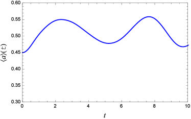
Figure 2: The evolution of the expectation value of the scale factor (109) with respect to the cosmic time $t$. We set $\lambda=1$, $g_{c}=2$, $g_{r}=0.1$, and $p_{T}=2g_{c}$.

IV Conclusions

In this work, we have studied the Hořava-Lifshitz quantum cosmology in the presence of the Chaplygin gas and in the framework of the Schutz formalism. Due to the asymmetry of space and time in the HL gravity, the ADM decomposition would be a natural scheme to obtain the Hamiltonian of the model. On the other hand, the Chaplygin gas model could describe a transition from a Universe filled with dustlike matter to an accelerating expanding stage. As a poor approximation the present approach reduces the brane physics into Hořava-Lifshitz gravity plus the generalized Chaplygin gas. Although the HL gravity is not fully compatible with general relativity, we showed that a period of inflation can be achieved. In particular, the nonprojectable Hořava-Lifshitz gravity is equivalent to the Einstein-ether theory with a hypersurface orthogonal ether at low energy Soti .

Using Schutz variational formalism, we obtained the SWD equation where the matter degrees of freedom played the role of time. We exactly solved the SWD equation for various cases. For two cases, namely, $g_{s}(k)\neq 0$ (Sec. III.1) and $g_{c}(k)\neq 0$ and $g_{r}(k)\neq 0$ (Sec. III.6), we constructed wave packets upon choosing appropriate initial conditions. In both cases, unlike the classical solutions, the expectation value of the scale factor avoids the singularity in the quantum domain. For $g_{s}(k)\neq 0$ the wave function of the Universe is given by the Bessel functions with order $\nu=\frac{1}{3}\sqrt{1-48(3\lambda-1)g_{s}}$, whereas the order of the Bessel functions is $\nu=1/3$ for the Chaplygin gas FRW quantum cosmology with zero spatial curvature ($k=0$) in the context of general relativity. In Sec. III.1, we constructed a wave packet that agrees with the classical solution at late times. It is worth mentioning that, for this case, the notion of time that arises from Schutz formalism coincides with the cosmological time at late times.

In Sec. III.2, we found classical behavior for small values of the scale factor and a quantum behavior for its large values. This unexpected result is also observed in the FRW, Stephani, and Kaluza-Klein models in the context of general relativity. The bouncing behavior of the expectation value of the scale factor could be related to the existence of a minimal length scale $\langle a\rangle_{\mathrm{min}}=\left[\frac{\Gamma\left(\nu+\frac{4}{3}\right)}{\Gamma(\nu+1)}\right]^{2}\left(\frac{16(3\lambda-1)p_{T}}{3}\right)^{-\frac{1}{3}}$ which is suggested by various proposals of quantum gravity. In Sec. III.6, we found that the evolution of the wave function of the Universe is uniquely determined by the initial wave packet, i.e., no boundary condition at $a=0$ is necessary in HL quantum cosmology.

Among various presented solutions, solutions (75), i.e., $a(t)=\alpha t^{2}+\beta t$ and (88), i.e., $a(t)=\left[\sqrt{\frac{g_{s}}{g_{\Lambda}}}\sinh\chi t+\frac{p_{T}}{2g_{\Lambda}}(\cosh\chi t-1)\right]^{\frac{1}{3}}$ which show the accelerated expansion of the Universe, namely, $\ddot{a}>0$, could match the inflation scenario. In particular, solution (75) tends to the power-law inflation $a(t)\propto\alpha t^{2}$ and solution (88) tends to the exponential inflation $a(t)\propto\exp(\chi t/3)$. Observational data of the cosmic microwave background strongly indicate that the primordial cosmological perturbations have an almost scale-invariant spectrum. In general relativity ($z=1$), the scale invariance also requires inflation. Indeed, for this case, the scale invariance is nothing but the constancy of the Hubble expansion rate $H=\dot{a}/a$ which leads to $a\propto\exp(Ht)$. For general $z$, the amplitude of quantum fluctuations of the scalar field in HL gravity reads Muko

$$\delta\phi\sim M\times\left(\frac{H}{M}\right)^{\frac{3-z}{2z}},$$ (111)

where $M$ is some energy scale. For $z=3$ it is reduced to $\delta\phi\sim M$, which means that the amplitude of quantum fluctuations does not depend on the Hubble expansion rate. In other words, the spectrum of cosmological perturbations in Hořava-Lifshitz gravity with $z=3$ is automatically scale invariant even without inflation. In fact, the power law expansion $a\propto t^{p}$ with $p>1/z$ satisfies the condition. In our study, solutions (60), (75), and (88) satisfy this condition. Notice that although solution (60), i.e., $a(t)=(\alpha t^{2}+\beta t)^{\frac{1}{3}}$, is not an accelerating solution, it results in the scale-invariant spectrum in HL gravity.

- (1) Supernova Search Team Collaboration, A. G. Riess et al., Astron. J. 116, 1009 (1998).
- (2) Supernova Cosmology Project Collaboration, S. Perlmutter et al., Astrophys. J. 517, 565 (1999).
- (3) J. L. Tonry et al., Astrophys. J. 594, 1 (2003).
- (4) D. N. Spergel et al., Astrophys. J. Suppl. 148, 175 (2003).
- (5) C. L. Bennett et al., Astrophys. J. Suppl. 148, 1 (2003).
- (6) SDSS Collaboration, M. Tegmark et al., Phys. Rev. D 69, 103501 (2004).
- (7) S. Weinberg, Rev. Mod. Phys. 61, 1 (1989).
- (8) P. J. E. Peebles and B. Ratra, Rev. Mod. Phys. 75, 559 (2003).
- (9) M. C. Bento, O. Bertolami, and A. A. Sen, Phys. Rev. D 66, 043507 (2002).
- (10) H. B. Benaoum, Adv. High Energy Phys. 2012, 357802 (2012).
- (11) H. Saadat and B. Pourhassan, Int. J. Theor. Phys. 53, 1168 (2014).
- (12) X-H. Zhai, Y-D. Xu, and X-Z. Li, Int. J. Mod. Phys. D 15, 1151 (2006).
- (13) A. Y. Kamenshchik, U. Moschella, and V. Pasquier, Phys. Lett. B 511, 265 (2001).
- (14) N. Bilic, G. B. Tupper, and R. D. Viollier, Phys. Lett. B 535, 17 (2002).
- (15) U. Debnath, A. Banerjee, and S. Chakraborty, Classical Quantum Gravity 21, 5609 (2004).
- (16) H. Saadat and B. Pourhassan, Astrophys. Space Sci. 344, 237 (2013).
- (17) J. Naji, B. Pourhassan, and A.R. Amani, Int. J. Mod. Phys. D 23, 1450020 (2013).
- (18) B. Pourhassan, Int. J. Mod. Phys. D 22, 1350061 (2013).
- (19) J. Sadeghi, B. Pourhassan, M. Khurshudyan, and H. Farahani, Int. J. Theor. Phys. 53, 911 (2014).
- (20) M. Bouhmadi-Lopez and P. V. Moniz, Phys. Rev. D 71, 063521 (2005); AIP Conf. Proc. 736, 188 (2004).
- (21) O. Bertolami and V. Duvvuri, Phys. Lett. B 640, 121 (2006).
- (22) M. Bouhmadi-Lopez, C. Kiefer, B. Sandhofer, and P.V. Moniz, Phys. Rev. D 79, 124035 (2009).
- (23) M. Bouhmadi-Lopez, P. Frazao, and A. B. Henriques, Phys. Rev. D 81, 063504 (2010); arXiv:1002.4785.
- (24) M. Bouhmadi-Lopez, P. Chen, and Y.-W. Liu, Phys. Rev. D 84, 023505 (2011); AIP Conf. Proc. 1458, 327 (2012).
- (25) M. Bouhmadi-Lopez, J. Morais, and A. B. Henriques, Phys. Rev. D 87, 103528 (2013).
- (26) R. Jackiw, arXiv:physics/0010042; N. Ogawa, Phys. Rev. D 62, 085023 (2000); A. Kamenshchik, U. Moschella, and V. Pasquier, Phys. Lett. B 487, 7 (2000); J.C. Fabris, S.V.B. Goncalves, and P.E. de Souza, Gen. Relativ. Gravit. 34, 53 (2002).
- (27) S. del Campo and R. Herrera, Phys. Lett. B 660, 282 (2008).
- (28) P. Vargas Moniz, Classical Quantum Gravity 19, L127 (2002); Phys. Rev. D 66, 064012 (2002); Phys. Rev. D 66, 103501 (2002); H. Q. Lu, T. Harko, and K. S. Cheng, Int. J. Mod. Phys. D 8, 625 (1999).
- (29) M. Bouhmadi-Lopez and J. A. Jimenez Madrid, J. Cosmol. Astropart. Phys. 05 (2005) 005; J.-G. Hou and X.-Z. Li, Phys. Lett. B 606, 7 (2005); S. Srivastava, Phys. Lett. B 619, 1 (2005).
- (30) N. Arkani-Hamed, S. Dimopoulos, and G. R. Dvali, Phys. Lett. B 429, 263 (1998).
- (31) J. Khoury, B.A. Ovrut, P. J. Steinhardt, and N. Turok, Phys. Rev. D 64, 123522 (2001).
- (32) A. Davidson, D. Karasik, and Y. Lederer, Classical Quantum Gravity 16, 1349 (1999); A. Davidson and D. Karasik, Mod. Phys. Lett. A 13, 2187 (1998); A. Davidson, Classical Quantum Gravity 16, 653 (1999).
- (33) J. Garriga and M. Sasaki, Phys. Rev. D 62, 043523 (2000); M. Bouhmadi and P. F. Gonzalez-Dyaz, Phys. Rev. D 65, 063510 (2002); M. Bouhmadi-Lopez, P. F. Gonzalez-Dyaz, and A. Zhuk, Classical Quantum Gravity 19, 4863 (2002).
- (34) K. Koyama and J. Soda, Phys. Lett. B 483, 432 (2000).
- (35) L. Anchordoqui, C. Nunez, and K. Olsen, J. High Energy Phys. 10 (2000) 050.
- (36) S. Nojiri and S. D. Odintsov, J. Cosmol. Astropart. Phys. 06 (2003) 004.
- (37) S. S. Seahra, H. R. Sepangi, and J. Ponce de Leon, Phys. Rev. D 68, 066009 (2003).
- (38) A. Sanyal, arXiv:0305042.
- (39) S. del Campo, J. Cosmol. Astropart. Phys. 11 (2013) 004.
- (40) T. Barreiro, O. Bertolami, and P. Torres, Phys. Rev. D 78, 043530 (2008).
- (41) Since our study is in the preinflationary phase, the current bounds on the GCG parameters are not relevant for the preinflationary phase.
- (42) M. Bouhmadi-Lopez, Pisin Chen, Y.-C Huang, and Y.-H Lin, Phys. Rev. D 87, 103513 (2013).
- (43) C. Kiefer and H. D. Zeh, Phys. Rev. D 51, 4145 (1995).
- (44) D. Giulini, E. Joos, C. Kiefer, J. Kupasch, I.-O. Stamatescu, and H. D. Zeh, Decoherence and the Appearance of a Classical World in Quantum Theory (Spinger-Verlag, Berlin, 1996).
- (45) C. Kiefer, Quantum Gravity (Oxford University Press, New York, 2004).
- (46) L. Diosi and C. Kiefer, Phys. Rev. Lett. 85, 3552 (2000).
- (47) B. F. Schutz, Phys. Rev. D 2, 2762 (1970).
- (48) B. F. Schutz, Phys. Rev. D 4, 3559 (1971).
- (49) E. Gourgoulhon, arXiv:gr-qc/0703035.
- (50) P. Horava, J. High Energy Phys. 03 (2009) 020.
- (51) P. Horava, Phys. Rev. D 79, 084008 (2009).
- (52) P. Horava, Phys. Rev. Lett. 102, 161301 (2009).
- (53) P. Horava, Phys. Lett. B 694, 172 (2010).
- (54) O. Obregon and J. A. Preciado, Phys. Rev. D 86, 063502 (2012).
- (55) D. Blas, O. Pujolas, and S. Sibiryakov, J. High Energy Phys. 04 (2011) 018.
- (56) T. P. Sotiriou, M. Visser, and S. Weinfurtner, J. High Energy Phys. 10 (2009) 033.
- (57) J. Bellorin and A. Restuccia, Phys. Rev. D 84, 104037 (2011).
- (58) A. Wang and R Maartens, Phys. Rev. D 81, 024009 (2010).
- (59) S. Carloni, E. Elizalde, and P. J. Silva, Classical Quantum Gravity 27, 045004 (2010).
- (60) S. Carloni, E. Elizalde, and P. J. Silva, Classical Quantum Gravity 28, 195002 (2011).
- (61) T. Zhu, F. -W. Shu, Q. Wu, and A. Wang, Phys. Rev. D 85, 044053 (2012).
- (62) T. P. Sotiriou, M. Visser, and S. Weinfurtner, Phys. Rev. Lett 102, 251601 (2009).
- (63) B. Vakili and V. Kord, Gen. Rel. Grav. 45 1313 (2013).
- (64) J. P. M. Pitelli and A. Saa, Phys. Rev. D 86, 063506 (2012).
- (65) T. M. Helliwell and D. A. Konkowski, V. Arndt, Gen. Relativ. Gravit. 35, 79 (2003).
- (66) A. Ali, S. Dutta, E. N. Saridakis, and A. A. Sen, Gen. Relativ. Gravit. 44, 657 (2012).
- (67) B. Pourhassan, arXiv:1412.2605.
- (68) B. C. Paul, P. Thakur, Pramana 81, 691 (2013).
- (69) O. Bertolami and C.A.D. Zarro, Phys. Rev. D 84, 044042 (2011).
- (70) S. Mukohyama, Classical Quantum Gravity 27, 223101 (2010).
- (71) T.P. Sotiriou, J. Phys. Conf. Ser. 283, 012034 (2011).
- (72) V. G. Lapchinskii and V. A. Rubakov, Theor. Math. Phys. 33, 1076 (1977).
- (73) P. Pedram, S. Jalalzadeh, and S. S. Gousheh, Int. J. Theor. Phys. 46, 3201 (2007).
- (74) P. Pedram and S. Jalalzadeh, Phys. Lett. B 659, 6 (2008).
- (75) E. Elizalde and P. J. Silva, J. High Energy Phys. 06 (2012) 049.
- (76) P. Pedram, S. Jalalzadeh, and S.S. Gousheh, Classical Quantum Gravity 24, (2007).
- (77) N.A. Lemos and F.G. Alvarenga, Gen. Relativ. Gravit. 31, 1743 (1999).
- (78) R. Colistete Jr., J.C. Fabris, and N. Pinto-Neto, Phys. Rev. D 57, 4707 (1998).
- (79) A. M. Ishkhanyan, arXiv:1412.0654.
- (80) F. G. Alvarenga, J. C. Fabris, N. A. Lemos, and G. A. Monerat, Gen. Relativ. Gravit. 34, 651 (2002).
- (81) G.A. Monerat, E.V.C. Silva, G. Oliveira-Neto, L.G.F. Filho, and N.A. Lemos, Phys. Rev. D 73, 044022 (2006).