Weak values obtained from mass-energy equivalence

Abstract

Quantum weak measurement, measuring some observable quantities within the selected subensemble of the entire quantum ensemble, can produce many interesting results such as the superluminal phenomena. An outcome of such a measurement is the weak value which has been applied to amplify some weak signals of quantum interactions in lots of previous references. Here, we apply the weak measurement to the system of relativistic cold atoms. According to mass-energy equivalence, the internal energy of an atom will contribute its rest mass and consequently the external momentum of center of mass. This implies a weak coupling between the internal and external degrees of freedom of atoms moving in the free space. After a duration of this coupling, a weak value can be obtained by post-selecting an internal state of atoms. We show that, the weak value can change the momentum uncertainty of atoms and consequently help us to experimentally measure the weak effects arising from mass-energy equivalence.

I Introduction

Almost 30 years ago, Aharonov, Albert, and Vaidman introduced the theory of quantum weak measurement AAV . This measurement has a key feature: after a weak coupling between the quantum systems, the relevant observable quantities are measured in some post-selected subensembles. An outcome of weak measurements is the so-called weak value, $A_{w}$, which is a complex number and depends on the post-selected state Jozsa ; imaginary ; Anomalous . Physically, the pure state of a quantum system will be destroyed by the postselection and then becomes a mixed state which is constituted by two pure states. Selecting out one of the pure states to be measured, some new phenomena appear because the selected wave function is very different from the original one (before the postselection). The postselection is actually a physical operation applied on the quantum state, so that the weak measurement can be regarded as a quantum coherent operation plus a classical selection (filtering). Hence, the weak measurement is indeed different from the usual measurement in physics.

Recently, in refs. Nature-wavefuction ; Science-trajectory ; HD ; LG ; Hall Effect ; CatNJPA ; Cat ; CatNJP ; SuperluminalPTL ; SuperluminalCherenkov ; SuperluminalBeryy ; SuperluminalSteinberg ; Electrons , novel phenomena within the weak measurements were reported, such as the spin Hall effect of light Hall Effect , the Cheshire cat CatNJPA ; Cat ; CatNJP , and the superluminal phenomena SuperluminalPTL ; SuperluminalCherenkov ; SuperluminalBeryy ; SuperluminalSteinberg . Remarkably, lots of studies have shown that the weak measurements can be utilized to implement signal amplifications Amplification0 ; Amplification1 ; Amplification2 ; Amplification3 ; Amplification4 ; Amplification5 ; Amplification6 ; AB ; arXiv . Most of these references use a laser to realize the desired weak measurements RMP . The necessary quantum interaction for weak value gain was realized via the crystal-induced coupling between the polarization and momentum of lights. Similar to the lights, the matter wave should be also applicable for realizing the desired weak measurements. Recently, this was demonstrated in neutron interferometry neutron . In such an experiment, an external magnetic field was applied to generate the spin-orbit coupling of neutron, and the weak value was obtained by post-selecting a spin state.

Here, we propose using weak value to test mass-energy equivalence in the system of coherent atoms. Usually, the mass $m$ in the Schrödinger or Dirac equation is treated as a constant quality. However, the mass-energy equivalence says that the internal energy of a particle will contribute its rest mass E=mc2 . Hence, the quality $m$ is no longer a constant but depends on the particle’s internal energies. This implies a weak coupling between the internal and external degrees of freedom of particles Zych1 ; Zych2 ; Pikovski ; arXivDennis ; Pollock . The potential coupling cannot be explained by the usual notation of time-dilation Hafele-Keating ; Zhu2010 ; Mueller ; 1993 because the rest-mass is now regarded as a quantum mechanics operator (for the internal superposition states). A recent interesting article Pikovski showed that the coupling due to the mass-energy equivalence is perhaps an universal decoherence for quantum systems in the gravitational field. As mentioned in Ref. Zych1 , measuring the possible dynamic coupling induced by mass-energy equivalence is still a challenge in experiments due to its very weak interacting strength. Here, we design a weak measurement setup for observing the predicted effects of mass-energy equivalence. We consider a two-level atom whose internal qubit and external center-of-mass (c.m.) motion are coupled naturally due to the mass-energy equivalence. Based on this coupling, the weak value is obtained by post-selecting the atomic internal state. We show that the present weak value could offer some certain advantages for experimentally detecting the ultraweak coupling induced by mass-energy equivalence.

This article is organized as follows. In Sec. II, we briefly review the basic principles and the usefulness of quantum weak measurements. In Sec. III, we analyze the mass-energy-equivalence-induced coupling between the internal and external degrees of freedom of a two-level atom. Based on this coupling, the complex weak value is obtained by post-selecting a proper internal state of atom. Considering the practical atomic system is in an earth-based laboratory, the gravitational effect is also studied. In Sec. IV, we use the atomic Kapitza-Dirac (KD) scattering to prepare the coherent atoms with large momentum uncertainty atomoptics . Such a light-induced scattering of atoms is further utilized to realize the desired postselection of atomic internal states. Finally, we present our conclusions in Sec. V.

II The basic principles for quantum weak measurements

Consider two interacting quantum systems, namely Alice and Bob, with the coupling Hamiltonian $\hat{H}=\hbar g_{0}\hat{A}\hat{B}$. Here, $\hbar$ is the Planck constant divided by $2\pi$. $\hat{A}$ and $\hat{B}$ are the operators that change respectively Alice and Bob’s states. The coupling strength between the two quantum systems is $g_{0}$. After an interaction of duration $t$, the final state of the total system can be approximately written as

$$|\psi\rangle=e^{\frac{-i\hat{H}t}{\hbar}}|A_{i}\rangle|B_{i}\rangle\approx|A_{i}\rangle|B_{i}\rangle-ig\hat{A}\hat{B}|A_{i}\rangle|B_{i}\rangle\,$$ (1)

under the weak interaction limit $g=g_{0}t\rightarrow 0$. Here, $|A_{i}\rangle$ and $|B_{i}\rangle$ are respectively the initial states of Alice and Bob, and the high orders of $g$ have been neglected. Considering Alice as a two-level system and then using its two orthonormal states $|A_{s}\rangle$ and $|A_{d}\rangle$, the state (1) can be expanded by

$$|\psi\rangle=(\langle A_{s}|A_{i}\rangle)|A_{s}\rangle|B_{s}\rangle+(\langle A_{d}|A_{i}\rangle)|A_{d}\rangle|B_{d}\rangle$$ (2)

with the unnormalized wave functions $|B_{s}\rangle\approx(1-igA_{w}\hat{B})|B_{i}\rangle$ and $|B_{d}\rangle\approx(1-igA^{w}\hat{B})|B_{i}\rangle$. Here, $A_{w}=\langle A_{s}|\hat{A}|A_{i}\rangle/\langle A_{s}|A_{i}\rangle$ and $A^{w}=\langle A_{d}|\hat{A}|A_{i}\rangle/\langle A_{d}|A_{i}\rangle$ are the weak values. Numerically, when $\langle A_{s}|A_{i}\rangle\rightarrow 0$, we have $|A_{w}|\rightarrow\infty$ and $|A^{w}|\rightarrow\langle A_{i}|\hat{A}|A_{i}\rangle$.

In weak measurement, the observable qualities of Bob are measured in the post-selected subensemble of Alice’s state $|A_{s}\rangle$, and the relevant results are given by the following equation

$$\langle\hat{M}\rangle=\frac{\langle B_{s}|\hat{M}|B_{s}\rangle}{\langle B_{s}|B_{s}\rangle}\approx\langle B_{i}|\hat{M}|B_{i}\rangle+2g\text{Im}\left(A_{w}M_{B}\right)\,,$$ (3)

with

$$M_{B}=\langle B_{i}|\hat{M}\hat{B}|B_{i}\rangle-\langle B_{i}|\hat{M}|B_{i}\rangle\langle B_{i}|\hat{B}|B_{i}\rangle\,\,.$$ (4)

Above, $\hat{M}$ is a Hermitian operator of Bob. It can be seen that the $g$-induced effect is proportional to the imaginary part of $A_{w}M_{B}$. This indicates that the weak value can amplify the $g$-effect, significantly, with $|A_{w}|\rightarrow\infty$. It can be also found that, the Eq. (3) with $A_{w}=\langle A_{i}|\hat{A}|A_{i}\rangle$ just describes the usual results without the postselection. On quantum weak measurements, it is worth emphasizing the following two points:

(i) The result $\langle\hat{M}\rangle$ is obtained in the post-selected subensemble, it is not the conjoint-measurement $\hat{P}=\hat{M}|A_{s}\rangle\langle A_{s}|$ performed in the entire ensemble, i.e., $\langle\hat{M}\rangle\neq\langle\psi|\hat{P}|\psi\rangle$.

(ii) The observable quality $\hat{M}$ can be generalized to be $\hat{M}^{\prime}=\hat{U}_{2}^{\dagger}\hat{M}\hat{U}_{2}$. That is, one can perform any further operations, namely $\hat{U}_{2}$, on the selected state $|B_{s}\rangle$ and then measure the observable quality $\hat{M}$. The final result is $\langle B_{s}|\hat{U}_{2}^{\dagger}\hat{M}\hat{U}_{2}|B_{s}\rangle/\langle B_{s}|B_{s}\rangle$.

The only drawback of weak-value amplification is that the probability $P_{s}\approx|\langle A_{s}|A_{i}\rangle|^{2}$ for successfully post-selecting $|A_{s}\rangle$ decreased with the increasing of $|A_{w}|$. Hence, the weak-value amplification is applicable just for the quantum system which includes large numbers of microscopic particles. Serval recent papers show weak-value amplification offering no fundamental metrological advantage due to the necessarily reduced probability of successful postselection SSNR ; Fisher1 ; Fisher2 . Aiming at the practical experimental systems, some studies show that the weak measurement can still improve the precision of parameter estimation due to the detector saturation Jordan1 or some other systematic errors Zhu . Alternatively, the advantage of weak-value amplification can be simply explained by the following equation:

$$I=NP_{s}\langle\hat{M}\rangle+NP_{s}E_{\rm system}+E_{\rm random}\,\,.$$ (5)

Here, $I$ is the experimental signal of observable quality $\langle\hat{M}\rangle$. This signal is proportional to the number $NP_{s}$ of successfully post-selected particles (with $N$ being the total number of prepared particles). In practical experiments, the system error $NP_{s}E_{\rm system}$ and the random error $E_{\rm random}$ will both contribute to the outcome $I$ Miao . Certainly, the random error $E_{\rm random}$ can be overcome by increasing the number of particles, i.e., $NP_{s}\langle\hat{M}\rangle\gg E_{\rm random}$. However, the system error cannot be eliminated by increasing the particles input as it is proportional to $NP_{s}$. Hence, the weak value amplification, i.e., $\langle\hat{M}\rangle\gg E_{\rm system}$, could be useful for suppressing the system errors (when the random errors are negligible).

As pointed out in the previous references, e.g.,Ref. imaginary , the imaginary part $A_{w}^{i}$ of the weak value could be more useful than its real part $A_{w}^{r}$. It can be also seen from Eq. (3), when $M_{B}=\text{Re}$, that the standard measurement (with $A_{w}=\langle A_{i}|\hat{A}|A_{i}\rangle=\text{Re}$) does not work for measuring the parameter $g$. This implies that the imaginary weak values could reveal some new effects of $g$. In the following sections, we show that the imaginary weak value can change the momentum uncertainty of an atom moving in the free space.

III The mass-energy-equivalence-induced weak values

III.1 The dynamic evolution of a falling atom

We consider only two internal states of an atom, namely, the ground state $|g\rangle$ and the excited state $|e\rangle$. The ground and excited states describe the different internal energies, i.e., $E_{g}$ and $E_{e}=E_{g}+\hbar\omega$, respectively. Here, $\omega$ is the transition frequency between the two internal levels. According to mass-energy equivalence, the atom has different rest mass for $|g\rangle$ and $|e\rangle$, i.e., $m_{g}=E_{g}/c^{2}$ and $m_{e}=m_{g}+\hbar\omega/c^{2}$, with $c$ being the speed of light in vacuum. Together with the external c.m. motion, the total-energy of the atom can be expressed as

$$H =\sqrt{c^{2}p^{2}+(m_{g}+m_{c})^{2}c^{4}}$$ (6)

$$\approx(m_{g}+m_{c})c^{2}+\frac{p^{2}}{2(m_{g}+m_{c})}$$

$$\approx m_{g}c^{2}+\frac{p^{2}}{2m_{g}}+m_{c}(c^{2}-\frac{p^{2}}{2m_{g}^{2}})\,,$$

with $m_{c}=0$ (for the ground state) or $m_{c}=\hbar\omega/c^{2}$ (for the excited state). Here, $H$ is a classical Hamiltonian, $p^{2}=p_{x}^{2}+p_{y}^{2}+p_{z}^{2}$ is the vector product of three dimensional momentum, and the terms relating to the high orders of $p^{2}/(m_{g}c+m_{c}c)^{2}$ and $m_{c}/m_{g}$ have been neglected for simplification Zych2 .

In quantum mechanics, the atom is described by a coherent superposition of the two internal states, i.e., $|A_{i}\rangle=\alpha|g\rangle+\beta|e\rangle$, with the probability-amplitudes $\alpha$ and $\beta$. Thus, the internal-state-dependent Hamiltonian should be the following operator,

$$\hat{H}=(m_{g}c^{2}+\frac{\hat{p}^{2}}{2m_{g}})\hat{1}+\hbar\omega[1-\frac{\hat{p}^{2}}{2(m_{g}c)^{2}}]|e\rangle\langle e|\,,$$ (7)

with $\hat{1}=|g\rangle\langle g|+|e\rangle\langle e|$ and $\hat{p}^{2}=\hat{p}_{x}^{2}+\hat{p}_{y}^{2}+\hat{p}_{z}^{2}$. Therefore, the results of measurements $\langle g|\hat{H}|g\rangle$ and $\langle e|\hat{H}|e\rangle$ can satisfy the classical ones of Eq. (6). By neglecting the term $m_{g}c^{2}\hat{1}$ (which does not generate any effects in the present work), the Hamiltonian (7) reduces to

$$\hat{H}=\hbar\omega|e\rangle\langle e|+\left(1-\frac{\hbar\omega|e\rangle\langle e|}{mc^{2}}\right)\frac{\hat{p}^{2}}{2m}\,.$$ (8)

Here, we denote $m_{g}$ by $m$ for short (as it is frequently used in what follows). Obviously, the coupling $|e\rangle\langle e|\hat{p}^{2}$ induced by mass-energy equivalence depends basically on the parameter

$$g_{0}=\frac{\hbar\omega}{mc^{2}}\,,$$ (9)

i.e., a ratio between the energy of a photon and the rest energy of an atom (in the ground state). Such a ratio is very small, so the relevant interactions are negligible in the usual systems. For example, $g_{0}\approx 8\times 10^{-12}$ for the calcium atom, with mass $m\approx 6.7\times 10^{-26}$ Kg and the selected optical transition frequency $\omega\approx 4.6\times 10^{14}$ Hz. In the following, we suggest using the weak value to measure such an ultrasmall parameter.

Note that the gravity effect of neutral atoms is significant in the earth-based laboratory. Therefore, the above Hamiltonian should be generalized to be

$$\hat{H}=\hbar\omega|e\rangle\langle e|+\left(1-g_{0}|e\rangle\langle e|\right)\frac{\hat{p}^{2}}{2m}+\left(1+g_{0}|e\rangle\langle e|\right)m\bar{g}\hat{z}\,.$$ (10)

Here, the last term is due to the gravitational potential of the atom, and $\bar{g}$ is the magnitude of gravitational acceleration on earth. The coupling of $|e\rangle\langle e|\hat{z}$ is due to the so-called Einstein’s weak equivalence principle, i.e., the internal energy $\hbar\omega$ will also contribute the gravitational potentials to atom. In fact, the Hamiltonian (10) describes a falling object with the different rest-masses which are internal-state dependent. The different rest masses (or say the different objects) will lead to the different diffraction patterns in the process of falling 1997 ; 2004 . Some more detailed studies on gravity-induced coupling can be seen in Refs. Zych1 ; Zych2 ; Pikovski ; arXivDennis . In this work, we do not measure the gravity effects. However, the relevant studies on Hamiltonian (10) are necessary, because our suggested measurements for coupling $|e\rangle\langle e|\hat{p}^{2}$ are implemented in the earth-based laboratory.

In terms of $g_{0}$ couplings, we rewrite Hamiltonian (10) as

$$\hat{H}=\hat{H}_{0}-g_{0}\hat{H}_{rc}-g_{0}\hat{H}_{zc}\,,$$ (11)

with a decoupled Hamiltonian

$$\hat{H}_{0}=\hbar\omega|e\rangle\langle e|+\frac{\hat{p}^{2}}{2m}+m\bar{g}\hat{z}\,.$$ (12)

This Hamiltonian is well known, describing a falling atom without any couplings. The last two terms in Eq. (11) describe the $g_{0}$ couplings, by the horizontal directional Hamiltonian

$$\hat{H}_{rc}=\frac{\hat{p}^{2}_{x}+\hat{p}^{2}_{y}}{2m}|e\rangle\langle e|$$ (13)

and the vertical Hamiltonian

$$\hat{H}_{zc}=\left(\frac{\hat{p}^{2}_{z}}{2m}-m\bar{g}\hat{z}\right)|e\rangle\langle e|\,.$$ (14)

Using Hamiltonian (11), the Schrödinger equation $i\hbar\partial_{t}|\psi\rangle=\hat{H}|\psi\rangle$ can be rewritten as $i\hbar\partial_{t}|\psi^{\prime}\rangle=\hat{H}_{\rm int}|\psi^{\prime}\rangle$ with an interacting Hamiltonian of

$$\hat{H}_{\rm int}=-g_{0}e^{\frac{i\hat{H}_{0}t}{\hbar}}(\hat{H}_{rc}+\hat{H}_{zc})e^{\frac{-i\hat{H}_{0}t}{\hbar}}\,.$$ (15)

Above, $|\psi\rangle=\exp{(-i\hat{H}_{0}t/\hbar)}|\psi^{\prime}\rangle$ is the time-dependent state of atom, and $|\psi^{\prime}\rangle$, the atom’s state in the interacting picture, will be resolved by the Schrödinger equation with Hamiltonian (15). We note that, the unitary transformation $\hat{U}_{0}=\exp{(-i\hat{H}_{0}t/\hbar)}$ does not generate coupling between the atomic internal and external degrees of freedom, and therefore the key question is to solve the state $|\psi^{\prime}\rangle$. Indeed, to give an exactly resolved-result of $|\psi^{\prime}\rangle$ is rather difficult due to the presence of gravitational potentials in $\hat{H}_{0}$ and $\hat{H}_{zc}$. However, the question can be greatly simplified if one use the weak measurement theory, i.e., considering only the effects from the linear $g_{0}$.

According to the commutation relation $[\hat{H}_{0},\,\hat{H}_{rc}]=0$, Eq. (15) reduces to

$$\hat{H}_{\rm int}=-g_{0}\hat{H}_{rc}-g_{0}e^{\frac{i\hat{H}_{0}t}{\hbar}}\hat{H}_{zc}e^{\frac{-i\hat{H}_{0}t}{\hbar}}\,,$$ (16)

and where the last term can be expanded by the well-known form of

$$e^{\frac{i\hat{H}_{0}t}{\hbar}}\hat{H}_{zc}e^{\frac{-i\hat{H}_{0}t}{\hbar}} =\hat{H}_{zc}+\frac{it}{\hbar}[\hat{H}_{0},\hat{H}_{zc}]$$ (17)

$$\,\,\,\,\,\,+\frac{1}{2!}\left(\frac{it}{\hbar}\right)^{2}[\hat{H}_{0},[\hat{H}_{0},\hat{H}_{zc}]]+\cdots$$

$$=\hat{H}_{zc}-\bar{g}t\left(2\hat{p}_{z}-m\bar{g}t\right)|e\rangle\langle e|$$

$$=\hat{H}^{\prime}_{zc}\,.$$

Consequently, the interacting Hamiltonian (16) reads $\hat{H}_{\rm int}=-g_{0}(\hat{H}_{rc}+\hat{H}^{\prime}_{zc})$, with a time-dependent Hamiltonian $\hat{H}_{zc}^{\prime}$ in the $z$ direction.

Using the Dyson evolution operator

$$\hat{U}= 1+\frac{-i}{\hbar}\int_{0}^{t}\hat{H}_{\rm int}dt_{1}$$ (18)

$$+\left(\frac{-i}{\hbar}\right)^{2}\int_{0}^{t}\hat{H}_{\rm int}\int_{0}^{t_{1}}\hat{H}_{\rm int}dt_{2}dt_{1}+\cdots\,,$$

we have the time-dependent state

$$|\psi^{\prime}\rangle =\hat{U}|\psi_{i}\rangle$$ (19)

$$=\left[1+\frac{ig_{0}}{\hbar}\left(\hat{H}_{rc}t+\int_{0}^{t}\hat{H}^{\prime}_{zc}dt_{1}\right)+o(g^{2}_{0})\right]|\psi_{i}\rangle\,.$$

Here, the high orders of $\hat{H}_{\rm int}$ (i.e, the high orders of $g_{0}$) have been neglected. $|\psi_{i}\rangle=|i\rangle|A_{i}\rangle$ is the initial state of the atom, with the internal $|A_{i}\rangle$ and the external $|i\rangle=|\phi_{x}\rangle|\phi_{y}\rangle|\phi_{z}\rangle$. Transforming back to the Schrödinger picture, the state reads

$$|\psi\rangle=\hat{U}_{0}|\psi^{\prime}\rangle=\hat{U}_{0}\left[1+\frac{ig_{0}t}{\hbar}\hat{H}_{\rm eff}|e\rangle\langle e|+o(g^{2}_{0})\right]|\psi_{i}\rangle,$$ (20)

with

$$\hat{H}_{\rm eff}=\frac{\hat{p}^{2}}{2m}-\hat{G}\,,$$ (21)

and where $\hat{G}=m\bar{g}\hat{z}+\hat{p}_{z}\bar{g}t-m(\bar{g}t)^{2}/3$. These equations indicate that the kinetic energy and the gravitational potential of atom will both contribute the entanglement between the internal and external degrees of freedom. However, there is no directly coupling (such as $\hat{p}_{x}^{2}\hat{z}$ and $\hat{p}_{x}^{2}\hat{p}_{z}$) between the external c.m. motions for the linear $g_{0}$. This greatly simplifies our calculation.

III.2 The weak values due to the postselection of atomic internal states

Based on the entangled state (20), we post-select an internal state $|A_{s}\rangle$; then the external motion collapses on the state of an unnormalized form of

$$|f\rangle =\langle A_{s}|\psi\rangle$$ (22)

$$=\left[\langle A_{s}|\hat{U}_{0}|A_{i}\rangle+\frac{ig_{0}t}{\hbar}\langle A_{s}|\hat{U}_{0}|e\rangle\langle e|A_{i}\rangle\hat{H}_{\rm eff}+o(g^{2}_{0})\right]|i\rangle$$

$$=\langle A_{s}|A^{\prime}_{i}\rangle\hat{V}_{t}\left[1+\frac{iA_{w}g_{0}t}{\hbar}\hat{H}_{\rm eff}+o(g^{2}_{0})\right]|i\rangle$$

$$=\langle A_{s}|A^{\prime}_{i}\rangle\hat{V}_{t}\left[1+\frac{iA_{w}g_{0}t}{2m\hbar}(\hat{p}^{2}-2m\hat{G})+o(g^{2}_{0})\right]|i\rangle\,.$$

Here,

$$A_{w}=\frac{\langle A_{s}|e\rangle\langle e|A^{\prime}_{i}\rangle}{\langle A_{s}|A^{\prime}_{i}\rangle}$$ (23)

is our weak value, with $|A^{\prime}_{i}\rangle=\exp(-i\omega t|e\rangle\langle e|)|A_{i}\rangle$. The operator $\hat{V}_{t}=\exp\{-i[\hat{p}^{2}/(2m)+m\bar{g}\hat{z}]t/\hbar\}$ describes the free evolution of atomic external motions in duration $t$. The first result from the $g_{0}$ couplings can be found in the postselection probability,

$$P_{s} =|\langle A_{s}|\psi\rangle|^{2}$$ (24)

$$=|\langle A_{s}|A^{\prime}_{i}\rangle|^{2}\left[1-\frac{A_{w}^{i}g_{0}t}{m\hbar}\langle i|(\hat{p}^{2}-2m\hat{G})|i\rangle+o(g^{2}_{0})\right]\,.$$

Such an observable quality depends on the imaginary part of the weak value, the atomic initial momentum uncertainty, and the gravitational acceleration $\bar{g}$. Certainly, $P_{s}$ can be used to test the effects of $g_{0}$.

Note that, the spatial motion of the selected atoms, i.e., the state (22), also includes the information of parameter $g_{0}$. At a glance, we formally write it as $|f\rangle\approx\hat{V}_{t}\exp(ig_{0}tA_{w}\hat{H}_{\rm eff}/\hbar)|i\rangle$. Then, the $x$-directional component reads

$$|f_{x}\rangle\approx e^{\frac{-it_{r}\hat{p}_{x}^{2}}{2m\hbar}}e^{\frac{-t_{i}\hat{p}_{x}^{2}}{2m\hbar}}|\phi_{x}\rangle=\sum_{p_{x}}e^{\frac{-it_{r}p_{x}^{2}}{2m\hbar}}e^{\frac{-t_{i}p_{x}^{2}}{2m\hbar}}\phi(p_{x})|p_{x}\rangle\,,$$ (25)

with $t_{r}=t(1-g_{0}A^{r}_{w})$ and $t_{i}=g_{0}tA_{w}^{i}$. Here, $A_{w}^{r}$ and $A_{w}^{i}$ are respectively the real and imaginary parts of the weak value. The initial state has been written as $|\phi_{x}\rangle=\sum_{p_{x}}\phi(p_{x})|p_{x}\rangle$ in the momentum Hilbert space, with $\phi(p_{x})$ being the probability-amplitude of finding the momentum eigenstate $|p_{x}\rangle$. The presentation (25) clearly shows that, the real part of the weak value contributes phases to the atomic momentum eigenstates, while the imaginary part changes the momentum distribution of atoms. Whether using Eq. (22) or Eq. (24) to measure $g_{0}$, the initially large momentum uncertainty should be prepared. In the following section we discuss the relevant issues.

IV Implementing weak measurement based on the Kapitza-Dirac scattering of atoms

IV.1 The state preparation

First, we briefly review the atomic KD scattering. On the one hand, it can generate the large momentum uncertainty of atoms (a necessary condition for measuring the coupling $|e\rangle\langle e|\hat{p}^{2}$). On the other hand, the KD scattering can be also utilized to realize the desired postselection of the atomic internal state. Note that, the KD scattering has been well studied in atom optics atomoptics . It can be regarded as a position-dependent ac Stark effect of atoms in the standing light wave. Here, we induce an auxiliary atomic level, namely $|a\rangle$, see Fig. 1. Within the near-resonant regime of transition $|g\rangle\rightleftharpoons|a\rangle$, the ac Stark effect can be described by a Hamiltonian of $\hat{H}_{ac}=-\hbar\Omega\sin^{2}(kx)(|a\rangle\langle a|-|g\rangle\langle g|)$. Where, $k$ is the wave number of the applied light, $\Omega=\Omega^{2}_{c}/(\omega_{l}-\omega_{a})$ describes the frequency shift between the selected two levels. $\Omega_{c}$ is the well-known resonant Rabi frequency, and $\omega_{l}-\omega_{a}$ is the detuning between the light and the transition frequency of $|g\rangle\rightleftharpoons|a\rangle$. Under the so-called Raman-Nath approximation, the atomic wave function immediately after the interaction is given by $|{\rm KD}\rangle=\exp[-i\hat{p}^{2}\tau/(2m\hbar)]\exp(-i\hat{H}_{ac}\tau/\hbar)|\psi_{0}\rangle$ KD1 . Here, $\tau$ and $|\psi_{0}\rangle$ are the effective interaction time and the initial state of the system, respectively.

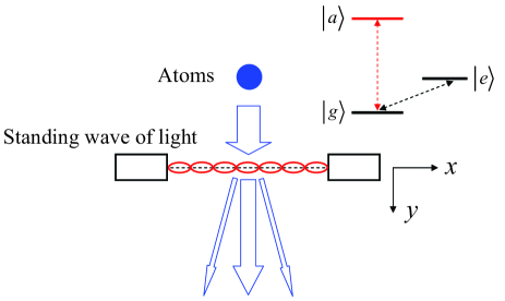
Figure 1: State-selective scattering of the three-level V-type atoms. An incident Gaussian beam of atoms is scattered transversely by the standing wave of light, resulting in a large momentum uncertainty of spatially coherent atoms. The atomic KD scattering occurs within the near-resonant regime of optical transition $|g\rangle\rightleftharpoons|a\rangle$. When atoms are initially in the internal state $|e\rangle$, the scattering is negligible. This provides an effective approach to measure the qubits $|g\rangle$ and $|e\rangle$ by observing the external c.m. momenta of atoms.

Considering the atomic Gaussian beam incident, the external $x$-directional motion is initially in the state of

$$|0\rangle=c\int_{-\infty}^{\infty}e^{\frac{-x^{2}}{4\Delta^{2}}}|x\rangle dx=c^{\prime}\int_{-\infty}^{\infty}e^{\frac{-p_{x}^{2}}{4\sigma^{2}}}|p_{x}\rangle dp_{x}\,.$$ (26)

Here, $c=(2\pi\Delta^{2})^{-1/4}$ and $c^{\prime}=(2\pi\sigma^{2})^{-1/4}$ are the normalized coefficients, and $|x\rangle$ and $|p_{x}\rangle$ are respectively the atomic position and momentum eigenstates. The quantities $\Delta$ and $\sigma=\hbar/(2\Delta)$ are the atomic position and momentum uncertainty, respectively. Obviously, the large position uncertainty corresponds to a small momentum uncertainty. If the internal state of the atoms is initially in the ground state $|g\rangle$, the scattered state reads KD1

$$|{\rm KD}\rangle=e^{-i\Omega\tau\sin^{2}(kx)}|0\rangle=e^{i\eta\cos(2kx)}|0\rangle\,.$$ (27)

In short, we have denoted $\Omega\tau/2=\eta$ and neglected the phase $\exp[-i\hat{p}_{x}^{2}\tau/(2m\hbar)]\exp(-i\eta)$. Expanding $\exp[i\eta\cos(2kx)]$ by the Bessel functions $J_{n}(\eta)$ of the first kind, the atomic external motion reads

$$|{\rm KD}\rangle=\sum_{n=-\infty}^{\infty}\phi(n)e^{i2nkx}|0\rangle\,,$$ (28)

with $\phi(n)=i^{n}J_{n}(\eta)$. Above, the term $\exp(i2nkx)$ acts as a momentum-displacement operator in the $x$ direction, i.e.,

$$e^{i2nkx}|0\rangle=|n\rangle=c^{\prime}\int_{-\infty}^{\infty}e^{-\frac{(p_{x}-2n\hbar k)^{2}}{4\sigma^{2}}}|p_{x}\rangle dp_{x}\,.$$ (29)

If the initial momentum uncertainty is small, i.e., $\sigma\ll\hbar k$, the states $\{|n\rangle\}$ can be regarded as the orthonormal basis, i.e., $\langle n^{\prime}|n\rangle=\delta_{n^{\prime},n}$ (with $\delta_{n^{\prime},n}$ being the Kronecker delta function). Numerically, considering the atomic position uncertainty $\Delta=1~{}\mu$m and the wavelength $\lambda=0.4~{}\mu$m of a visible light, we have $\hbar k/\sigma=4\pi\Delta/\lambda\approx 31$ and $\langle 0|1\rangle=\exp[-(\hbar k)^{2}/(2\sigma^{2})]=\exp(-480.5)$. It can be further found that $\langle n^{\prime}|\hat{p}_{x}^{2}|n\rangle\approx(2n\hbar k)^{2}\delta_{n^{\prime},n}$, such that the momentum uncertainty of the scattered atoms is calculated as $\langle\phi_{x}|\hat{p}_{x}^{2}|\phi_{x}\rangle=(2\hbar k)^{2}\vartheta$ KD1 ; KD2 ; KD3 . Where, the quantity $\vartheta=\sum_{-\infty}^{\infty}n^{2}J_{n}^{2}$ can be directly computed by the numerical method, for example, $\vartheta=50$ with $\eta=10$.

The detection of momentum states $\{|n\rangle\}$ is similar to that of the classical particles, by directly observing their distinguishable paths. Considering the free diffraction, we replace Eq. (28) by

$$|\phi_{x}\rangle=e^{\frac{-it_{0}\hat{p}^{2}_{x}}{2m\hbar}}|{\rm KD}\rangle=\sum_{n=-\infty}^{\infty}\phi(n)|\tilde{n}\rangle\,.$$ (30)

Here, $t_{0}=\tau+\tau^{\prime}$, with $\tau^{\prime}$ being the time after the light driving. For the time-dependent momentum state $|\tilde{n}\rangle=\exp[-it_{0}\hat{p}_{x}^{2}/(2m\hbar)]|n\rangle$, its wave packet $|\langle x|\tilde{n}\rangle|^{2}$ spreads with a quantity $\Delta_{d}=\hbar t_{0}/(2m\Delta)$ which is smaller than the shift $D_{n}=4n\pi\hbar t_{0}/(m\lambda)$ of the wave-packet center (because $\Delta>\lambda$). Hence, the states $\{|\tilde{n}\rangle\}$ can be distinguishable in position space when the time $\tau^{\prime}$ is sufficiently long, i.e., $D_{n}\gg\sqrt{\Delta^{2}+\Delta^{2}_{d}}$. The atoms beam in momentum state $|\tilde{n}\rangle$ can be directly observed by placing a detector at the position $D_{n}$ (with a collecting region $\sim\sqrt{\Delta^{2}+\Delta^{2}_{d}}$).

IV.2 The postselection

The desired postselection of internal state $|A_{s}\rangle$ can be realized by the following two steps. First, we perform a single-qubit rotation $\hat{R}=\exp[-i\theta(|e\rangle\langle g|+|g\rangle\langle e|)]$ to the atomic internal state by the Raman beams. The parameter $\theta$ is a controllable quantity which is proportional to the power and duration of the drivings. For simplicity, we assume that the single-qubit operations do not affect the $x$-directional c.m. motions. This can be realized by properly selecting the direction of laser irradiating, e.g., the $y$ direction. Second, we use another laser to realize the KD scattering of atoms, i.e., the Hamiltonian $\hat{H}_{ac}$. Since the effective interaction occurs between the transition $|a\rangle\leftrightharpoons|g\rangle$, the scattering is state-selective. If the atom is in state $|e\rangle$, there is no KD scattering. However, the atoms in state $|g\rangle$ will be scattered and consequently deviate from their original trajectory to be detected. Worthy of note is that the present postselection is similar to that in the original work AAV by Aharonov et al. There, a Stern-Gerlach device is arranged to implemented the postselection of electronic spin. It couples the spin to the orbital motions of the electron. Consequently, they select an orbital motion to realize the postselection of the electronic spin state. Here, we use a state-dependent KD scattering to implement the desired postselection of the atomic internal state. Supposing the total duration of the above two operations is sufficiently short (i.e., the interaction of $g_{0}$ in this stage is negligible), the desired postselection operation $\langle g|\hat{R}$ can be realized. For such a postselection, the weak value reads

$$A_{w}=\frac{\langle g|\hat{R}|e\rangle\langle e|A^{\prime}_{i}\rangle}{\langle g|\hat{R}|A^{\prime}_{i}\rangle}=\frac{\beta}{\beta+ie^{i\omega t}\alpha\cot(\theta)}$$ (31)

with the initial state $|A_{i}\rangle=\alpha|g\rangle+\beta|e\rangle$. Obviously, the real or imaginary part of the above weak value can be nonzero. That is, the single-qubit operations in state preparation and postselection will change the final results of detection. In particular, if $\alpha=\beta=1/\sqrt{2}$, $\theta=3\pi/4$, and $\omega t\rightarrow(2n-1/2)\pi$ Miao , we have $A_{w}^{i}\rightarrow\infty$. Of course, the relevant qualities such as the durations of laser pulses should be exactly controlled in experiments, like the well-known Ramsey interferometers atomoptics .

IV.3 The weak-value amplification

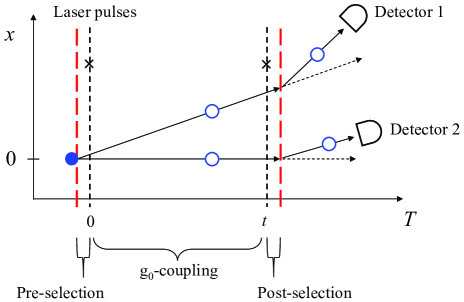
Figure 2: A flow chart of weak measurement. The preselection (state preparation) includes two steps, the KD scattering for atomic external state preparation and the single-qubit operation for internal superposition state generation. After a duration of $g_{0}$ coupling, the postselection is implemented by the other single-qubit operation and KD scattering. The momentum distribution of the scattered atoms depends on the parameter $g_{0}$ and the imaginary part of the weak value. By comparing the intensities of the selected two atomic beams the parameter $g_{0}$ could be estimated.

The considered weak measurement process is diagrammatically shown in Fig. 2. The atoms undergo the following several stages: (a) standing light wave induced KD scattering in the $x$ direction, (b) single-qubit operation performed by the $y$-directional laser beams, (c) the $g_{0}$ couplings, (d) postselection implemented by the other single-qubit operation and KD scattering, and (e) the final detection. In fact, steps (a) and (b) are those for the initial state preparations of both the atomic internal and external degrees of freedom.

Regarding (30) as the external initial state of atoms, the single-qubit operation was performed to generate the desired internal state, i.e., $|g\rangle\rightarrow|A_{i}\rangle$. After a duration of $g_{0}$ coupling, the postselection was performed on the atomic internal state, resulting in state (22). Directly, putting the prepared state (30) into Eq. (22), we have

$$|f\rangle= \langle A_{s}|A^{\prime}_{i}\rangle\hat{V}_{t}\left[1+\frac{iA_{w}g_{0}t}{2m\hbar}(\hat{p}^{2}-2m\hat{G})\right]\sum_{n=-\infty}^{\infty}\phi(n)|\tilde{n}\rangle$$ (32)

$$\otimes|\phi_{y}\rangle|\phi_{z}\rangle\,.$$

Under the approximation $\langle\tilde{n}^{\prime}|\hat{p}_{x}^{2}|\tilde{n}\rangle=\langle n^{\prime}|\hat{p}_{x}^{2}|n\rangle\approx(2n\hbar k)^{2}\delta_{n^{\prime},n}$, the probability of finding the momentum state $|\tilde{n}\rangle$ is calculated as

$$P_{n} =P_{s}\frac{|\langle\tilde{n}|f\rangle|^{2}}{\langle f|f\rangle}=|\langle\tilde{n}|f\rangle|^{2}$$ (33)

$$=|\langle A_{s}|A^{\prime}_{i}\rangle|^{2}J_{n}^{2}\left\{1-\frac{g_{0}tA_{w}^{i}}{m\hbar}\left[(2n\hbar k)^{2}+\langle yz\rangle\right]\right\}$$

Here, the postselection probability $P_{s}$ is induced, i.e., our statistics is based on the entire atomic ensemble. The term $\langle yz\rangle=\langle i|(\hat{p}_{y}^{2}+\hat{p}_{z}^{2}-2m\hat{G})|i\rangle$ refers to $y$ and $z$ directional motions. Its contribution for Eq. (33) is small because momentum uncertainties in the $y$ and $z$ directions were not enhanced. Due to the limited interaction time $t$, the contribution from gravity could be also negligible. Therefore, Eq. (33) can be reduced as

$$P_{n}=|\langle A_{s}|A^{\prime}_{i}\rangle|^{2}J_{n}^{2}(1-g_{0}\omega_{k}tn^{2}A^{i}_{w})\,,$$ (34)

by neglecting the term $\langle yz\rangle$, where $\omega_{k}=4\hbar k^{2}/m$. The above equation indicates that the imaginary part of the weak value will change the momentum distribution of the post-selected atoms. This provides us an alternative approach to measure the parameter $g_{0}$. As we mentioned earlier, the postselection probability $P_{s}$ is also an effective measurement for $g_{0}$, if the number $N$ of the input atoms is precise. Similarly, by neglecting the contribution from $y$- and $z$-directional motions, we have

$$P_{s}=|\langle A_{s}|A^{\prime}_{i}\rangle|^{2}(1-g_{0}\omega_{k}t\vartheta A^{i}_{w})\,,$$ (35)

which satisfies the normalized condition $\sum_{n=-\infty}^{\infty}P_{n}=P_{s}$.

The usefulness of the weak value is significant: it can amplify the $g_{0}$ signal with the respective of backgrounds [i.e., the first terms in Eqs. (34) and (35)]. Generally, the output of an atom-detector can be described by the equation $I_{n}=(N+\xi_{s})P_{n}+(N+\xi_{s})\xi_{d}P_{n}+\varepsilon$. Here, $\xi_{s}$ is an uncertainty of input atoms (namely, the source-noise), $\xi_{d}$ denotes the uncertainty of detection efficiency (such as the detector saturation). In other words, $\xi_{d}$ is the noise which is proportional to the amount of received atoms. $\varepsilon$ denotes the dark-counting which is $N+\xi_{s}$ independent. A single atom can be easily observed by its resonance fluorescence, so that the dark-counting $\varepsilon$ is negligible. The main noises in the atomic system are $\xi_{s}$ and $\xi_{d}$. Using the weak-value amplification, the background-induced noises, e.g., $N|\langle A_{s}|A^{\prime}_{i}\rangle|^{2}\xi_{d}$, will be significantly suppressed.

Comparing to postselection probability $P_{s}$, the momentum distribution $P_{n}$ of the post-selected atoms is more useful for suppressing the source-noise. One can use two detectors to measure such a distribution, for example,

$$\frac{I_{n}}{I_{0}} =\frac{(1+\xi_{1d})P_{n}}{(1+\xi_{2d})P_{0}}$$ (36)

$$\approx(1+\xi_{1d}-\xi_{2d})\left(1-g_{0}\omega_{k}tn^{2}A^{i}_{w}\right)\frac{J_{n}^{2}}{J_{0}^{2}}\,.$$

Where, the source-noise (and the term $|\langle A_{s}|A^{\prime}_{i}\rangle|^{2}$) has been completely eliminated, and $(1+\xi_{1d})/(1+\xi_{2d})\approx 1+\xi_{1d}-\xi_{2d}$ is due to the noises of two detectors (denoted by, respectively, $\xi_{1d}$ and $\xi_{1d}$). The imaginary part of the weak value can be an evidence for the coupling of $|e\rangle\langle e|p^{2}$. If there is no such coupling (i.e., replacing $|e\rangle\langle e|$ by the unit operator $\hat{1}$), the weak value $A_{w}^{i}=0$ and consequently the Eq. (36) is $g_{0}$ independent. In principle, when $g_{0}\omega_{k}tn^{2}A^{i}_{w}>\xi_{1d},\,\xi_{2d}$, the signal of $g_{0}$ should be detectable.

Both Eq. (34) and (35) indicate $g_{0}\omega_{k}t$ is a very crucial quantity for measuring the parameter $g_{0}$. Such a quality depends on $k^{2}$, so that using the high-frequency light scattering can significantly enhance the desired signal of $g_{0}$. Of course, $g_{0}t=\hbar\omega t/(mc^{2})$ is the most basic quality. Where, the interaction duration $t$ is limited within the coherent times of the atomic qubit. Hence, the optical atomic clocks are perhaps the good candidates for the relatively large $g_{0}t$ gain, because they have the qualities of both large transition frequency $\omega$ and long lifetime $t$ Ca1 ; Ca2 ; Ca3 . Considering the usually used transition ${}^{1}S_{0}-^{3}P_{1}$ of a calcium clock, the resonant frequency and the lifetime of the excited state ${}^{3}P_{1}$ are respectively $\omega\approx 4.6\times 10^{14}$ Hz and $t\approx 0.4$ ms Ca1 , such that $g_{0}t\approx 3.2\times 10^{-15}$ s. The relatively strong KD scattering occurs at the transition ${}^{1}S_{0}-^{1}P_{1}$ of calcium, and where the wavelength of the driving light is on the order of $\lambda=2\pi/k\approx 0.4~{}\mu$m. Using these parameters, we have $\omega_{k}\approx 1.6$ MHz and $g_{0}\omega_{k}t\approx 5\times 10^{-9}$. Considering a KD scattering with $\eta=10$, the probability for finding momentum $|n=10\rangle$ is $J^{2}_{10}(\eta)\approx 0.04$. As a consequence, $g_{0}\omega_{k}tn^{2}A_{w}^{i}\approx 5\times 10^{-3}$ is obtained by selecting a large weak value $A_{w}^{i}=1\times 10^{4}$. Such a signal may be detectable if the noises $\xi_{1d}$ and $\xi_{2d}$ are smaller than $5\times 10^{-3}$. Note that, the present weak measurement is also suitable for some other scattering mechanisms, for example, preparing the atomic initial state with more large momentum uncertainty by the multi-step scattering of lights. In principle, this will generate more significant effects of $g_{0}$ than the present one.

V Conclusion

In this theoretical work, we proposed a weak value scheme to measure the effect of mass-energy equivalence in the system of coherent atoms. First, we reviewed briefly the principle of quantum weak measurement and its usefulness in the weak signal detections. Second, we presented an approach to derive the dynamic evolution of an atom whose internal and external degrees of freedom are coupled due to the mass-energy equivalence. After a duration of such a coupling, the weak value is obtained by post-selecting an atomic internal state. It is shown that the imaginary part of the weak value can change the momentum distribution of the selected atoms. This allowed us to measure the coupling of mass-energy equivalence in the momentum space of atoms. Third, we used the KD scattering to prepare and post-select the atoms (with the help of two single-qubit rotations). Preparing atomic momentum states by the light-induced scattering is optimal for measuring the coupling of $|e\rangle\langle e|\hat{p}^{2}$, because the scattering can generate a relatively large momentum uncertainty of coherent atoms. Certainly, observing the effect of this coupling is still difficult by using even advanced optical atomic clocks. Under this situation, the weak value would be useful. It can significantly amplify the signals above the background noises, making the detection of weak signals feasible. Finally, we hope the present studies will encourage further studies on the detection of weak signals.

Acknowledgements: This work was partly supported by the National Natural Science Foundation of China, Grants No. 11204249 and No. 11547311.

References

- (1) Y. Aharonov, D. Z. Albert, and L. Vaidman, “How the result of a measurement of a component of the spin of a spin- particle can turn out to be 100”, Phys. Rev. Lett. 60, 1351 (1988).
- (2) R. Jozsa, “Complex weak values in quantum measurement”, Phys. Rev. A 76, 044103 (2007).
- (3) J. Dressel and A. N. Jordan, “Significance of the imaginary part of the weak value”, Phys. Rev. A 85, 012107 (2012).
- (4) M. F. Pusey, “Anomalous weak values are proofs of contextuality”, Phys. Rev. Lett. 113, 200401 (2014).
- (5) J. S. Lundeen, B. Sutherland, A. Patel, C. Stewart, and C. Bamber, “Direct measurement of the quantum wavefunction”, Nature (London) 474, 188 (2011).
- (6) S. Kocsis, B. Braverman, S. Ravets, M. J. Stevens, R. P. Mirin, L. K. Shalm, and A. M. Steinberg, “Observing the average trajectories of single photons in a two-slit interferometer”, Science 332, 1170 (2011).
- (7) J. S. Lundeen and A. M. Steinberg, “Experimental joint weak measurement on a photon pair as a probe of Hardy’s paradox”, Phys. Rev. Lett. 102, 020404 (2009).
- (8) J. Dressel, C. J. Broadbent, J. C. Howell, and A. N. Jordan, “Experimental violation of two-party Leggett-Garg inequalities with semiweak measurements”, Phys. Rev. Lett. 106, 040402 (2011).
- (9) O. Hosten and P. Kwiat P, “Observation of the spin Hall effect of light via weak measurements”, Science 319, 787 (2008).
- (10) Y. Aharonov, S. Popescu, D. Rohrlich, and P. Skrzypczyk, “Quantum Cheshire Cats”, New J. Phys. 15, 113015 (2013).
- (11) T. Denkmayr, H. Geppert, S. Sponar, H. Lemmel, A. Matzkin, J. Tollaksen, and Y. Hasegawa, “Observation of a quantum Cheshire cat in a matter-wave interferometer experiment”, Nat. Commun. 5, 4492 (2014).
- (12) R. Corrêa, M. F. Santos, C. H. Monken, and P. L. Saldanha, “‘Quantum Cheshire Cat’ as simple quantum interference”, New J. Phys. 17, 053042 (2015).
- (13) N. Brunner, V. Scarani, M. Wegmüller, M. Legré, and N. Gisin, “Direct measurement of superluminal group velocity and signal velocity in an optical fiber”, Phys. Rev. Lett. 93, 203902 (2004).
- (14) D. Rohrlich and Y. Aharonov, “Cherenkov radiation of superluminal particles”, Phys. Rev. A 66, 042102 (2002).
- (15) M. V. Berry, “Superluminal speeds for relativistic random waves”, J. Phys. A: Math. Theor. 45, 185308 (2012).
- (16) A. M. Steinberg, “How much time does a tunneling particle spend in the barrier region?”, Phys. Rev. Lett. 74, 2405 (1995).
- (17) D. Marian, N. Zanghì, and X. Oriols, “Weak values from displacement currents in multiterminal electron devices”, Phys. Rev. Lett. 116, 110404 (2016).
- (18) P. B. Dixon, D. J. Starling, A. N. Jordan, and J. C. Howell, “Ultrasensitive beam deflection measurement via interferometric weak value amplification”, Phys. Rev. Lett. 102, 173601 (2009).
- (19) O. S. Magaña-Loaiza, M. Mirhosseini, B. Rodenburg, and R. W. Boyd, “Amplification of angular rotations using weak measurements”, Phys. Rev. Lett. 112, 200401 (2014).
- (20) S. Pang, J. Dressel, and T. A. Brun, “Entanglement-assisted weak value amplification”, Phys. Rev. Lett. 113, 030401 (2014).
- (21) A. Feizpour, X. Xing, and A. M. Steinberg, “Amplifying single-photon nonlinearity using weak measurements”, Phys. Rev. Lett. 107, 133603 (2011).
- (22) Y. Susa, Y. Shikano, and A. Hosoya, “Optimal probe wave function of weak-value amplification”, Phys. Rev. A 85, 052110 (2012).
- (23) G. B. Alves, B. M. Escher, R. L. de Matos Filho, N. Zagury, and L. Davidovich “Weak-value amplification as an optimal metrological protocol”, Phys. Rev. A 91, 062107 (2015).
- (24) G. I. Viza, J. Martínez-Rincón, G. B. Alves, A. N. Jordan, and J. C. Howell, “Experimentally quantifying the advantages of weak-value-based metrology”, Phys. Rev. A 92, 032127 (2015).
- (25) O. Zilberberg, A. Romito, and Y. Gefen, “Charge sensing amplification via weak values measurement”, Phys. Rev. Lett. 106, 080405 (2011).
- (26) J. P. Torres and L. J. Salazar-Serrano, “Weak value amplification: a view from quantum estimation theory that highlights what it is and what isn’t”, Sci. Rep. 6, 19702 (2016).
- (27) J. Dressel, M. Malik, F. M. Miatto, A. N. Jordan, and R. W. Boyd, “Understanding quantum weak values: Basics and applications”, Rev. Mod. Phys. 86, 307 (2014).
- (28) S. Sponar, T. Denkmayr, H. Geppert, H. Lemmel, A. Matzkin, J. Tollaksen, and Y. Hasegawa, “Weak values obtained in matter-wave interferometry”, Phys. Rev. A 92, 062121 (2015).
- (29) S. Rainville, J. K. Thompson, E. G. Myers, J. M. Brown, M. S. Dewey, E. G. Kessler, R. D. Deslattes, H. G. Börner, M. Jentschel, P. Mutti, and D. E. Pritchard, “World Year of Physics: A direct test of E=mc2”, Nature (London) 438, 1096 (2005).
- (30) M. Zych, F. Costa, I. Pikovski, and Č. Brukner, “Quantum interferometric visibility as a witness of general relativistic proper time”, Nat. Commun. 2, 505 (2011).
- (31) M. Zych and Č. Brukner, “Quantum formulation of the Einstein Equivalence Principle”, arXiv:1502.00971.
- (32) I. Pikovski, M. Zych, F. Costa, and Č. Brukner, “Universal decoherence due to gravitational time dilation”, Nat. Phys. 11, 668 (2015).
- (33) D. E. Krause and I. Lee, “Taking Einstein seriously: Relativistic coupling of internal and center of mass dynamics”, arXiv:1608.03253v1.
- (34) P. J. Orlando, R. B. Mann, K. Modi, and F. A. Pollock, “A test of the equivalence principle(s) for quantum superpositions”, Class. Quantum Grav. 33, 19LT01 (2016).
- (35) J. C. Hafele and R. E. Keating, “Around-the-world atomic clocks: observed relativistic time gains”, Science, 177, 168 (1972).
- (36) H. Müller, A. Peters, and S. Chu, “A precision measurement of the gravitational redshift by the interference of matter waves”, Nature (London), 463, 926 (2010).
- (37) H. Müeller, “Quantum mechanics, matter waves, and moving clocks”, in Proceedings of the International School of Physics “Enrico Fermi”, Course 188 “Atom Interferometry”, edited by G. M. Tino and M. A. Kasevich (IOS press, Amsterdam, 2014), p. 339.
- (38) J. Audretsch, U. Bleyer, and C. Lämmerzahl, “Testing Lorentz invariance with atomic-beam interferometry”, Phys. Rev. A, 47, 4632 (1993).
- (39) A. D. Cronin, J. Schmiedmayer, and D. E. Pritchard, “Optics and interferometry with atoms and molecules”, Rev. Mod. Phys. 81, 1051 (2009).
- (40) C. Ferrie and J. Combes, “Weak value amplification is suboptimal for estimation and detection”, Phys. Rev. Lett. 112, 040406 (2014).
- (41) G. C. Knee and E. M. Gauger, “When amplification with weak values fails to suppress technical noise”, Phys. Rev. X 4, 011032 (2014).
- (42) G. C. Knee, J. Combes, C. Ferrie, and E. M. Gauger, “Weak-value amplification: state of play”, Quantum Meas. Quantum Metrol. 3, 32 (2016).
- (43) A. N. Jordan, J. Martínez-Rincón, and J. C. Howell, “Technical advantages for weak-value amplification: when less is more”, Phys. Rev. X 4, 011031 (2014).
- (44) X. Zhu, Y. Zhang, S. Pang, C. Qiao, Q. Liu, and S. Wu, “Quantum measurements with preselection and postselection ”, Phys. Rev. A 84, 052111 (2011).
- (45) M. Zhang and S. Y. Zhu, “Application of the weak-measurement technique to study atom-vacuum interactions”, Phys. Rev. A 92, 043825 (2015).
- (46) L. Viola and R. Onofrio, “Testing the equivalence principle through freely falling quantum objects”, Phys. Rev. D 55, 455 (1997).
- (47) S. Fray, C. A. Diez, T. W. Hänsch, and M. Weitz, “Atomic interferometer with amplitude gratings of light and its applications to atom based tests of the equivalence principle”, Phys. Rev. Lett. 93, 240404 (2004).
- (48) S. Gupta, A. E. Leanhardt, A. D. Cronin, and D. E. Pritchard, “Coherent manipulation of atoms with standing light waves”, C. R. Acad. Sci. Series IV 2, 479 (2001).
- (49) P. L. Gould, G. A. Ruff, and D. E. Pritchard, “Diffraction of atoms by light: the near-resonant Kapitza-Dirac effect”, Phys. Rev. Lett. 56, 827 (1986).
- (50) Yu. B. Ovchinnikov, J. H. Müller, M. R. Doery, E. J. D. Vredenbregt, K. Helmerson, S. L. Rolston, and W. D. Phillips, “Diffraction of a released Bose-Einstein condensate by a pulsed standing light wave”, Phys. Rev. Lett. 83, 284 (1999).
- (51) F. Riehle, Th. Kisters, A. Witte, J. Helmcke, and Ch. J. Bordé, “Optical Ramsey spectroscopy in a rotating frame: Sagnac effect in a matter-wave interferometer”, Phys. Rev. Lett. 67, 177 (1991).
- (52) A. D. Ludlow, M. M. Boyd, and J. Ye, “Optical atomic clocks”, Rev. Mod. Phys. 87, 637 (2015).
- (53) T. Binnewies, G. Wilpers, U. Sterr, F. Riehle, J. Helmcke, T. E. Mehlstäubler, E. M. Rasel, and W. Ertmer, “Doppler cooling and trapping on forbidden transitions”, Phys. Rev. Lett. 87, 123002 (2001).