LP-based Tractable Subcones of the Semidefinite Plus Nonnegative Cone

Abstract

The authors in a previous paper devised certain subcones of the semidefinite plus nonnegative cone and showed that satisfaction of the requirements for membership of those subcones can be detected by solving linear optimization problems (LPs) with $O(n)$ variables and $O(n^{2})$ constraints. They also devised LP-based algorithms for testing copositivity using the subcones. In this paper, they investigate the properties of the subcones in more detail and explore larger subcones of the positive semidefinite plus nonnegative cone whose satisfaction of the requirements for membership can be detected by solving LPs. They introduce a semidefinite basis (SD basis) that is a basis of the space of $n\times n$ symmetric matrices consisting of $n(n+1)/2$ symmetric semidefinite matrices. Using the SD basis, they devise two new subcones for which detection can be done by solving LPs with $O(n^{2})$ variables and $O(n^{2})$ constraints. The new subcones are larger than the ones in the previous paper and inherit their nice properties. The authors also examine the efficiency of those subcones in numerical experiments. The results show that the subcones are promising for testing copositivity as a useful application.

Key words. Semidefinite plus nonnegative cone, Doubly nonnegative cone, Copositive cone, Matrix decomposition, Linear programming, Semidefinite basis, Maximum clique problem, Quadratic optimization problem

1 Introduction

Let $\mathcal{S}_{n}$ be the set of $n\times n$ symmetric matrices, and define their inner product as

$$\langle A,B\rangle={\rm Tr}\,(B^{T}A)=\sum_{i.j=1}^{n}a_{ij}b_{ij}.$$ (1)

Bomze et al. [7] coined the term “copositive programming” in relation to the following problem in 2000, on which many studies have since been conducted:

$$\begin{array}[]{ll}\mbox{Minimize}&\langle C,X\rangle\\ \mbox{subject to}&\langle A_{i},X\rangle=b_{i},\ (i=1,2,\ldots,m)\\ &X\in{\cal COP}_{n}.\end{array}$$

where $\mathcal{COP}_{n}$ is the set of $n\times n$ copositive matrices, i.e., matrices whose quadratic form takes nonnegative values on the $n$-dimensional nonnegative orthant $\mathbb{R}^{n}_{+}$:

$$\mathcal{COP}_{n}:=\{X\in\mathcal{S}_{n}\mid d^{T}Xd\geq 0\ \mbox{for all}\ d\in\mathbb{R}^{n}_{+}\}.$$

We call the set $\mathcal{COP}_{n}$ the copositive cone. A number of studies have focused on the close relationship between copositive programming and quadratic or combinatorial optimization (see, e.g., [7][8][15][33][34][13][14][20]). Interested readers may refer to [21] and [9] for background on and the history of copositive programming.

The following cones are attracting attention in the context of the relationship between combinatorial optimization and copositive optimization (see, e.g., [21][9]). Here, ${\rm conv}\,(S)$ denotes the convex hull of the set $S$.

-

The nonnegative cone ${\cal N}_{n}:=\left\{X\in\mathcal{S}_{n}\mid x_{ij}\geq 0\mbox{ for all}\ i,j\in\{1,2,\ldots,n\}\right\}$.

-

The semidefinite cone ${\cal S}_{n}^{+}:=\{X\in\mathcal{S}_{n}\mid d^{T}Xd\geq 0\ \mbox{for all}\ d\in\mathbb{R}^{n}\}={\rm conv}\,\left(\left\{xx^{T}\mid x\in\mathbb{R}^{n}\right\}\right)$.

-

The copositive cone ${\cal COP}_{n}:=\left\{X\in\mathcal{S}_{n}\mid d^{T}Xd\geq 0\ \mbox{ for all}\ d\in\mathbb{R}^{n}_{+}\right\}$.

-

The semidefinite plus nonnegative cone ${\cal S}_{n}^{+}+{\cal N}_{n}$, which is the Minkowski sum of ${\cal S}_{n}^{+}$ and ${\cal N}_{n}$.

-

The union ${\cal S}_{n}^{+}\cup{\cal N}_{n}$ of ${\cal S}_{n}^{+}$ and ${\cal N}_{n}$.

-

The doubly nonnegative cone ${\cal S}_{n}^{+}\cap{\cal N}_{n}$, i.e., the set of positive semidefinite and componentwise nonnegative matrices.

-

The completely positive cone ${\cal CP}_{n}:={\rm conv}\,\left(\left\{xx^{T}\mid x\in\mathbb{R}^{n}_{+}\right\}\right)$.

Except the set ${\cal S}_{n}^{+}\cup{\cal N}_{n}$, all of the above cones are proper (see Section 1.6 of [5], where a proper cone is called a full cone), and we can easily see from the definitions that the following inclusions hold:

$${\cal COP}_{n}\supseteq{\cal S}_{n}^{+}+{\cal N}_{n}\supseteq{\cal S}_{n}^{+}\cup{\cal N}_{n}\supseteq{\cal S}_{n}^{+}\supseteq{\cal S}_{n}^{+}\cap{\cal N}_{n}\supseteq{\cal CP}_{n}.$$ (2)

While copositive programming has the potential of being a useful optimization technique, it still faces challenges. One of these challenges is to develop efficient algorithms for determining whether a given matrix is copositive. It has been shown that the above problem is co-NP-complete [31][19][20] and many algorithms have been proposed to solve it (see, e.g., [6][12][30][29][39][36][10][16][22][37][11]) Here, we are interested in numerical algorithms which (a) apply to general symmetric matrices without any structural assumptions or dimensional restrictions and (b) are not merely recursive, i.e., do not rely on information taken from all principal submatrices, but rather focus on generating subproblems in a somehow data-driven way, as described in [10]. There are few such algorithms, but they often use tractable subcones $\mathcal{M}_{n}$ of the semidefinite plus nonnegative cone ${\cal S}_{n}^{+}+{\cal N}_{n}$ for detecting copositivity (see, e.g., [12][36][10][37]). As described in Section 5, these algorithms require one to check whether $A\in\mathcal{M}_{n}$ or $A\not\in\mathcal{M}_{n}$ repeatedly over simplicial partitions. The desirable properties of the subcones $\mathcal{M}_{n}\subseteq{\cal S}_{n}^{+}+{\cal N}_{n}$ used by these algorithms can be summarized as follows:

P1

For any given $n\times n$ symmetric matrix $A\in\mathcal{S}_{n}$, we can check whether $A\in\mathcal{M}_{n}$ within a reasonable computation time, and

P2

$\mathcal{M}_{n}$ is a subset of the semidefinite plus nonnegative cone ${\cal S}_{n}^{+}+{\cal N}_{n}$ that at least includes the $n\times n$ nonnegative cone $\mathcal{N}_{n}$ and contains as many elements ${\cal S}_{n}^{+}+{\cal N}_{n}$ as possible.

The authors, in [37], devised certain subcones of the semidefinite plus nonnegative cone ${\cal S}_{n}^{+}+{\cal N}_{n}$ and showed that satisfaction of the requirements for membership of those cones can be detected by solving linear optimization problems (LPs) with $O(n)$ variables and $O(n^{2})$ constraints. They also created an LP-based algorithm that uses these subcones for testing copositivity as an application of those cones.

The aim of this paper is twofold. First, we investigate the properties of the subcones in more detail, especially in terms of their convex hulls. Second, we search for subcones of the semidefinite plus nonnegative cone ${\cal S}_{n}^{+}+{\cal N}_{n}$ that have properties P1 and P2. To address the second aim, we introduce a semidefinite basis (SD basis) that is a basis of the space $\mathcal{S}_{n}$ consisting of $n(n+1)/2$ symmetric semidefinite matrices. Using the SD basis, we devise two new types of subcones for which detection can be done by solving LPs with $O(n^{2})$ variables and $O(n^{2})$ constraints. As we will show in Corollary 3.4, these subcones are larger than the ones proposed in [37] and inherit their nice properties. We also examine the efficiency of those subcones in numerical experiments.

This paper is organized as follows: In Section 2, we show several tractable subcones of ${\cal S}_{n}^{+}+{\cal N}_{n}$ that are receiving much attention in the field of copositive programming and investigate their properties, the results of which are summarized in Figures 1 and 2. In Section 3, we propose new subcones of ${\cal S}_{n}^{+}+{\cal N}_{n}$ having properties P1 and P2. We define SD bases using Definitions 3.2 and 3.3 and construct new LPs for detecting whether a given matrix belongs to the subcones. In Section 4, we perform numerical experiments in which the new subcones are used for identifying the given matrices $A\in\mathcal{S}_{n}^{+}+\mathcal{N}_{n}$. As a useful application of the new subcones, Section 5 describes experiments for testing copositivity of matrices arising from the maximum clique problem and standard quadratic optimization problems. The results of these experiments show that the new subcones are promising not only for identification of $A\in\mathcal{S}_{n}^{+}+\mathcal{N}_{n}$ but also for testing copositivity. We give concluding remarks in Section 6.

2 Some tractable subcones of ${\cal S}_{n}^{+}+{\cal N}_{n}$ and related work

In this section, we show several tractable subcones of the semidefinite plus nonnegative cone ${\cal S}_{n}^{+}+{\cal N}_{n}$. Since the set ${\cal S}_{n}^{+}+{\cal N}_{n}$ is the dual cone of the doubly nonnegative cone ${\cal S}_{n}^{+}\cap{\cal N}_{n}$, we see that

$${\cal S}_{n}^{+}+{\cal N}_{n} = \{A\in{\cal S}_{n}\mid\langle A,X\rangle\geq 0\ \mbox{for any}\ X\in{\cal S}_{n}^{+}\cap{\cal N}_{n}\}$$

$$= \{A\in{\cal S}_{n}\mid\langle A,X\rangle\geq 0\ \mbox{for any}\ X\in{\cal S}_{n}^{+}\cap{\cal N}_{n}\ \mbox{such that}\ {\rm Tr}\,(X)=1\}$$

and that the weak membership problem for ${\cal S}_{n}^{+}+{\cal N}_{n}$ can be solved (to an accuracy of $\epsilon$) by solving the following doubly nonnegative program (which can be expressed as a semidefinite program of size $O(n^{2})$).

$$\begin{array}[]{ll}\mbox{Minimize}&\langle A,X\rangle\\ \mbox{subject to}&\langle I_{n},X\rangle=1,\ X\in{\cal S}_{n}^{+}\cap{\cal N}_{n}\end{array}$$ (3)

where $I_{n}$ denotes the $n\times n$ identity matrix. Thus, the set ${\cal S}_{n}^{+}+{\cal N}_{n}$ is a rather large and tractable convex subcone of $\mathcal{COP}_{n}$. However, solving the problem takes a lot of time [36], [38] and does not make for a practical implementation in general. To overcome this drawback, more easily tractable subcones of ${\cal S}_{n}^{+}+{\cal N}_{n}$ have been proposed.

We define the matrix functions $N,S:{\cal S}_{n}\rightarrow{\cal S}_{n}$ such that, for $A\in\mathcal{S}_{n}$, we have

$$N(A)_{ij}:=\left\{\begin{array}[]{ll}A_{ij}&\ \ (A_{ij}>0\ \mbox{and}\ i\neq j)\\ 0&\ \ (\mbox{otherwise})\end{array}\right.\ \ \mbox{and}\ \ S(A):=A-N(A).$$ (4)

In [36], the authors defined the following set:

$$\mathcal{H}_{n}:=\{A\in\mathcal{S}_{n}\mid S(A)\in\mathcal{S}_{n}^{+}\}.$$ (5)

Here, we should note that $A=S(A)+N(A)\in\mathcal{S}_{n}^{+}+\mathcal{N}_{n}$ if $A\in\mathcal{H}_{n}$. Also, for any $A\in\mathcal{N}_{n}$, $S(A)$ is a nonnegative diagonal matrix, and hence, $\mathcal{N}_{n}\subseteq\mathcal{H}_{n}$. The determination of $A\in\mathcal{H}_{n}$ is easy and can be done by extracting the positive elements $A_{ij}>0\ (i\neq j)$ as $N(A)_{ij}$ and by performing a Cholesky factorization of $S(A)$ (cf. Algorithm 4.2.4 in [26]). Thus, from the inclusion relation (2), we see that the set $\mathcal{H}_{n}$ has the desirable P1 property. However, $S(A)$ is not necessarily positive semidefinite even if $A\in\mathcal{S}_{n}^{+}+\mathcal{N}_{n}$ or $A\in\mathcal{S}_{n}^{+}$. The following theorem summarizes the properties of the set $\mathcal{H}_{n}$.

Theorem 2.1 ([25] and Theorem 4.2 of [36]).

$\mathcal{H}_{n}$ is a convex cone and $\mathcal{N}_{n}\subseteq\mathcal{H}_{n}\subseteq\mathcal{S}_{n}^{+}+\mathcal{N}_{n}$. If $n\geq 3$, these inclusions are strict and ${\cal S}_{n}^{+}\not\subseteq\mathcal{H}_{n}$. For $n=2$, we have $\mathcal{H}_{n}=\mathcal{S}_{n}^{+}\cup\mathcal{N}_{n}=\mathcal{S}_{n}^{+}+\mathcal{N}_{n}=\mathcal{COP}_{n}$.

The construction of the subcone $\mathcal{H}_{n}$ is based on the idea of “checking nonnegativity first and checking positive semidefiniteness second.” In [37], another subcone is provided that is based on the idea of “checking positive semidefiniteness first and checking nonnegativity second.” Let ${\cal O}_{n}$ be the set of $n\times n$ orthogonal matrices and ${\cal D}_{n}$ be the set of $n\times n$ diagonal matrices. For a given symmetric matrix $A\in\mathcal{S}_{n}$, suppose that $P=[p_{1},p_{2},\cdots,p_{n}]\in{\cal O}_{n}$ and $\Lambda={\rm Diag}\,(\lambda_{1},\lambda_{2},\ldots,\lambda_{n})\in{\cal D}_{n}$ satisfy

$$A=P\Lambda P^{T}=\sum_{i=1}^{n}\lambda_{i}p_{i}p_{i}^{T}.$$ (6)

By introducing another diagonal matrix $\Omega={\rm Diag}\,(\omega_{1},\omega_{2},\ldots,\omega_{n})\in{\cal D}_{n}$, we can make the following decomposition:

$$A=P(\Lambda-\Omega)P^{T}+P\Omega P^{T}$$ (7)

If $\Lambda-\Omega\in{\cal N}_{n}$, i.e., if $\lambda_{i}\geq\omega_{i}\ (i=1,2,\ldots,n)$, then the matrix $P(\Lambda-\Omega)P^{T}$ is positive semidefinite. Thus, if we can find a suitable diagonal matrix $\Omega\in{\cal D}_{n}$ satisfying

$$\lambda_{i}\geq\omega_{i}\ (i=1,2,\ldots,n),\ \ [P\Omega P^{T}]_{ij}\geq 0\ (1\leq i\leq j\leq n)$$ (8)

then (7) and (2) imply

$$A=P(\Lambda-\Omega)P^{T}+P\Omega P^{T}\in\mathcal{S}_{n}^{+}+\mathcal{N}_{n}\subseteq\mathcal{COP}_{n}.$$ (9)

We can determine whether such a matrix exists or not by solving the following linear optimization problem with variables $\omega_{i}\ (i=1,2,\ldots,n)$ and $\alpha$:

$$\mbox{(LP)}_{P,\Lambda}\ \left|\begin{array}[]{lll}\mbox{Maximize}&\alpha&\\ \mbox{subject to}&\omega_{i}\leq\lambda_{i}&(i=1,2,\ldots,n)\\ &\displaystyle{[P\Omega P^{T}]_{ij}=\left[\sum_{k=1}^{n}\omega_{k}p_{k}p_{k}^{T}\right]_{ij}\geq\alpha}&(1\leq i\leq j\leq n)\end{array}\right.$$ (10)

Here, for a given matrix $A$, $[A]_{ij}$ denotes the $(i,j)$th element of $A$.

Problem $\mbox{(LP)}_{P,\Lambda}$ has a feasible solution at which $\omega_{i}=\lambda_{i}\ (i=1,2,\ldots,n)$ and

$$\alpha=\min\left\{\left[P\Lambda P^{T}\right]_{ij}\mid 1\leq i\leq j\leq n\right\}=\min\left\{\sum_{k=1}^{n}\lambda_{k}[p_{k}]_{i}[p_{k}]_{j}\mid 1\leq i\leq j\leq n\right\}.$$

For each $i=1,2,\ldots,n$, the constraints

$$[P\Omega P^{T}]_{ii}=\left[\sum_{k=1}^{n}\omega_{k}p_{k}p_{k}^{T}\right]_{ii}=\sum_{k=1}^{n}\omega_{k}[p_{k}]_{i}^{2}\geq\alpha$$

and $\omega_{k}\leq\lambda_{k}\ (k=1,2,\ldots,n)$ imply the bound $\alpha\leq\min\left\{\sum_{k=1}^{n}\lambda_{k}[p_{k}]_{i}^{2}\mid 1\leq i\leq n\right\}$. Thus, $\mbox{(LP)}_{P,\Lambda}$ has an optimal solution with optimal value $\alpha_{*}(P,\Lambda)$. If $\alpha_{*}(P,\Lambda)\geq 0$, there exists a matrix $\Omega$ for which the decomposition (8) holds. The following set $\mathcal{G}_{n}$ is based on the above observations and was proposed in [37] as the set, $\mathcal{G}_{n}$

$$\mathcal{G}_{n}:=\{A\in\mathcal{S}_{n}\mid\mathcal{PL}_{\mathcal{G}_{n}}(A)\neq\emptyset\}$$ (11)

where

$$\mathcal{PL}_{\mathcal{G}_{n}}(A):=\{(P,\Lambda)\in{\cal O}_{n}\times{\cal D}_{n}\mid\mbox{$P$ and $\Lambda$ satisfy (\ref{eq:diagonalization}) and $\alpha_{*}(P,\Lambda)\geq 0$}\}$$ (12)

for a given $A\in{\cal S}_{n}$. As stated above, if $\alpha_{*}(P,\Lambda)\geq 0$ for a given decomposition $A=P\Lambda P^{T}$, we can determine $A\in\mathcal{G}_{n}$. In this case, we just need to compute a matrix decomposition and solve a linear optimization problem with $n+1$ variables and $O(n^{2})$ constraints, which implies that it is rather practical to use the set $\mathcal{G}_{n}$ as an alternative to using ${\cal S}_{n}^{+}+{\cal N}_{n}$. Suppose that $A\in\mathcal{S}_{n}$ has $n$ different eigenvalues. Then the possible orthogonal matrices $P=[p_{1},p_{2},\cdots,p_{n}]\in{\cal O}_{n}$ are identifiable, except for the permutation and sign inversion of $\{p_{1},p_{2},\cdots,p_{n}\}$, and by representing (6) as

$$A=\sum_{i=1}^{n}\lambda_{i}p_{i}p_{i}^{T},$$

we can see that the problem $\mbox{(LP)}_{P,\Lambda}$ is unique for any possible $P\in{\cal O}_{n}$. In this case, $\alpha_{*}(P,\Lambda)<0$ with a specific $P\in{\cal O}_{n}$ implies $A\not\in\mathcal{G}_{n}$. However, if this is not the case (i.e., an eigenspace of $A$ has at least dimension $2$), $\alpha_{*}(P,\Lambda)<0$ with a specific $P\in{\cal O}_{n}$ does not necessarily guarantee that $A\not\in\mathcal{G}_{n}$.

The above discussion can be extended to any matrix $P\in\mathbb{R}^{m\times n}$; i.e., it does not necessarily have to be orthogonal or even square. The reason why the orthogonal matrices $P\in{\cal O}_{n}$ are dealt with here is that some decomposition methods for (6) have been established for such orthogonal $P$s. The property $\mathcal{G}_{n}=\mbox{com}(\mathcal{S}_{n},\mathcal{N}_{n})$ in Theorem 2.3 also follows when $P$ is orthogonal.

In [37], the authors described another set $\widehat{\mathcal{G}_{n}}$ that is closely related to $\mathcal{G}_{n}$.

$$\widehat{\mathcal{G}_{n}}:=\{A\in\mathcal{S}_{n}\mid\mathcal{PL}_{\widehat{\mathcal{G}_{n}}}(A)\neq\emptyset\}$$ (13)

where for $A\in{\cal S}_{n}$, the set $\mathcal{PL}_{\widehat{\mathcal{G}_{n}}}(A)$ is given by replacing ${\cal O}_{n}$ in (12) by the space $\mathbb{R}^{n\times n}$ of $n\times n$ arbitrary matrices, i.e.,

$$\mathcal{PL}_{\widehat{\mathcal{G}_{n}}}(A):=\{(P,\Lambda)\in\mathbb{R}^{n\times n}\times{\cal D}_{n}\mid\mbox{$P$ and $\Lambda$ satisfy (\ref{eq:diagonalization}) and $\alpha_{*}(P,\Lambda)\geq 0$}\}.$$ (14)

If the set $\mathcal{PL}_{\mathcal{G}_{n}}(A)$ in (12) is nonempty, then the set $\mathcal{PL}_{\widehat{\mathcal{G}_{n}}}(A)$ is also nonempty, which implies the following inclusions:

$$\mathcal{G}_{n}\subseteq\widehat{\mathcal{G}_{n}}\subseteq\mathcal{S}_{n}^{+}+\mathcal{N}_{n}.$$ (15)

Before describing the properties of the sets $\mathcal{G}_{n}$ and $\widehat{\mathcal{G}_{n}}$, we will prove a preliminary lemma.

Lemma 2.2.

Let $\mathcal{K}_{1}$ and $\mathcal{K}_{2}$ be two convex cones containing the origin. Then ${\rm conv}\,(\mathcal{K}_{1}\cup\mathcal{K}_{2})=\mathcal{K}_{1}+\mathcal{K}_{2}$.

Proof.

Since $\mathcal{K}_{1}$ and $\mathcal{K}_{2}$ are convex cones, we can easily see that the inclusion $\mathcal{K}_{1}+\mathcal{K}_{2}\subseteq{\rm conv}\,(\mathcal{K}_{1}\cup\mathcal{K}_{2})$ holds. The converse inclusion also follows from the fact that $\mathcal{K}_{1}$ and $\mathcal{K}_{2}$ are convex cones. Since $\mathcal{K}_{1}$ and $\mathcal{K}_{2}$ contain the origin, we see that the inclusion $\mathcal{K}_{1}\cup\mathcal{K}_{2}\subseteq\mathcal{K}_{1}+\mathcal{K}_{2}$ holds. From this inclusion and the convexity of the sets $\mathcal{K}_{1}$ and $\mathcal{K}_{2}$, we can conclude that

$${\rm conv}\,(\mathcal{K}_{1}\cup\mathcal{K}_{2})\subseteq{\rm conv}\,(\mathcal{K}_{1}+\mathcal{K}_{2})=\mathcal{K}_{1}+\mathcal{K}_{2}.$$

∎

The following theorem shows some of the properties of $\mathcal{G}_{n}$ and $\widehat{\mathcal{G}_{n}}$. Assertions (i) and (ii) were proved in Theorem 3.2 of [37]. Assertion (iii) comes from the fact that $\mathcal{S}_{n}^{+}$ and $\mathcal{N}_{n}$ are convex cones and from Lemma 2.2. Assertions (iv)-(vi) follow from (i)-(iii), the inclusion (15) and Theorem 2.1.

Theorem 2.3.

(i)

$\mathcal{S}_{n}^{+}\cup\mathcal{N}_{n}\subseteq\mathcal{G}_{n}$

(ii)

$\mathcal{G}_{n}={\rm com}\,(\mathcal{S}_{n}^{+},\mathcal{N}_{n})$, where the set ${\rm com}\,(\mathcal{S}_{n}^{+},\mathcal{N}_{n})$ is defined by

$${\rm com}\,(\mathcal{S}_{n}^{+},\mathcal{N}_{n}):=\{S+N\mid S\in\mathcal{S}_{n}^{+},\ N\in\mathcal{N}_{n},\ \mbox{\em$S$ and $N$ commute}\}.$$

(iii)

${\rm conv}\,(\mathcal{S}_{n}^{+}\cup\mathcal{N}_{n})=\mathcal{S}_{n}^{+}+\mathcal{N}_{n}$.

(iv)

$\mathcal{S}_{n}^{+}\cup\mathcal{N}_{n}\subseteq\mathcal{G}_{n}=\mbox{\em com}(\mathcal{S}_{n}^{+},\mathcal{N}_{n})\subseteq\widehat{\mathcal{G}_{n}}\subseteq\mathcal{S}_{n}^{+}+\mathcal{N}_{n}$.

(v)

If $n=2$, then $\mathcal{S}_{n}^{+}\cup\mathcal{N}_{n}=\mathcal{G}_{n}={\rm com}\,(\mathcal{S}_{n}^{+},\mathcal{N}_{n})=\widehat{\mathcal{G}_{n}}=\mathcal{S}_{n}^{+}+\mathcal{N}_{n}$

(vi)

${\rm conv}\,(\mathcal{S}_{n}^{+}\cup\mathcal{N}_{n})={\rm conv}\,(\mathcal{G}_{n})={\rm conv}\,\left({\rm com}\,(\mathcal{S}_{n}^{+},\mathcal{N}_{n})\right)={\rm conv}\,(\widehat{\mathcal{G}_{n}})=\mathcal{S}_{n}^{+}+\mathcal{N}_{n}$.

A number of examples provided in [37] illustrate the differences between $\mathcal{H}_{n}$, $\mathcal{G}_{n}$. Moreover, the following two matrices have three different eigenvalues, respectively, and we can identify

$$\left[\begin{array}[]{rrr}2&2&2\\ 2&2&-3\\ 2&-3&6\end{array}\right]\in\mathcal{H}_{3}\setminus\mathcal{G}_{3},\ \ \left[\begin{array}[]{rrr}1&5&-2\\ 5&1&-2\\ -2&-2&4\end{array}\right]\in(\mathcal{S}_{3}^{+}+\mathcal{N}_{3})\setminus(\mathcal{H}_{3}\cup\mathcal{G}_{3})$$ (16)

by solving the associated LPs. Figure 1 draws those examples and (ii) of Theorem 2.3. Figure 2 follows from (vii) of Theorem 2.3 and the convexity of the sets $\mathcal{N}_{n}$, $\mathcal{S}_{n}^{+}$ and $\mathcal{H}_{n}$ (see Theorem 2.1).

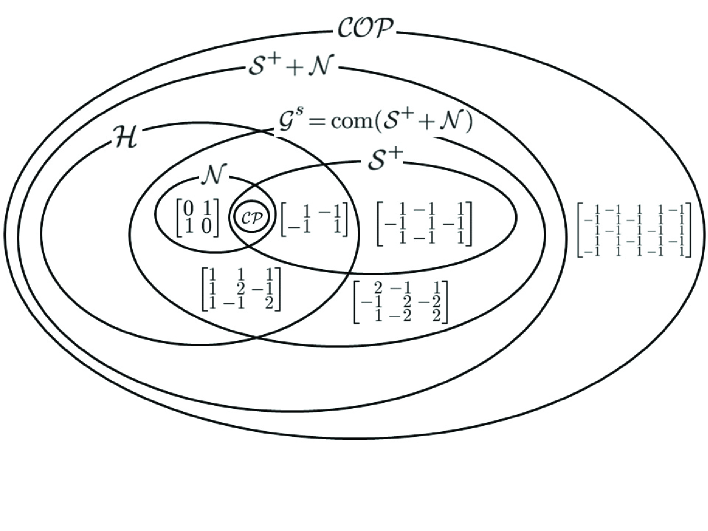
Figure 1: Examples of inclusion relations among the subcones of $\mathcal{S}_{n}^{+}+\mathcal{N}_{n}$ I

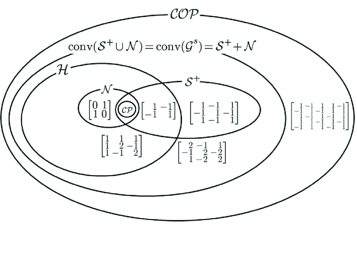
Figure 2: Examples of inclusion relations among the subcones of $\mathcal{S}_{n}^{+}+\mathcal{N}_{n}$ II

At present, it is not clear whether the set $\mathcal{G}_{n}={\rm com}\,(\mathcal{S}_{n}^{+},\mathcal{N}_{n})$ is convex or not. As we will mention on page 3, our numerical results suggest that the set might be not convex.

Before closing this discussion, we should point out another interesting subset of $\mathcal{S}_{n}^{+}+\mathcal{N}_{n}$ proposed by Bomze and Eichfelder [10]. Suppose that a given matrix $A\in\mathcal{S}_{n}$ can be decomposed as (6), and define the diagonal matrix $\Lambda_{+}$ by $[\Lambda_{+}]_{ii}=\max\{0,\lambda_{i}\}$. Let $A_{+}:=P\Lambda_{+}P^{T}$ and $A_{-}:=A_{+}-A$. Then, we can easily see that $A_{+}$ and $A_{-}$ are positive semidefinite. Using this decomposition $A=A_{+}-A_{-}$, Bomze and Eichfelder derived the following LP-based sufficient condition for $A\in\mathcal{S}_{n}^{+}+\mathcal{N}_{n}$ in [10].

Theorem 2.4 (Theorem 2.6 of [10]).

Let $x\in\mathbb{R}_{n}^{+}$ be such that $A_{+}x$ has only positive coordinates. If

$$(x^{T}A_{+}x)(A_{-})_{ii}\leq[(A_{+}x)_{i}]^{2}\ (i=1,2,\ldots,n)$$

then $A\in\mathcal{COP}_{n}$.

Consider the following LP with $O(n)$ variables and $O(n)$ constraints,

$$\inf\{f^{T}x\mid A_{+}x\geq e,\ x\in\mathbb{R}_{n}^{+}\}$$ (17)

where $f$ is an arbitrary vector and $e$ denotes the vector of all ones. Define the set,

$$\mathcal{L}_{n}:=\{A\in\mathcal{S}_{n}\mid(x^{T}A_{+}x)(A_{-})_{ii}\leq[(A_{+}x)_{i}]^{2}\ (i=1,2,\ldots,n)\ \mbox{for some feasible solution $x$ of (\ref{eq:LP_Bomze})}\}.$$

Then Theorem 2.4 ensures that $\mathcal{L}_{n}\subseteq\mathcal{COP}_{n}$. The following proposition gives a characterization when the feasible set of the LP of (17) is empty.

Proposition 2.5 (Proposition 2.7 of [10]).

The condition ${\rm ker}A_{+}\cap\{x\in\mathbb{R}_{n}^{+}\mid e^{T}x=1\}\neq\emptyset$ is equivalent to $\{x\in\mathbb{R}_{n}^{+}\mid A_{+}x\geq e\}=\emptyset$.

Consider the matrix,

$$A=\left[\begin{array}[]{rr}1&-1\\ -1&1\\ \end{array}\right]\in\mathcal{S}_{2}^{+}.$$

Thus, $A_{+}=A$, and the set ${\rm ker}A_{+}\cap\{x\in\mathbb{R}_{n}^{+}\mid e^{T}x=1\}\neq\emptyset$. Proposition 2.5 ensures that $A\not\in\mathcal{L}_{2}$, and hence, $\mathcal{S}_{n}^{+}\not\subseteq\mathcal{L}_{n}$ for $n\geq 2$, similarly to the set $\mathcal{H}_{n}$ for $n\geq 3$ (see Theorem 2.1).

3 Semidefinite bases

In this section, we improve the subcone $\mathcal{G}_{n}$ in terms of P2. For a given matrix $A$ of (6), the linear optimization problem $\mbox{(LP)}_{P,\Lambda}$ in (10) can be solved in order to find a nonnegative matrix that is a linear combination

$$\sum_{i=1}^{n}\omega_{i}p_{i}p_{i}^{T}$$

of $n$ linearly independent positive semidefinite matrices $p_{i}p_{i}^{T}\in\mathcal{S}_{n}^{+}\ (i=1,2,\ldots,n)$. This is done by decomposing $A\in\mathcal{S}_{n}$ into two parts:

$$A=\sum_{i=1}^{n}(\lambda_{i}-\omega_{i})p_{i}p_{i}^{T}+\sum_{i=1}^{n}\omega_{i}p_{i}p_{i}^{T}$$ (18)

such that the first part

$$\sum_{i=1}^{n}(\lambda_{i}-\omega_{i})p_{i}p_{i}^{T}$$

is positive semidefinite. Since $p_{i}p_{i}^{T}\in\mathcal{S}_{n}^{+}\ (i=1,2,\ldots,n)$ are only $n$ linearly independent matrices in $n(n+1)/2$ dimensional space $\mathcal{S}_{n}$, the intersection of the set of linear combinations of $p_{i}p_{i}^{T}$ and the nonnegative cone $\mathcal{N}_{n}$ may not have a nonzero volume even if it is nonempty. On the other hand, if we have a set of positive semidefinite matrices $p_{i}p_{i}^{T}\in\mathcal{S}_{n}^{+}\ (i=1,2,\ldots,n(n+1)/2)$ that gives a basis of $\mathcal{S}_{n}$, then the corresponding intersection becomes the nonnegative cone $\mathcal{N}_{n}$ itself, and we may expect a greater chance of finding a nonnegative matrix by enlarging the feasible region of $\mbox{(LP)}_{P,\Lambda}$. In fact, we can easily find a basis of $\mathcal{S}_{n}$ consisting of $n(n+1)/2$ semidefinite matrices from $n$ given orthogonal vectors $p_{i}\in\mathbb{R}^{n}\ (i=1,2,\ldots,n)$ based on the following result from [18].

Proposition 3.1 (Lemma 6.2 of [18]).

Let $v_{i}\in\mathbb{R}^{n}(i=1,2,\ldots,n)$ be $n$-dimensional linear independent vectors. Then the set $\mathcal{V}:=\{(v_{i}+v_{j})(v_{i}+v_{j})^{T}\mid 1\leq i\leq j\leq n\}$ is a set of $n(n+1)/2$ linearly independent positive semidefinite matrices. Therefore, the set $\mathcal{V}$ gives a basis of the set $\mathcal{S}_{n}$ of $n\times n$ symmetric matrices.

The above proposition ensures that the following set $\mathcal{B}_{+}(p_{1},p_{2},\ldots,p_{n})$ is a basis of $n\times n$ symmetric matrices.

Definition 3.2 (Semidefinite basis type I).

For a given set of $n$-dimensional orthogonal vectors $p_{i}\in\mathbb{R}^{n}(i=1,2,\ldots,n)$, define the map $\Pi_{+}:\mathbb{R}^{n}\times\mathbb{R}^{n}\rightarrow\mathcal{S}_{n}^{+}$ by

$$\Pi_{+}(p_{i},p_{j}):=\frac{1}{4}(p_{i}+p_{j})(p_{i}+p_{j})^{T}.$$ (19)

We call the set

$$\mathcal{B}_{+}(p_{1},p_{2},\ldots,p_{n}):=\{\Pi_{+}(p_{i},p_{j})\mid 1\leq i\leq j\leq n\}$$ (20)

a semidefinite basis type I induced by $p_{i}\in\mathbb{R}^{n}(i=1,2,\ldots,n)$.

A variant of the semidefinite basis type I is as follows. Noting that the equivalence

$$\Pi_{+}(p_{i},p_{j})=\frac{1}{2}p_{i}p_{i}^{T}+\frac{1}{2}p_{j}p_{j}^{T}-\Pi_{-}(p_{i},p_{j})$$

holds for any $i\neq j$, we see that $\mathcal{B}_{-}(p_{1},p_{2},\ldots,p_{n})$ is also a basis of $n\times n$ symmetric matrices.

Definition 3.3 (Semidefinite basis type II).

For a given set of $n$-dimensional orthogonal vectors $p_{i}\in\mathbb{R}^{n}(i=1,2,\ldots,n)$, define the map $\Pi_{+}:\mathbb{R}^{n}\times\mathbb{R}^{n}\rightarrow\mathcal{S}_{n}^{+}$ by

$$\Pi_{-}(p_{i},p_{j}):=\frac{1}{4}(p_{i}-p_{j})(p_{i}-p_{j})^{T}.$$ (21)

We call the set

$$\mathcal{B}_{-}(p_{1},p_{2},\cdots,p_{n}):=\{\Pi_{+}(p_{i},p_{i})\mid 1\leq i\leq n\}\cup\{\Pi_{-}(p_{i},p_{j})\mid 1\leq i<j\leq n\}$$ (22)

a semidefinite basis type II induced by $p_{i}\in\mathbb{R}^{n}(i=1,2,\ldots,n)$.

Using the map $\Pi_{+}$ in (19), the linear optimization problem $\mbox{(LP)}_{P,\Lambda}$ in (10) can be equivalently written as

$$\mbox{(LP)}_{P,\Lambda}\ \left|\begin{array}[]{lll}\mbox{Maximize}&\alpha&\\ \mbox{subject to}&\omega_{ii}^{+}\leq\lambda_{i}&(i=1,2,\ldots,n)\\ &\displaystyle{\left[\sum_{k=1}^{n}\omega_{kk}^{+}\Pi_{+}(p_{k},p_{k})\right]_{ij}\geq\alpha}&(1\leq i\leq j\leq n).\end{array}\right.$$

The problem $\mbox{(LP)}_{P,\Lambda}$ is based on the decomposition (18). Starting with (18), the matrix $A$ can be decomposed using $\Pi_{+}(p_{i},p_{j})$ in (19) and $\Pi_{-}(p_{i},p_{j})$ in (21) as

$$A = \sum_{i=1}^{n}(\lambda_{i}-\omega^{+}_{ii})\Pi_{+}(p_{i},p_{i})+\sum_{i=1}^{n}\omega^{+}_{ii}\Pi_{+}(p_{i},p_{i})$$ (24)

$$= \sum_{i=1}^{n}(\lambda_{i}-\omega^{+}_{ii})\Pi_{+}(p_{i},p_{i})+\sum_{i=1}^{n}\omega^{+}_{ii}\Pi_{+}(p_{i},p_{i})$$

$$\ \ \ +\sum_{1\leq i<j\leq n}(-\omega^{+}_{ij})\Pi_{+}(p_{i},p_{j})+\sum_{1\leq i<j\leq n}\omega^{+}_{ij}\Pi_{+}(p_{i},p_{j})$$

$$= \sum_{i=1}^{n}(\lambda_{i}-\omega^{+}_{ii})\Pi_{+}(p_{i},p_{i})+\sum_{i=1}^{n}\omega^{+}_{ii}\Pi_{+}(p_{i},p_{i})$$

$$\ \ \ +\sum_{1\leq i<j\leq n}(-\omega^{+}_{ij})\Pi_{+}(p_{i},p_{j})+\sum_{1\leq i<j\leq n}\omega^{+}_{ij}\Pi_{+}(p_{i},p_{j})$$

$$\ \ \ +\sum_{1\leq i<j\leq n}(-\omega^{-}_{ij})\Pi_{-}(p_{i},p_{j})+\sum_{1\leq i<j\leq n}\omega^{-}_{ij}\Pi_{-}(p_{i},p_{j}).$$

On the basis of the decomposition (24) and (24), we devise the following two linear optimization problems as extensions of $\mbox{(LP)}_{P,\Lambda}$:

$$\ \mbox{(LP)}_{P,\Lambda}^{+}\ \left|\begin{array}[]{lll}\mbox{Maximize}&\alpha&\\ \mbox{subject to}&\omega^{+}_{ii}\leq\lambda_{i}&(i=1,2,\ldots,n)\\ &\omega^{+}_{ij}\leq 0&(1\leq i<j\leq n)\\ &\displaystyle{\left[\sum_{1\leq k\leq l\leq n}\omega^{+}_{kl}\Pi_{+}(p_{k},p_{l})\right]_{ij}\geq\alpha}&(1\leq i\leq j\leq n)\end{array}\right.$$ (29)

$$\mbox{(LP)}_{P,\Lambda}^{\pm}\ \left|\begin{array}[]{lll}\mbox{Maximize}&\alpha&\\ \mbox{subject to}&\omega^{+}_{ii}\leq\lambda_{i}&(i=1,2,\ldots,n)\\ &\omega^{+}_{ij}\leq 0,\ \omega^{-}_{ij}\leq 0&(1\leq i<j\leq n)\\ &\displaystyle{\left[\sum_{1\leq k\leq l\leq n}\omega^{+}_{kl}\Pi_{+}(p_{k},p_{l})+\sum_{1\leq k<l\leq n}\omega^{-}_{kl}\Pi_{-}(p_{k},p_{l})\right]_{ij}\geq\alpha}&(1\leq i\leq j\leq n)\end{array}\right.$$ (34)

(35)

Problem $\mbox{(LP)}_{P,\Lambda}^{+}$ has $n(n+1)/2+1$ variables and $n(n+1)$ constraints, and problem $\mbox{(LP)}_{P,\Lambda}^{\pm}$ has $n^{2}+1$ variables and $n(3n+1)/2$ constraints (see Table 1). Since $[P\Omega P^{T}]_{ij}$ in (10) is given by $\left[\sum_{k=1}^{n}\omega_{kk}\Pi_{+}(p_{k},p_{k})\right]_{ij}$, we can prove that both linear optimization problems $\mbox{(LP)}_{P,\Lambda}^{+}$ and $\mbox{(LP)}_{P,\Lambda}^{\pm}$ are feasible and bounded by making arguments similar to the one for $\mbox{(LP)}_{P,\Lambda}$ on page 2. Thus, $\mbox{(LP)}_{P,\Lambda}^{+}$ and $\mbox{(LP)}_{P,\Lambda}^{\pm}$ have optimal solutions with corresponding optimal values $\alpha_{*}^{+}(P,\Lambda)$ and $\alpha_{*}^{\pm}(P,\Lambda)$.

If the optimal value $\alpha_{*}^{+}(P,\Lambda)$ of $\mbox{(LP)}_{P,\Lambda}^{+}$ is nonnegative, then, by rearranging (24), the optimal solution $\omega^{+*}_{ij}\ (1\leq i\leq j\leq n)$ can be made to give the following decomposition:

$$A=\left[\sum_{i=1}^{n}(\lambda_{i}-\omega^{+*}_{ii})\Pi_{+}(p_{i},p_{i})+\sum_{1\leq i<j\leq n}(-\omega^{+*}_{ij})\Pi_{+}(p_{i},p_{j})\right]+\left[\sum_{1\leq i\leq j\leq n}\omega^{+*}_{ij}\Pi_{+}(p_{i},p_{j})\right]\in\mathcal{S}_{n}^{+}+\mathcal{N}_{n}.$$

In the same way, if the optimal value $\alpha_{*}^{\pm}(P,\Lambda)$ of $\mbox{(LP)}_{P,\Lambda}^{\pm}$ is nonnegative, then, by rearranging (24), the optimal solution $\omega^{+*}_{ij}\ (1\leq i\leq j\leq n)$, $\omega^{-*}_{ij}\ (1\leq i<j\leq n)$ can be made to give the following decomposition:

$$A = \left[\sum_{i=1}^{n}(\lambda_{i}-\omega^{+*}_{ii})\Pi_{+}(p_{i},p_{i})+\sum_{1\leq i<j\leq n}(-\omega^{+*}_{ij})\Pi_{+}(p_{i},p_{j})+\sum_{1\leq i<j\leq n}(-\omega^{-*}_{ij})\Pi_{-}(p_{i},p_{j})\right]$$

$$\ \ \ \ \ +\left[\sum_{1\leq i\leq j\leq n}\omega^{+*}_{ij}\Pi_{+}(p_{i},p_{j})+\sum_{1\leq i<j\leq n}\omega^{-*}_{ij}\Pi_{-}(p_{i},p_{j})\right]\ \ \in\mathcal{S}_{n}^{+}+\mathcal{N}_{n}.$$

On the basis of the above observations, we can define new subcones of $\mathcal{S}_{n}^{+}+\mathcal{N}_{n}$ in a similar manner as (11) and (13).

For a given $A\in\mathcal{S}_{n}$, define the following four sets of pairs of matrices

$$\begin{array}[]{rcl}\mathcal{PL}_{\mathcal{F}_{n}^{+}}(A)&:=&\{(P,\Lambda)\in{\cal O}_{n}\times{\cal D}_{n}\mid\mbox{$P$ and $\Lambda$ satisfy (\ref{eq:diagonalization}) and $\alpha_{*}^{+}(P,\Lambda)\geq 0$}\}\\ \mathcal{PL}_{\mathcal{F}_{n}^{\pm}}(A)&:=&\{(P,\Lambda)\in{\cal O}_{n}\times{\cal D}_{n}\mid\mbox{$P$ and $\Lambda$ satisfy (\ref{eq:diagonalization}) and $\alpha_{*}^{\pm}(P,\Lambda)\geq 0$}\}\\ \mathcal{PL}_{\widehat{\mathcal{F}_{n}^{+}}}(A)&:=&\{(P,\Lambda)\in\mathbb{R}^{n\times n}\times{\cal D}_{n}\mid\mbox{$P$ and $\Lambda$ satisfy (\ref{eq:diagonalization}) and $\alpha_{*}^{+}(P,\Lambda)\geq 0$}\}\\ \mathcal{PL}_{\widehat{\mathcal{F}_{n}^{\pm}}}(A)&:=&\{(P,\Lambda)\in\mathbb{R}^{n\times n}\times{\cal D}_{n}\mid\mbox{$P$ and $\Lambda$ satisfy (\ref{eq:diagonalization}) and $\alpha_{*}^{\pm}(P,\Lambda)\geq 0$}\}\end{array}$$ (36)

where $\alpha_{*}^{+}(P,\Lambda)$ and $\alpha_{*}^{\pm}(P,\Lambda)$ are optimal values of $\mbox{(LP)}_{P,\Lambda}^{+}$ and $\mbox{(LP)}_{P,\Lambda}^{\pm}$, respectively. Using the above sets, we define new subcones of $\mathcal{S}_{n}^{n}+\mathcal{N}_{n}$ as follows:

$$\begin{array}[]{rcl}\mathcal{F}_{n}^{+}&:=&\{A\in\mathcal{S}_{n}\mid\mathcal{PL}_{\mathcal{F}_{n}^{+}}(A)\neq\emptyset\},\\ \mathcal{F}_{n}^{\pm}&:=&\{A\in\mathcal{S}_{n}\mid\mathcal{PL}_{\mathcal{F}_{n}^{\pm}}(A)\neq\emptyset\},\\ \widehat{\mathcal{F}_{n}^{+}}&:=&\{A\in\mathcal{S}_{n}\mid\mathcal{PL}_{\widehat{\mathcal{F}_{n}^{+}}}(A)\neq\emptyset\},\\ \widehat{\mathcal{F}_{n}^{\pm}}&:=&\{A\in\mathcal{S}_{n}\mid\mathcal{PL}_{\widehat{\mathcal{F}_{n}^{\pm}}}(A)\neq\emptyset\}.\end{array}$$ (37)

From the construction of problems $\mbox{(LP)}_{P,\Lambda}$, $\mbox{(LP)}_{P,\Lambda}^{+}$ and $\mbox{(LP)}_{P,\Lambda}^{\pm}$, and the definitions (36) and (37), we can easily see that

$$\mathcal{G}_{n}\subseteq\mathcal{F}_{n}^{+}\subseteq\mathcal{F}_{n}^{\pm},\ \ \ \ \ \widehat{\mathcal{G}_{n}}\subseteq\widehat{\mathcal{F}_{n}^{+}}\subseteq\widehat{\mathcal{F}_{n}^{\pm}},\ \ \ \ \ \mathcal{F}_{n}^{+}\subseteq\widehat{\mathcal{F}_{n}^{+}},\ \ \ \ \ \mathcal{F}_{n}^{\pm}\subseteq\widehat{\mathcal{F}_{n}^{\pm}}$$

hold. The corollary below follows from (iv)-(vi) of Theorem 2.3 and the above inclusions.

Corollary 3.4.

(i)

$$\begin{array}[]{ccccccccc}\mathcal{S}_{n}^{+}\cup\mathcal{N}_{n}&\subseteq&\mathcal{G}_{n}=\mbox{\rm com}(\mathcal{S}_{n}^{+}+\mathcal{N}_{n})&\subseteq&\widehat{\mathcal{G}_{n}}&\subseteq&\mathcal{S}_{n}^{+}+\mathcal{N}_{n}\\ &&\rotatebox{270.0}{$\subseteq$}&&\rotatebox{270.0}{$\subseteq$}&&\\ \mathcal{S}_{n}^{+}\cup\mathcal{N}_{n}&\subseteq&\mathcal{F}_{n}^{+}&\subseteq&\widehat{\mathcal{F}_{n}^{+}}&\subseteq&\mathcal{S}_{n}^{+}+\mathcal{N}_{n}\\ &&\rotatebox{270.0}{$\subseteq$}&&\rotatebox{270.0}{$\subseteq$}&&\\ \mathcal{S}_{n}^{+}\cup\mathcal{N}_{n}&\subseteq&\mathcal{F}_{n}^{\pm}&\subseteq&\widehat{\mathcal{F}_{n}^{\pm}}&\subseteq&\mathcal{S}_{n}^{+}+\mathcal{N}_{n}\\ \end{array}$$

(ii)

If $n=2$, then each of the sets $\mathcal{F}_{n}^{+}$, $\widehat{\mathcal{F}_{n}^{+}}$, $\mathcal{F}_{n}^{\pm}$, and $\widehat{\mathcal{F}_{n}^{\pm}}$ coincides with $\mathcal{S}_{n}^{+}+\mathcal{N}_{n}$.

(iii)

The convex hull of each of the sets $\mathcal{F}_{n}^{+}$, $\widehat{\mathcal{F}_{n}^{+}}$, $\mathcal{F}_{n}^{\pm}$, and $\widehat{\mathcal{F}_{n}^{\pm}}$ is $\mathcal{S}_{n}^{+}+\mathcal{N}_{n}$.

The following table summarizes the sizes of LPs (10), (29), and (35) that we have to solve in order to identify, respectively, $(P,\Lambda)\in\mathcal{PL}_{\mathcal{G}_{n}}(A)$ (or $(P,\Lambda)\in\mathcal{PL}_{\widehat{\mathcal{G}_{n}}}(A)$), $(P,\Lambda)\in\mathcal{PL}_{\mathcal{F}_{n}^{+}}(A)$ (or $(P,\Lambda)\in\mathcal{PL}_{\widehat{\mathcal{F}_{n}^{+}}}(A)$), and $(P,\Lambda)\in\mathcal{PL}_{\mathcal{F}_{n}^{\pm}}$ (or $(P,\Lambda)\in\mathcal{PL}_{\widehat{\mathcal{F}_{n}^{\pm}}}(A)$).

Table 1: Sizes of LPs for identification

Identification	$(P,\Lambda)\in\mathcal{PL}_{\mathcal{G}_{n}}(A)$	$(P,\Lambda)\in\mathcal{PL}_{\mathcal{F}_{n}^{+}}(A)$	$(P,\Lambda)\in\mathcal{PL}_{\mathcal{F}_{n}^{\pm}}$
	(or $(P,\Lambda)\in\mathcal{PL}_{\widehat{\mathcal{G}_{n}}}(A)$)	(or $(P,\Lambda)\in\mathcal{PL}_{\widehat{\mathcal{F}_{n}^{+}}}(A)$)	(or $(P,\Lambda)\in\mathcal{PL}_{\widehat{\mathcal{F}_{n}^{\pm}}}(A)$)
# of variables	$n+1$	$n(n+1)/2+1$	$n^{2}+1$
# of constraints	$n(n+3)/2$	$n(n+1)$	$n(3n+1)/2$

4 Identification of $A\in\mathcal{S}_{n}^{+}+\mathcal{N}_{n}$

In this section, we investigate the effect of using the sets $\mathcal{G}_{n}$, $\mathcal{F}_{n}^{+}$ and $\mathcal{F}_{n}^{\pm}$ for identification of the fact $A\in\mathcal{S}_{n}^{+}+\mathcal{N}_{n}$.

We generated random instances of $A\in\mathcal{S}_{n}^{+}+\mathcal{N}_{n}$ by using the method described in Section 2 of [10]. For an $n\times n$ matrix $B$ with entries independently drawn from a standard normal distribution, we obtained a random positive semidefinite matrix $S=BB^{T}$. An $n\times n$ random nonnegative matrix $N$ was constructed using $N=C-c_{\min}I_{n}$ with $C=F+F^{T}$ for a random matrix $F$ with entries uniformly distributed in $[0,1]$ and $c_{\min}$ being the minimal diagonal entry of $C$. We set $A=S+N\in\mathcal{S}_{n}^{+}+\mathcal{N}_{n}$. The construction was designed so as to maintain the nonnegativity of $N$ while increasing the chance that $S+N$ would be indefinite and thereby avoid instances that are too easy.

For each instance $A\in\mathcal{S}^{+}_{n}+\mathcal{N}_{n}$, we used the MATLAB command “$[P,\Lambda]=\mbox{eig}(A)$” and obtained $(P,\Lambda)\in\mathcal{O}_{n}\times\mathcal{D}_{n}$. We checked whether $(P,\lambda)\in\mathcal{PL}_{\mathcal{G}_{n}}$ ($(P,L)\in\mathcal{PL}_{\mathcal{F}_{n}^{+}}$ and $(P,L)\in\mathcal{PL}_{\mathcal{F}_{n}^{\pm}}$) by solving ($\mbox{LP})_{P,\Lambda}$ in (10) ( ($\mbox{LP})_{P,\Lambda}^{+}$ in (29) and ($\mbox{LP})_{P,\Lambda}^{\pm}$ in (35)) and if it held, we identified that $A\in\mathcal{G}_{n}$ ($A\in\mathcal{F}_{n}^{+}$ and $A\in\mathcal{F}_{n}^{\pm}$).

Table 2 shows the number of matrices (denoted by “#$A$”) that were identified as $A\in\mathcal{H}_{n}$ ($A\in\mathcal{G}_{n}^{+}$, $A\in\mathcal{F}_{n}^{+}$, $A\in\mathcal{F}_{n}^{\pm}$ and $A\in\mathcal{S}_{n}^{+}+\mathcal{N}_{n}$) and the average CPU time (denoted by “A.t.(s)”), where $1000$ matrices were generated for each $n$. We used a 3.07GHz Core i7 machine with 12 GB of RAM and Gurobi 6.5 for solving LPs. Note that we performed the last identification $A\in\mathcal{S}_{n}^{+}+\mathcal{N}_{n}$ as a reference, while we used SeDuMi 1.3 with MATLAB R2015a for solving the semidefinite program (3). The table yields the following observations:

• All of the matrices were identified as $A\in\mathcal{S}^{+}_{n}+\mathcal{N}_{n}$ by checking $(P,L)\in\mathcal{PL}_{\mathcal{F}_{n}^{\pm}}$. The result is comparable to the one in Section 2 of [10]. The average CPU time for checking $(P,L)\in\mathcal{PL}_{\mathcal{F}_{n}^{\pm}}$ is faster than the one for solving the semidefinite program (3) when $n\geq 20$.

• For any $n$, the number of identified matrices increases in the order of the set inclusion relation: $\mathcal{G}_{n}\subseteq\mathcal{F}_{n}^{+}\subseteq\mathcal{F}_{n}^{\pm}$, while the result for $\mathcal{H}_{n}\not\subseteq\mathcal{G}_{n}$ is better than the one for $\mathcal{G}_{n}$ when $n=10$.

• For the sets $\mathcal{H}_{n}$, $\mathcal{G}_{n}$ and $\mathcal{F}_{n}^{+}$, the number of identified matrices decreases as the size of $n$ increases.

Table 2: Results of identification of $A\in\mathcal{S}^{+}_{n}+\mathcal{N}_{n}$: $1000$ matrices were generated for each $n$.

	$\mathcal{H}_{n}$		$\mathcal{G}_{n}$		$\mathcal{F}_{n}^{+}$		$\mathcal{F}_{n}^{\pm}$		$\mathcal{S}_{n}^{+}+\mathcal{N}_{n}$
$n$	#$A$	A.t.(s)	#$A$	A.t.(s)	#$A$	A.t.(s)	#$A$	A.t.(s)	#$A$	A.t.(s)
10	791	0.001	247	0.005	856	0.008	1000	0.011	1000	0.824
20	16	0.001	20	0.013	719	0.121	1000	0.222	1000	9.282
50	0	0.003	0	2.374	440	22.346	1000	50.092	1000	1285.981

5 LP-based algorithms for testing $A\in\mathcal{COP}_{n}$

In this section, we investigate the effect of using the sets $\mathcal{F}_{n}^{+}$, $\widehat{\mathcal{F}_{n}^{+}}$, $\mathcal{F}_{n}^{\pm}$ and $\widehat{\mathcal{F}_{n}^{\pm}}$ for testing whether a given matrix $A$ is copositive by using Sponsel, Bundfuss, and Dür’s algorithm [36].

5.1 Outline of the algorithms

By defining the standard simplex $\Delta^{S}$ by $\Delta^{S}=\{x\in\mathbb{R}^{n}_{+}\mid e^{T}x=1\}$, we can see that a given $n\times n$ symmetric matrix $A$ is copositive if and only if

$$x^{T}Ax\geq 0\ \mbox{ for all }\ x\in\Delta^{S}$$

(see Lemma 1 of [12]). For an arbitrary simplex $\Delta$, a family of simplices $\mathcal{P}=\{\Delta^{1},\ldots,\Delta^{m}\}$ is called a simplicial partition of $\Delta$ if it satisfies

$$\Delta=\bigcup_{i=1}^{m}\Delta^{i}\ \mbox{and}\ \mbox{int}(\Delta^{i})\cap\mbox{int}(\Delta^{j})=\emptyset\ \mbox{for all}\ i\neq j.$$

Such a partition can be generated by successively bisecting simplices in the partition. For a given simplex $\Delta=\mbox{conv}\{v_{1},\ldots,v_{n}\}$, consider the midpoint $v_{n+1}=\frac{1}{2}(v_{i}+v_{j})$ of the edge $[v_{i},v_{j}]$. Then the subdivision $\Delta^{1}=\{v_{1},\ldots,v_{i-1},v_{n+1},v_{i+1},\ldots,v_{n}\}$ and $\Delta^{2}=\{v_{1},\ldots,v_{j-1},v_{n+1},v_{j+1},\ldots,v_{n}\}$ of $\Delta$ satisfies the above conditions for simplicial partitions. See [27] for a detailed description of simplicial partitions.

Denote the set of vertices of partition $\mathcal{P}$ by

$$V(\mathcal{P})=\{v\mid\mbox{$v$ is a vertex of some $\Delta\in\mathcal{P}$}\}.$$

Each simplex $\Delta$ is determined by its vertices and can be represented by a matrix $V_{\Delta}$ whose columns are these vertices. Note that $V_{\Delta}$ is nonsingular and unique up to a permutation of its columns, which does not affect the argument [36]. Define the set of all matrices corresponding to simplices in partition $\mathcal{P}$ as

$$M(\mathcal{P})=\{V_{\Delta}:\Delta\in\mathcal{P}\}.$$

The “fineness” of a partition $\mathcal{P}$ is quantified by the maximum diameter of a simplex in $\mathcal{P}$, denoted by

$$\delta(\mathcal{P})=\max_{\Delta\in\mathcal{P}}\max_{u,v\in\Delta}||u-v||.$$ (38)

The above notation was used to show the following necessary and sufficient conditions for copositivity in [36]. The first theorem gives a sufficient condition for copositivity.

Theorem 5.1 (Theorem 2.1 of [36]).

If $A\in\mathcal{S}_{n}$ satisfies

$$V^{T}AV\in\mathcal{COP}_{n}\ \mbox{for all}\ V\in M(\mathcal{P})$$

then $A$ is copositive. Hence, for any $\mathcal{M}_{n}\subseteq\mathcal{COP}_{n}$, if $A\in\mathcal{S}_{n}$ satisfies

$$V^{T}AV\in\mathcal{M}_{n}\ \mbox{for all}\ V\in M(\mathcal{P}),$$

then $A$ is also copositive.

The above theorem implies that by choosing $\mathcal{M}_{n}=\mathcal{N}_{n}$ (see (2)), $A$ is copositive if $V^{T}_{\Delta}AV_{\Delta}\in\mathcal{N}_{n}$ holds for any $\Delta\in\mathcal{P}$.

Theorem 5.2 (Theorem 2.2 of [36]).

Let $A\in\mathcal{S}_{n}$ be strictly copositive, i.e., $A\in{\rm int}\,(\mathcal{COP}_{n})$. Then there exists $\varepsilon>0$ such that for all partitions $\mathcal{P}$ of $\Delta^{S}$ with $\delta(\mathcal{P})<\varepsilon$, we have

$$V^{T}AV\in\mathcal{N}_{n}\ \mbox{for all}\ V\in M(\mathcal{P}).$$

The above theorem ensures that if $A$ is strictly copositive (i.e., $A\in{\rm int}\,(\mathcal{COP}_{n})$), the copositivity of $A$ (i.e., $A\in\mathcal{COP}_{n}$) can be detected in finitely many iterations of an algorithm employing a subdivision rule with $\delta(\mathcal{P})\rightarrow 0$. A similar result can be obtained for the case $A\not\in\mathcal{COP}_{n}$, as follows.

Lemma 5.3 (Lemma 2.3 of [36]).

The following two statements are equivalent.

1. $A\notin\mathcal{COP}_{n}$

2. There is an $\varepsilon>0$ such that for any partition $\mathcal{P}$ with $\delta(\mathcal{P})<\varepsilon$, there exists a vertex $v\in V(\mathcal{P})$ such that $v^{T}Av<0$.

The following algorithm, from [36], is based on the above three results.

Algorithm 1 Sponsel, Bundfuss, and Dür’s algorithm to test copositivity

0:  $A\in\mathcal{S}_{n},\mathcal{M}_{n}\subseteq\mathcal{COP}_{n}$

0:  “$A$ is copositive” or “$A$ is not copositive”

1:  $\mathcal{P}\leftarrow\{\Delta^{S}\}$;

2:  while $\mathcal{P}\neq\emptyset$ do

3:     Choose $\Delta\in\mathcal{P}$;

4:     if $v^{T}Av<0$ for some $v\in V(\{\Delta\})$: then

5:        return “$A$ is not copositive”;

6:     end if

7:     if we identify $V_{\Delta}^{T}AV_{\Delta}\in\mathcal{M}_{n}$ then

8:        $\mathcal{P}\leftarrow\mathcal{P}\setminus\{\Delta\}$;

9:     else

10:        Partition $\Delta$ into $\Delta=\Delta^{1}\cup\Delta^{2}$;

11:        $\mathcal{P}\leftarrow\mathcal{P}\setminus\{\Delta\}\cup\{\Delta^{1},\Delta^{2}\}$;

12:     end if

13:  end while

14:  Return “$A$ is copositive”;

As we have already observed, Theorem 5.2 and Lemma 5.3 imply the following corollary.

Corollary 5.4.

1. If $A$ is strictly copositive, i.e., $A\in{\rm int}\,(\mathcal{COP}_{n})$, then Algorithm 1 terminates finitely, returning “A is copositive.”

2. If $A$ is not copositive, i.e., $A\not\in\mathcal{COP}_{n}$, then Algorithm 1 terminates finitely, returning “A is not copositive.”

In this section, we investigate the effect of using the sets $\mathcal{H}_{n}$ from (5), $\mathcal{G}_{n}$ from (11), and $\mathcal{F}_{n}^{+}$ and $\mathcal{F}_{n}^{\pm}$ from (37) as the set $\mathcal{M}_{n}$ in the above algorithm.

At Line 7, we can check whether $V_{\Delta}^{T}AV_{\Delta}\in\mathcal{M}_{n}$ directly in the case where $\mathcal{M}_{n}=\mathcal{H}_{n}$. In other cases, we diagonalize $V_{\Delta}^{T}AV_{\Delta}$ as $V_{\Delta}^{T}AV_{\Delta}=P\Lambda P^{T}$ and check whether $(P,\Lambda)\in\mathcal{PL}_{\mathcal{M}_{n}}(V_{\Delta}^{T}AV_{\Delta})$ according to definitions (12) or (36). If the associated LP has the nonnegative optimal value, then we identify $A\in\mathcal{M}_{n}$.

At Line 8, Algorithm 1 removes the simplex that was determined at Line 7 to be in no further need of exploration by Theorem 5.1. The accuracy and speed of the determination influence the total computational time and depend on the choice of the set $\mathcal{M}_{n}\subseteq\mathcal{COP}_{n}$.

Here, if we choose $\mathcal{M}_{n}=\mathcal{G}_{n}$ (respectively, $\mathcal{M}_{n}=\mathcal{F}_{n}^{+}$, $\mathcal{M}_{n}=\mathcal{F}_{n}^{\pm}$), we can improve Algorithm 1 by incorporating the set $\widehat{\mathcal{M}_{n}}=\widehat{\mathcal{G}_{n}}$ (respectively, $\widehat{\mathcal{M}_{n}}=\widehat{\mathcal{F}_{n}^{+}}$, $\widehat{\mathcal{M}_{n}}=\widehat{\mathcal{F}_{n}^{\pm}}$), as proposed in [37].

Algorithm 2 Improved version of Algorithm 1

0:  $A\in\mathcal{S}_{n},\mathcal{M}_{n}\subseteq\widehat{\mathcal{M}_{n}}\subseteq\mathcal{COP}_{n}$

0:  “$A$ is copositive” or “$A$ is not copositive”

1:  $\mathcal{P}\leftarrow\{\Delta^{S}\}$;

2:  while $\mathcal{P}\neq\emptyset$ do

3:     Choose $\Delta\in\mathcal{P}$;

4:     if $v^{T}Av<0$ for some $v\in V(\{\Delta\})$: then

5:        Return “$A$ is not copositive”;

6:     end if

7:     Let $P$ and $\Lambda$ be matrices satisfying $A=P\Lambda P^{T}$;

8:     if we identify $V_{\Delta}^{T}AV_{\Delta}\in\widehat{\mathcal{M}_{n}}$ by checking whether $(V_{\Delta}^{T}P,\Lambda)\in\mathcal{PL}_{\widehat{\mathcal{M}_{n}}}$ then

9:        $\mathcal{P}\leftarrow\mathcal{P}\setminus\{\Delta\}$;

10:     else

11:        Let $P$ and $\Lambda$ be matrices satisfying $V_{\Delta}^{T}AV_{\Delta}=P\Lambda P^{T}$;

12:        if we identify $V_{\Delta}^{T}AV_{\Delta}\in\mathcal{M}_{n}$ by checking whether $(P,\Lambda)\in\mathcal{PL}_{\mathcal{M}_{n}}$ then

13:           $\mathcal{P}\leftarrow\mathcal{P}\setminus\{\Delta\}$;

14:        else

15:           Partition $\Delta$ into $\Delta=\Delta^{1}\cup\Delta^{2}$, and set $\widehat{\Delta}\leftarrow\{\Delta^{1},\Delta^{2}$};

16:           for $p=1,2$ do

17:              Let $\Omega^{*}:={\rm Diag}\,(\omega^{*})$ where $\omega^{*}$ is an LP optimal solution obtained at Line 12;

18:              if we identify $V_{\Delta^{p}}^{T}AV_{\Delta^{p}}\in\widehat{\mathcal{M}_{n}}$ by checking whether $V_{\Delta^{p}}^{T}P\Omega^{*}P^{T}V_{\Delta^{p}}\in\mathcal{N}_{n}$ then

19:                 $\widehat{\Delta}\leftarrow\widehat{\Delta}\setminus\{\Delta^{p}\}$;

20:              end if

21:           end for

22:           $\mathcal{P}\leftarrow\mathcal{P}\setminus\{\Delta\}\cup\widehat{\Delta}$;

23:        end if

24:     end if

25:  end while

26:  return “$A$ is copositive”;

The details of the added steps are as follows. Suppose that we have a diagonalization of the form (6).

At Line 8, we need to solve an additional LP but do not need to diagonalize $V_{\Delta}^{T}AV_{\Delta}$. Let $P$ and $\Lambda$ be matrices satisfying (6). Then the matrix $V_{\Delta}^{T}P$ can be used to diagonalize $V_{\Delta}^{T}AV_{\Delta}$, i.e.,

$$V_{\Delta}^{T}AV_{\Delta}=V_{\Delta}^{T}(P\Lambda P^{T})V_{\Delta}=(V_{\Delta}^{T}P)\Lambda(V_{\Delta}^{T}P)^{T}$$

while $V_{\Delta}^{T}P\in\mathbb{R}^{n\times n}$ is not necessarily orthogonal. Thus, we can test whether $(V_{\Delta}^{T}P,\Lambda)\in\mathcal{PL}_{\widehat{\mathcal{M}_{n}}}$ by solving the corresponding LP according to the definitions (14) or (36). If $(V_{\Delta}^{T}P,\Lambda)\in\mathcal{PL}_{\widehat{\mathcal{M}_{n}}}$ holds, then we can identify $V_{\Delta}^{T}AV_{\Delta}\in\widehat{\mathcal{M}_{n}}$

If $(V_{\Delta}^{T}P,\Lambda)\not\in\mathcal{PL}_{\widehat{\mathcal{M}_{n}}}$ at Line 8, we proceed to the original step to identify whether $V_{\Delta}^{T}AV_{\Delta}\in\mathcal{M}_{n}$ at Line 12. Similarly to Line 7 of Algorithm 1, we diagonalize $V_{\Delta}^{T}AV_{\Delta}$ as $V_{\Delta}^{T}AV_{\Delta}=P\Lambda P^{T}$ with an orthogonal matrix $P$ and a diagonal matrix $\Lambda$. Then we check whether $(P,\Lambda)\in\mathcal{PL}_{\mathcal{M}_{n}}$ by solving the corresponding LP, and if $(P,\Lambda)\in\mathcal{PL}_{\mathcal{M}_{n}}$, we can identify $V_{\Delta}^{T}AV_{\Delta}\in\mathcal{M}_{n}$.

At Line 18, we don’t need to diagonalize $V_{\Delta^{p}}^{T}AV_{\Delta^{p}}$ or solve any more LPs. Let $\omega^{*}\in\mathbb{R}^{n}$ be an optimal solution of the corresponding LP obtained at Line 8 and let $\Omega^{*}:={\rm Diag}\,(\omega^{*})$. Then the feasibility of $\omega^{*}$ implies the positive semidefiniteness of the matrix $V_{\Delta^{p}}^{T}P(\Lambda-\Omega^{*})P^{T}V_{\Delta^{p}}$. Thus, if $V_{\Delta^{p}}^{T}P\Omega^{*}P^{T}V_{\Delta^{p}}\in\mathcal{N}_{n}$, we see that

$$V_{\Delta^{p}}^{T}AV_{\Delta^{p}}=V_{\Delta^{p}}^{T}P(\Lambda-\Omega^{*})P^{T}V_{\Delta^{p}}+V_{\Delta^{p}}^{T}P\Omega^{*}P^{T}V_{\Delta^{p}}\in\mathcal{S}_{n}^{+}+\mathcal{N}_{n}$$

and that $V_{\Delta^{p}}^{T}AV_{\Delta^{p}}\in\widehat{\mathcal{M}_{n}}$.

5.2 Numerical results

This subsection describes experiments for testing copositivity using $\mathcal{N}_{n}$,$\mathcal{H}_{n}$, $\mathcal{G}_{n}$, $\mathcal{F}_{n}^{+}$, $\widehat{\mathcal{F}_{n}^{+}}$, $\mathcal{F}_{n}^{\pm}$ or $\widehat{\mathcal{F}_{n}^{\pm}}$ as the set $\mathcal{M}_{n}$ in Algorithms 1 and 2. We implemented the following seven algorithms in MATLAB R2015a on a 3.07GHz Core i7 machine with 12 GB of RAM, using Gurobi 6.5 for solving LPs:

Algorithm 1.1:

Algorithm 1 with $\mathcal{M}_{n}=\mathcal{N}_{n}$.

Algorithm 1.2:

Algorithm 1 with $\mathcal{M}_{n}=\mathcal{H}_{n}$.

Algorithm 2.1:

Algorithm 2 with $\mathcal{M}_{n}=\mathcal{G}_{n}$ and $\widehat{\mathcal{M}_{n}}=\widehat{\mathcal{G}_{n}}$.

Algorithm 1.3:

Algorithm 1 with $\mathcal{M}_{n}=\mathcal{F}_{n}^{+}$.

Algorithm 2.2:

Algorithm 2 with $\mathcal{M}_{n}=\mathcal{F}_{n}^{+}$ and $\widehat{\mathcal{M}_{n}}=\widehat{\mathcal{F}_{n}^{+}}$.

Algorithm 2.3:

Algorithm 2 with $\mathcal{M}_{n}=\mathcal{F}_{n}^{\pm}$ and $\widehat{\mathcal{M}_{n}}=\widehat{\mathcal{F}_{n}^{\pm}}$.

Algorithm 1.4:

Algorithm 1 with $\mathcal{M}_{n}=\mathcal{S}_{n}^{+}+\mathcal{N}_{n}$.

As test instances, we used the two kinds of matrices arising from the maximum clique problem (Section 5.2.1) and from standard quadratic optimization problems (Section 5.2.2).

5.2.1 Results for the matrix arising from the maximum clique problem

In this subsection, we consider the matrix

$$B_{\gamma}:=\gamma(E-A_{G})-E$$ (39)

where $E\in\mathcal{S}_{n}$ is the matrix whose elements are all ones and the matrix $A_{G}\in\mathcal{S}_{n}$ is the adjacency matrix of a given undirected graph $G$ with $n$ nodes. The matrix $B_{\gamma}$ comes from the maximum clique problem. The maximum clique problem is to find a clique (complete subgraph) of maximum cardinality in $G$. It has been shown (in [15]) that the maximum cardinality, the so-called clique number $\omega(G)$, is equal to the optimal value of

$$\omega(G)=\min\{\gamma\in\mathbb{N}\mid B_{\gamma}\in\mathcal{COP}_{n}\}.$$

Thus, the clique number can be found by checking the copositivity of $B_{\gamma}$ for at most $\gamma=n,n-1,\ldots,1$.

Figure 3 shows the instances of $G$ that were used in [36]. We know the clique numbers of $G_{8}$ and $G_{12}$ are $\omega(G_{8})=3$ and $\omega(G_{12})=4$, respectively.

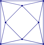
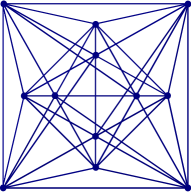
Figure 3: Graphs $G_{8}$ with $\omega(G_{8})=3$ (left) and $G_{12}$ with $\omega(G_{12})=4$ (right).

The aim of the implementation is to explore the differences in behavior when using $\mathcal{H}_{n}$, $\mathcal{G}_{n}$, $\mathcal{F}_{n}^{+}$, $\widehat{\mathcal{F}_{n}^{+}}$, $\mathcal{F}_{n}^{\pm}$ or $\widehat{\mathcal{F}_{n}^{\pm}}$ as the set $\mathcal{M}_{n}$ rather than to compute the clique number efficiently. Hence, the experiment examined $B_{\gamma}$ for various values of $\gamma$ at intervals of $0.1$ around the value $\omega(G)$ (see Tables 3 and 4 on page 3).

As already mentioned, $\alpha_{*}(P,\Lambda)<0$ ($\alpha^{+}_{*}(P,\Lambda)<0$ and $\alpha^{\pm}_{*}(P,\Lambda)<0$) with a specific $P$ does not necessarily guarantee that $A\not\in\mathcal{G}_{n}$ or $A\not\in\widehat{\mathcal{G}_{n}}$ ($A\not\in\mathcal{F}_{n}^{+}$ or $A\not\in\widehat{\mathcal{F}_{n}^{+}}$, $A\not\in\mathcal{F}_{n}^{\pm}$ or $A\not\in\widehat{\mathcal{F}_{n}^{\pm}}$). Thus, it not strictly accurate to say that we can use those sets for $\mathcal{M}_{n}$, and the algorithms may miss some of the $\Delta$’s that could otherwise have been removed. However, although this may have some effect on speed, it does not affect the termination of the algorithm, as it is guaranteed by the subdivision rule satisfying $\delta(\mathcal{P})\rightarrow 0$, where $\delta(\mathcal{P})$ is defined by (38).

Tables 3 and 4 show the numerical results for $G_{8}$ and $G_{12}$, respectively. Both tables compare the results of the following seven algorithms in terms of the number of iterations (the column “Iter.”) and the total computational time (the column “Time (s)” ):

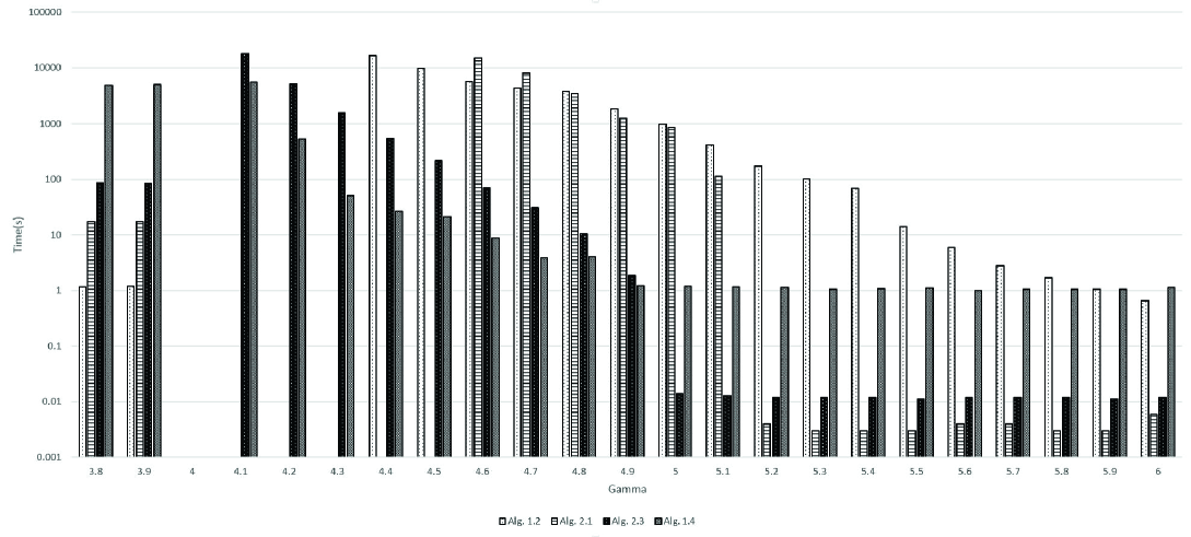
Figure 5: Graph of Table 4: Time(s) vs. $\gamma$ of Algorithms 1.2, 2.1, 2.3 and 21.4 for the graph $G_{12}$.

The symbol “$-$” means that the algorithm did not terminate within 6 hours. The reason for the long computation time may come from the fact that for each graph $G$, the matrix $B_{\gamma}$ lies on the boundary of the copositive cone $\mathcal{COP}_{n}$ when $\gamma=\omega(G)$ ($\omega(G_{8})=3$ and $\omega(G_{12})=4$). See also Figure 5, which shows a graph of the results of Algorithms 1.2, 2.1, 2.3, and 1.4 for the graph $G_{12}$ in Table 4.

We can draw the following implications from the results in Table 4 on page 4 for the larger graph $G_{12}$ (similar implications can be drawn from Table 3):

• At any $\gamma\geq 5.2$, Algorithms 2.1, 1,3, 2.2, 2.3, and 1.4 terminate in one iteration, and the execution times of Algorithms 2.1, 1.3, 2.2, and 2.3 are much shorter than those of Algorithms 1.1, 1.2, or 1.4.

• The lower bound of $\gamma$ for which the algorithm terminates in one iteration and the one for which the algorithm terminates in 6 hours decrease in going from Algorithm 1.3 to Algorithm 3.1. The reason may be that, as shown in Corollary 3.4, the set inclusion relation $\mathcal{G}_{n}\subseteq\mathcal{F}_{n}^{+}\subseteq\mathcal{F}_{n}^{\pm}\subseteq\mathcal{S}_{n}^{+}+\mathcal{N}_{n}$ holds.

• Table 1 on page 1 summarizes the sizes of the LPs for identification. The results here imply that the computational times for solving an LP have the following magnitude relationship for any $n\geq 3$:

  $$\mbox{\bf Algorithm 2.1}<\mbox{\bf Algorithm 1.3}<\mbox{\bf Algorithm 2.2}<\mbox{\bf Algorithm 2.3}.$$

  On the other hand, the set inclusion relation $\mathcal{G}_{n}\subseteq\mathcal{F}_{n}^{+}\subseteq\mathcal{F}_{n}^{\pm}$ and the construction of Algorithms 1 and 2 imply that the detection abilities of the algorithms also follow the relationship described above and that the number of iterations has the reverse relationship for any $\gamma$s in Table 4:

  $$\mbox{\bf Algorithm 2.1}>\mbox{\bf Algorithm 1.3}>\mbox{\bf Algorithm 2.2}>\mbox{\bf Algorithm 2.3}.$$

  It seems that the order of the number of iterations has a stronger influence on the total computational time than the order of the computational times for solving an LP.

• At each $\gamma\in[4.1,4.9]$, the number of iterations of Algorithm 2.3 is much larger than one hundred times those of Algorithm 1.4. This means that the total computational time of Algorithm 2.3 is longer than that of Algorithm 1.3 at each $\gamma\in[4.1,4.9]$, while Algorithm 1.4 solves a semidefinite program of size $O(n^{2})$ at each iteration.

• At each $\gamma<4$, the algorithms show no significant differences in terms of the number of iterations. The reason may be that they all work to find a $v\in V(\{\Delta\})$ such that $v^{T}(\gamma(E-A_{G})-E)v<0$, while their computational time depends on the choice of simplex refinement strategy.

In view of the above observations, we conclude that Algorithm 2.3 with the choices $\mathcal{M}_{n}=\mathcal{F}_{n}^{\pm}$ and $\widehat{\mathcal{M}_{n}}=\widehat{\mathcal{F}_{n}^{\pm}}$ might be a way to check the copositivity of a given matrix $A$ when $A$ is strictly copositive.

The above results are in contrast with those of Bomze and Eichfelder in [10], where the authors show the number of iterations required by their algorithm for testing copositivity of matrices of the form (39). On the contrary to the first observation described above, their algorithm terminates with few iterations when $\gamma<\omega(G)$, i.e., the corresponding matrix is not copositive, and it requires a huge number of iterations otherwise.

It should be noted that Table 3 shows an interesting result concerning the non-convexity of the set $\mathcal{G}_{n}$, while we know that ${\rm conv}\,(\mathcal{G}_{n})=\mathcal{S}_{n}^{+}+\mathcal{N}_{n}$ (see Theorem 2.3). Let us look at the result at $\gamma=4.0$ of Algorithm 2.1. The multiple iterations at $\gamma=4.0$ imply that we could not find $B_{4.0}\in\mathcal{G}_{n}$ at the first iteration for a certain orthogonal matrix $P$ satisfying (6). Recall that the matrix $B_{\gamma}$ is given by (39). It follows from $E-A_{G}\in\mathcal{N}_{n}\subseteq\mathcal{G}_{n}$ and from the result at $\gamma=3.5$ in Table 3 that

$$0.5(E-A_{G})\in\mathcal{G}_{n}\ \mbox{and}\ B_{3,5}=3.5(E-A_{G})-E\in\mathcal{G}_{n}.$$

Thus, the fact that we could not determine whether the matrix

$$B_{4.0}=4.0(E-A_{G})-E=0.5(E-A_{G})+B_{3.5}$$

lies in the set $\mathcal{G}_{n}$ suggests that the set $\mathcal{G}_{n}=\mbox{com}(\mathcal{S}_{n}^{+},\mathcal{N}_{n})$ is not convex.

5.2.2 Results for the matrix arising from standard quadratic optimization problems

In this subsection, we consider the matrix

$$C_{\gamma}:=Q-\gamma E$$ (40)

where $E\in\mathcal{S}_{n}$ is the matrix whose elements are all ones and $Q\in\mathcal{S}_{n}$ is an arbitrary symmetric matrix, not necessarily positive semidefinite. The matrix $C_{\gamma}$ comes from standard quadratic optimization problems of the form,

$$\begin{array}[]{ll}\mbox{Minimize}&x^{T}Qx\\ \mbox{subject to}&x\in\Delta^{S}:=\{x\in\mathbb{R}^{n}_{+}\mid e^{T}x=1\}.\\ \end{array}$$ (41)

In [7], it is shown that the optimal value of the problem

$$p^{*}(Q)=\max\{\gamma\in\mathbb{R}\mid C_{\gamma}\in\mathcal{COP}_{n}\}.$$

is equal to the optimal value of (41).

The instances of the form (41) were generated using the procedure random_qp in [32] with two quartets of parameters $(n,s,k,d)=(10,5,5.0.5)$ and $(n,s,k,d)=(20,10,10.0.5)$, where the parameter $n$ implies the size of $Q$, i.e., $Q$ is an $n\times n$ matrix. It has been shown in [32] that random_qp generates problems, for which we know the optimal value and a global minimizer a priori for each. We set the optimal value as $-10$ for each quartet of parameters.

Tables 5 and 6 show the numerical results for $(n,s,k,d)=(10,5,5,0.5)$ and $(n,s,k,d)=(20,10,10,0.5)$. We generated $2$ instances for each quartet of parameters and performed the seven algorithms on page 5.2 for these instances. Both tables compare the average values of the seven algorithms in terms of the number of iterations (the column “Iter.”) and the total computational time (the column “Time (s)” ): the symbol “$-$” means that the algorithm did not terminate within 30 minutes. In each table, we made the interval between the values $\gamma$ smaller as $\gamma$ got closer to the optimal value, to observe the behavior around the optimal value more precisely.

From the results in Tables 5 and 6 on page 5, we can draw implications that are very similar to those for the maximum clique problem, listed on page 5.2.1 (we hence, omitted discussing them here). A major difference from the implications for the maximum clique problem is that Algorithm 1.2 using the set $\mathcal{H}_{n}$ is efficient for solving a small ($n=10$) standard quadratic problem, while it cannot solve the problem within 30 minutes when $n=20$ and $\gamma\geq-10.3125$.

6 Concluding remarks

In this paper, we investigated the properties of several tractable subcones of $\mathcal{S}_{n}^{+}+\mathcal{N}_{n}$ and summarized the results (as Figures 1 and 2). We also devised new subcones of $\mathcal{S}_{n}^{+}+\mathcal{N}_{n}$ by introducing the semidefinite basis (SD basis) defined as in Definitions 3.2 and 3.3. We conducted numerical experiments using those subcones for identification of given matrices $A\in\mathcal{S}_{n}^{+}+\mathcal{N}_{n}$ and for testing the copositivity of matrices arising from the maximum clique problem and from standard quadratic optimization problems. We have to solve LPs with $O(n^{2})$ variables and $O(n^{2})$ constraints in order to detect whether a given matrix belongs to those cones, and the computational cost is substantial. However, the numerical results shown in Tables 2, 3, 4 and 6 show that the new subcones are promising not only for identification of $A\in\mathcal{S}_{n}^{+}+\mathcal{N}_{n}$ but also for testing copositivity.

Recently, Ahmadi, Dash and Hall [1] developed algorithms for inner approximating the cone of positive semidefinite matrices, wherein they focused on the set $\mathcal{D}_{n}\subseteq\mathcal{S}_{n}^{+}$ of $n\times n$ diagonal dominant matrices. Let $U_{n,k}$ be the set of vectors in $\mathbb{R}^{n}$ that have at most $k$ nonzero components, each equal to $\pm 1$, and define

$$\mathcal{U}_{n,k}:=\{uu^{T}\mid u\in U_{n,k}\}.$$

Then, as the authors indicate, the following theorem has already been proven.

Theorem 6.1 (Theorem 3.1 of [1], Barker and Carlson [3]).

$$\mathcal{D}_{n}=\mbox{\em cone}(\mathcal{U}_{n,k}):=\left\{\sum_{i=1}^{|\mathcal{U}_{n,k}|}\alpha_{i}U_{i}\mid U_{i}\in\mathcal{U}_{n,k},\ \ \alpha_{i}\geq 0\ (i=1,\ldots,|\mathcal{U}_{n,k}|)\right\}$$

From the above theorem, we can see that for the SDP bases $\mathcal{B}_{+}(p_{1},p_{2},\cdots,p_{n})$ in (20), $\mathcal{B}_{-}(p_{1},p_{2},\cdots,p_{n})$ in (22) and $n$-dimensional unit vectors $e_{1},e_{2},\cdots,e_{n}$, the following set inclusion relation holds:

$$\mathcal{B}_{+}(e_{1},e_{2},\cdots,e_{n})\cup\mathcal{B}_{-}(e_{1},e_{2},\cdots,e_{n})\subseteq\mathcal{D}_{n}=\mbox{cone}(\mathcal{U}_{n,k}).$$

These sets should be investigated in the future.

Table 3: Results for $B_{\gamma}$ with $G_{8}$

	Alg. 1.1 $(\mathcal{N}_{n})$		Alg. 1.2 ($\mathcal{H}_{n}$)		Alg. 2.1 ($\mathcal{G}_{n}$ , $\widehat{\mathcal{G}_{n}}$)		Alg. 1.3 ($\mathcal{F}_{n}^{+}$)		Alg. 2.2 ($\mathcal{F}_{n}^{+}$ , $\widehat{\mathcal{F}_{n}^{+}}$)		Alg. 2.3 ($\mathcal{F}_{n}^{\pm}$ , $\widehat{\mathcal{F}_{n}^{\pm}}$)		Alg. 1.4 ($\mathcal{S}_{n}^{+}$ + $\mathcal{N}_{n}$)
$\gamma$	Iter.	Time(s)	Iter.	Time(s)	Iter.	Time(s)	Iter.	Time(s)	Iter.	Time(s)	Iter.	Time(s)	Iter.	Time(s)
1.5	1	0.001	1	0.001	1	0.004	1	0.004	1	0.006	1	0.007	1	0.177
1.6	1	0.001	1	0.001	1	0.004	1	0.004	1	0.006	1	0.008	1	0.139
1.7	1	0.001	1	0.001	1	0.004	1	0.004	1	0.006	1	0.007	1	0.180
1.8	1	0.001	1	0.001	1	0.004	1	0.004	1	0.006	1	0.007	1	0.151
1.9	1	0.001	1	0.001	1	0.004	1	0.004	1	0.006	1	0.007	1	0.225
2.0	159	0.018	159	0.021	159	0.454	159	0.368	159	0.690	159	0.964	159	31.782
2.1	159	0.019	159	0.020	159	0.455	159	0.362	159	0.689	159	0.976	159	31.237
2.2	159	0.019	159	0.020	159	0.454	159	0.363	159	0.698	159	0.971	159	31.352
2.3	159	0.019	159	0.020	159	0.452	159	0.364	159	0.689	159	0.964	159	30.115
2.4	159	0.019	159	0.020	159	0.450	159	0.362	159	0.685	159	0.957	159	30.354
2.5	159	0.019	159	0.020	159	0.453	159	0.364	159	0.690	159	0.964	159	29.681
2.6	159	0.019	159	0.020	159	0.453	159	0.361	159	0.684	159	0.953	159	30.060
2.7	2942	0.495	2422	0.346	2687	7.313	2553	5.623	2461	9.772	2307	12.480	1613	293.441
2.8	2942	0.492	2246	0.301	2463	7.197	1951	4.524	1811	7.355	1635	8.731	1251	448.201
2.9	2942	0.501	1606	0.191	2139	6.270	1493	3.469	1393	5.458	1309	6.867	1251	449.572
3.0	-	-	-	-	-	-	-	-	-	-	-	-	-	-
3.1	263548	261.285	3003	0.279	5885	14.603	1827	3.864	1357	4.879	503	2.394	7	3.186
3.2	255202	243.819	1509	0.132	3129	7.830	911	1.980	377	1.347	201	0.976	3	1.480
3.3	70814	24.332	469	0.040	2229	5.549	447	0.968	249	0.918	111	0.538	3	1.352
3.4	70814	23.735	395	0.034	1603	4.112	291	0.625	167	0.650	53	0.254	3	1.401
3.5	70814	23.821	369	0.031	1	0.003	1	0.003	1	0.004	1	0.004	1	0.322
3.6	70814	24.304	209	0.017	1	0.002	1	0.003	1	0.004	1	0.004	1	0.362
3.7	70814	24.302	115	0.009	1	0.002	1	0.003	1	0.004	1	0.004	1	0.371
3.8	70814	23.744	79	0.007	1	0.002	1	0.003	1	0.004	1	0.004	1	0.359
3.9	70814	24.101	63	0.005	1	0.002	1	0.003	1	0.003	1	0.005	1	0.322
4.0	70814	24.242	47	0.004	227	0.593	1	0.003	1	0.003	1	0.005	1	0.360
4.1	4660	0.431	23	0.002	1	0.003	1	0.003	1	0.003	1	0.005	1	0.324
4.2	4660	0.434	17	0.002	1	0.005	1	0.003	1	0.003	1	0.005	1	0.330
4.3	4660	0.432	17	0.002	1	0.005	1	0.003	1	0.003	1	0.005	1	0.324
4.4	4660	0.433	7	0.001	1	0.005	1	0.003	1	0.003	1	0.005	1	0.328
4.5	4660	0.435	7	0.001	1	0.005	1	0.003	1	0.003	1	0.006	1	0.258

Table 4: Results for $B_{\gamma}$ with $G_{12}$

	Alg. 1.1 $(\mathcal{N}_{n})$		Alg. 1.2 ($\mathcal{H}_{n}$)		Alg. 2.1 ($\mathcal{G}_{n}$ , $\widehat{\mathcal{G}_{n}}$)		Alg. 1.3 ($\mathcal{F}_{n}^{+}$)		Alg. 2.2 ($\mathcal{F}_{n}^{+}$ , $\widehat{\mathcal{F}_{n}^{+}}$)		Alg. 2.3 ($\mathcal{F}_{n}^{\pm}$ , $\widehat{\mathcal{F}_{n}^{\pm}}$)		Alg. 1.4 ($\mathcal{S}_{n}^{+}$ + $\mathcal{N}_{n}$)
$\gamma$	Iter.	Time(s)	Iter.	Time(s)	Iter.	Time(s)	Iter.	Time(s)	Iter.	Time(s)	Iter.	Time(s)	Iter.	Time(s)
2.0	2111	0.483	2111	0.512	2111	8.500	2111	13.782	2111	26.713	2111	49.377	2111	2468.863
2.1	2111	0.483	2111	0.504	2111	8.561	2111	13.682	2111	26.726	2111	49.184	2111	2466.339
2.2	2111	0.482	2111	0.500	2111	8.495	2111	13.585	2111	26.273	2111	48.592	2111	2471.254
2.3	2111	0.483	2111	0.502	2111	8.565	2111	13.520	2111	26.261	2111	48.528	2111	2461.198
2.4	2111	0.489	2111	0.501	2111	8.573	2111	13.315	2111	25.846	2111	47.172	2111	2464.471
2.5	2111	0.485	2111	0.502	2111	8.558	2111	13.344	2111	26.037	2111	47.616	2111	2467.267
2.6	2111	0.481	2111	0.501	2111	8.522	2111	13.304	2111	25.958	2111	47.223	2111	2464.474
2.7	4097	1.136	4097	1.173	4097	16.648	4097	25.753	4097	49.782	4097	90.116	4097	4554.881
2.8	4097	1.136	4097	1.171	4097	16.752	4097	25.655	4097	49.553	4097	89.579	4097	4559.754
2.9	4097	1.134	4097	1.168	4097	16.779	4097	25.643	4097	49.263	4097	89.391	4097	4557.203
3.0	4097	1.134	4097	1.167	4097	16.652	4097	25.550	4097	48.423	4097	87.842	4097	4551.061
3.1	4097	1.136	4097	1.166	4097	16.751	4097	25.484	4097	48.789	4097	87.737	4097	4555.928
3.2	4097	1.138	4097	1.175	4097	16.734	4097	25.422	4097	48.855	4091	87.169	4090	4548.440
3.3	4097	1.131	4095	1.167	4097	16.784	4097	25.274	4091	48.418	4089	86.574	4085	4522.061
3.4	4097	1.131	4087	1.161	4097	16.969	4097	25.179	4091	48.164	4085	86.034	4085	4521.749
3.5	4097	1.139	4085	1.164	4097	16.731	4087	25.122	4087	48.091	4085	85.644	4085	4539.213
3.6	4097	1.137	4085	1.161	4091	16.721	4087	24.920	4087	47.638	4085	84.635	4085	4533.101
3.7	4097	1.140	4085	1.158	4091	16.755	4087	24.834	4085	47.310	4085	84.454	4031	4384.409
3.8	4097	1.133	4084	1.162	4089	17.128	4087	24.831	4085	48.094	4075	85.390	4023	4853.335
3.9	4097	1.137	4080	1.187	4089	17.144	4081	24.719	4079	47.219	4051	84.028	4023	5004.118
4.0	-	-	-	-	-	-	-	-	-	-	-	-	-	-
4.1	-	-	-	-	-	-	-	-	-	-	827717	18054.273	4013	5589.341
4.2	-	-	-	-	-	-	-	-	899627	14932.525	296637	5093.561	345	528.262
4.3	-	-	-	-	-	-	1024493	15985.310	469665	6007.219	102211	1559.054	39	50.717
4.4	-	-	1467851	16744.884	-	-	592539	6657.898	147363	1361.774	36937	545.801	21	26.4293
4.5	-	-	1125035	9820.911	-	-	354083	3066.114	66819	559.987	14533	213.376	17	20.961
4.6	-	-	762931	5680.756	1107483	14991.047	213485	1506.465	25675	206.767	4603	69.503	7	8.768
4.7	-	-	610071	4319.490	793739	8137.410	125747	768.224	22119	180.072	1957	30.490	3	3.809
4.8	-	-	569661	3799.361	473137	3413.271	69887	386.279	20997	176.279	645	10.347	3	4.051
4.9	-	-	407201	1834.912	232295	1231.091	39091	207.440	1969	16.716	109	1.889	1	1.221
5.0	-	-	305627	974.829	190185	859.674	21283	112.276	1213	10.501	1	0.014	1	1.189
5.1	-	-	206949	415.090	34641	113.631	12165	64.742	219	2.000	1	0.013	1	1.150
5.2	-	-	141383	172.541	1	0.004	1	0.008	1	0.008	1	0.012	1	1.120
5.3	-	-	110641	101.475	1	0.003	1	0.008	1	0.007	1	0.012	1	1.040
5.4	-	-	90877	67.681	1	0.003	1	0.008	1	0.008	1	0.012	1	1.078
5.5	-	-	44731	14.292	1	0.003	1	0.007	1	0.007	1	0.011	1	1.100
5.6	-	-	26171	5.910	1	0.004	1	0.007	1	0.007	1	0.012	1	1.000
5.7	-	-	15045	2.775	1	0.004	1	0.008	1	0.008	1	0.012	1	1.057
5.8	-	-	10239	1.705	1	0.003	1	0.007	1	0.007	1	0.012	1	1.063
5.9	-	-	6977	1.042	1	0.003	1	0.007	1	0.007	1	0.011	1	1.051
6.0	-	-	4717	0.654	1	0.006	1	0.007	1	0.008	1	0.012	1	1.119

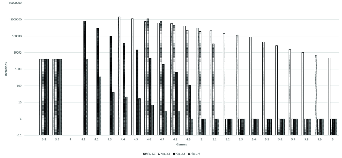
Figure 4: Graph of Table 4: Iterations vs. $\gamma$ of Algorithms 1.2, 2.1, 2.3 and 21.4 for the graph $G_{12}$.

Table 5: Results for $C_{\gamma}$ with $n=10$

	Alg. 1.1 $(\mathcal{N}_{n})$		Alg. 1.2 ($\mathcal{H}_{n}$)		Alg. 2.1 ($\mathcal{G}_{n}$ , $\widehat{\mathcal{G}_{n}}$)		Alg. 1.3 ($\mathcal{F}_{n}^{+}$)		Alg. 2.2 ($\mathcal{F}_{n}^{+}$ , $\widehat{\mathcal{F}_{n}^{+}}$)		Alg. 2.3 ($\mathcal{F}_{n}^{\pm}$ , $\widehat{\mathcal{F}_{n}^{\pm}}$)		Alg. 1.4 ($\mathcal{S}_{n}^{+}$ + $\mathcal{N}_{n}$)
$\gamma$	Iter.	Time(s)	Iter.	Time(s)	Iter.	Time(s)	Iter.	Time(s)	Iter.	Time(s)	Iter.	Time(s)	Iter.	Time(s)
-5.00000	1	0.001	1	0.001	1	0.009	1	0.009	1	0.016	1	0.025	1	0.501
-7.50000	1	0.001	1	0.001	1	0.010	1	0.009	1	0.016	1	0.025	1	0.491
-8.75000	1	0.001	1	0.001	1	0.010	1	0.008	1	0.016	1	0.025	1	0.481
-9.37500	2	.001	2	0.001	2	0.020	2	0.018	2	0.032	2	0.048	2	0.946
-9.68750	3	0.001	3	0.001	3	0.021	3	0.021	3	0.041	3	0.066	3	1.621
-9.84375	799	0.267	799	0.259	799	4.993	799	4.815	799	9.253	799	15.329	799	441.790
-10.00000	-	-	-	-	-	-	-	-	-	-	-	-	-	-
-10.15625	84828	81.527	1	0.001	1	0.029	1	0.007	1	0.011	1	0.012	1	0.424
-10.31250	39790	17.030	1	0.001	1	0.004	1	0.008	1	0.011	1	0.012	1	0.362
-10.62500	5546	1.210	1	0.001	1	0.005	1	0.008	1	0.011	1	0.012	1	0.380
-11.25000	8	0.007	1	0.001	1	0.005	1	0.007	1	0.011	1	0.012	1	0.363
-12.50000	2	0.001	1	0.001	1	0.005	1	0.007	1	0.011	1	0.012	1	0.367
-15.00000	2	0.001	1	0.001	1	0.005	1	0.008	1	0.011	1	0.012	1	0.384

Table 6: Results for $C_{\gamma}$ with $n=20$

	Alg. 1.1 $(\mathcal{N}_{n})$		Alg. 1.2 ($\mathcal{H}_{n}$)		Alg. 2.1 ($\mathcal{G}_{n}$ , $\widehat{\mathcal{G}_{n}}$)		Alg. 1.3 ($\mathcal{F}_{n}^{+}$)		Alg. 2.2 ($\mathcal{F}_{n}^{+}$ , $\widehat{\mathcal{F}_{n}^{+}}$)		Alg. 2.3 ($\mathcal{F}_{n}^{\pm}$ , $\widehat{\mathcal{F}_{n}^{\pm}}$)		Alg. 1.4 ($\mathcal{S}_{n}^{+}$ + $\mathcal{N}_{n}$)
$\gamma$	Iter.	Time(s)	Iter.	Time(s)	Iter.	Time(s)	Iter.	Time(s)	Iter.	Time(s)	Iter.	Time(s)	Iter.	Time(s)
-5.00000	1	0.002	1	0.002	1	0.042	1	0.095	1	0.181	1	0.182	1	13.812
-7.50000	1	0.002	1	0.002	1	0.045	1	0.093	1	0.183	1	0.180	1	14.266
-8.75000	2	0.005	2	0.005	2	0.046	2	0.191	2	0.368	2	0.378	2	25.224
-9.37500	128	0.091	128	0.096	128	2.490	128	11.755	128	22.660	128	22.682	128	1598.031
-9.68750	-	-	-	-	-	-	-	-	-	-	-	-	-	-
-9.84375	-	-	-	-	-	-	-	-	-	-	-	-	-	-
-10.00000	-	-	-	-	-	-	-	-	-	-	-	-	-	-
-10.15625	-	-	-	-	-	-	1	0.080	1	0.080	1	0.076	1	13.912
-10.31250	-	-	-	-	1	0.010	1	0.072	1	0.072	1	0.073	1	14.015
-10.62500	-	-	2	0.001	1	0.009	1	0.072	1	0.069	1	0.073	1	14.135
-11.25000	-	-	2	0.001	1	0.009	1	0.067	1	0.067	1	0.071	1	12.126
-12.50000	3187	1.370	2	0.001	1	0.010	1	0.068	1	0.066	1	0.067	1	11.128
-15.00000	2	0.001	2	0.001	1	0.010	1	0.069	1	0.080	1	0.068	1	9.580

References

- [1] Ahmadi, A. A., Dash, S., & Hall, G. (2015). Optimization over structured subsets of positive semidefinite matrices via column generation, arXiv:1512.05402 [math.OC].
- [2] Alizadeh, F. (2012). An Introduction to formally real Jordan algebras and their applications in optimization, Handbook on Semidefinite, Conic and Polynomial Optimization (pp. 297-337). Springer US.
- [3] Barker, G. P., & Carlson, D. (1975). Cones of diagonally dominant matrices. Pacific Journal of Mathematics, 57, 15-32.
- [4] Berman, A. (1973). Cones, Matrices and Mathematical Programming, Lecture Notes in Economics and Mathematical Systems 79, Springer-Verlag.
- [5] Berman, A., & Monderer, N. S. (2003). Completely Positive Matrices, World Scientific Publishing.
- [6] Bomze, I. M. (1996). Block pivoting and shortcut strategies for detecting copositivity. Linear Algebra and its Applications, 248(15), 161-184.
- [7] Bomze, I. M., Dür, M., De Klerk, E., Roos, C., A. J. Quist, A. J., & Terlaky, T. (2000). On copositive programming and standard quadratic optimization problems. Journal of Global Optimization, 18(4), 301-320.
- [8] Bomze, I. M., & De Klerk, E. (2002). Solving standard quadratic optimization problems via linear, semidefinite and copositive programming. Journal of Global Optimization, 24(2), 163-185.
- [9] Bomze, I. M. (2012). Copositive optimization - recent developments and applications. European Journal of Operational Research, 216(3), 509-520.
- [10] Bomze, I. M., & Eichfelder, G. (2013). Copositivity detection by difference-of-convex decomposition and -subdivision. Mathematical Programming, Series A, 138(1), 365-400.
- [11] Brás, C., Eichfelder, G., & Júdice, J. (2015). Copositivity tests based on the linear complementarity problem. Computational Optimization and Applications, 1-33.
- [12] Bundfuss, S., & Dür, M. (2008). Algorithmic copositivity detection by simplicial partition. Linear Algebra and its Applications, 428(7), 1511-1523.
-
[13]
Bundfuss, S. (2009).
Copositive matrices, copositive programming, and applications.
Ph.D. Dissertation, TU Darmstadt.
Available online athttp://www3.mathematik.tu-darmstadt.de/index.php?id=483(confirmed on March 20, 2017). - [14] Burer, S. (2009) On the copositive representation of binary and continuous nonconvex quadratic programs. Mathematical Programming, 120(4), 479-495.
- [15] De Klerk, E., & Pasechnik, D. V. (2002). Approximation of the stability number of a graph via copositive programming. SIAM Journal on Optimization, 12, 875-892.
- [16] Deng, Z., Fang, S.-C., Jin, Q., & Xing, W. (2013). Detecting copositivity of a symmetric matrix by an adaptive ellipsoid-based approximation scheme. European Journal of Operations research, 229(1), 21-28.
- [17] Diananda, P. H. (1962). On non-negative forms in real variables some or all of which are non-negative. Mathematical Proceedings of the Cambridge Philosophical Society, 58(1), 17-25.
- [18] Dickinson, P. J. C. (2011). Geometry of the copositive and completely positive cones. Journal of Mathematical Analysis and Applications, 380, 377-395.
- [19] Dickinson, P. J. C. (2014). On the exhaustivity of simplicial partitioning. Journal of Global Optimization, 58(1), 189-203.
- [20] Dickinson, P. J. C., & Gijben, L. (2014). On the computational complexity of membership problems for the completely positive cone and its dual. Computational Optimization and Applications, 57(2), 403-415.
- [21] Dür, M. (2010). Copositive programming - a survey, Recent Advances in Optimization and Its Applications in Engineering (pp.3-20). Springer-Verlag.
- [22] Dür, M., & Hiriart-Urruty, J.-B. (2013). Testing copositivity with the help of difference-of-convex optimization. Mathematical Programming, 140(1), 31-43.
- [23] Faraut, J., & Korányi, A. (1994). Analysis on Symmetric Cones, Oxford University Press.
- [24] Fenchel, W. (1953). Convex cones, sets and functions, mimeographed notes by D. W. Blackett, Princeton Univ. Press, Princeton, N. J.
- [25] Fiedler, M., & Pták, V. (1962). On matrices with non-positive off-diagonal elements and positive principal minors. Czechoslovak Mathematical Journal, 12(3), 382-400.
- [26] Golub, G. H., & Van Loan, C. F. (1996). Matrix Computations, Johns Hopkins University Press; Third edition.
- [27] Horst, R. (1997). On generalized bisection of -simplices. Mathematics of Computation, 66(218), 691-698.
- [28] Horn, R. A., & Johnson, C. R. (1985). Matrix Analysis, Cambridge University Press.
- [29] Jarre, F., & Schmallowsky, K. (2009). On the computation of certificates. Journal of Global Optimization, 45(2), 281-296.
- [30] Johnson, C. R., & Reams, R. (2008). Constructing copositive matrices from interior matrices. The Electronic Journal of Linear Algebra 17(1), 9-20.
- [31] Murty, K. G., & Kabadi, S. N. (1987). Some NP-complete problems in quadratic and nonlinear programming. Mathematical Programming, 39(2), 117-129.
-
[32]
Nowak, I. (1998)
A global optimality criterion for nonconvex quadratic programming over a simplex.
Pre-Print 98–17, Humboldt University, Berlin. Available online at
http://wwwiam. mathematik.hu-berlin.de/ivo/ivopages/work.html(confirmed on March 20, 2017). - [33] Povh, J., & Rendl, F. (2007). A copositive programming approach to graph partitioning. SIAM Journal on Optimization, 18(1), 223-241.
- [34] Povh, J., & Rendl, F. (2009). Copositive and semidefinite relaxations of the quadratic assignment problem. Discrete Optimization, 6(3), 231-241.
- [35] Rockafellar, R. T., & Wets, R. J-B. (1998). Variational Analysis. Springer.
- [36] Sponsel, J., Bundfuss, S., & Dür, M. (2012). An improved algorithm to test copositivity. Journal of Global Optimization, 52(3), 537-551.
- [37] Tanaka, A., & Yoshise, A. (2015). An LP-based algorithm to test copositivity. Pacific Journal of Optimization, 11(1), 101-120.
- [38] Yoshise, A., & Matsukawa, Y. (2010). On optimization over the doubly nonnegative cone. Proceedings of 2010 IEEE Multi-conference on Systems and Control, 13-19.
- [39] Z̆ilinskas, J., & Dür, M. (2011). Depth-first simplicial partition for copositivity detection, with an application to MaxClique. Optimization Methods and Software 26(3), 499-510.